Hybrid Method for Detecting Anomalies in Cosmic ray Variations Using Neural Networks Autoencoder

Abstract

Cosmic rays were discovered by the Austrian physicist Victor Hess in 1912 in a series of balloon experiments performed between 1911 and 1912. Cosmic rays are an integral part of fundamental and applied research in the field of solar–terrestrial physics and space weather. Cosmic ray data are applied in different fields from the discovery of high-energy particles coming to Earth from space, and new fundamental symmetries in the laws of nature, to the knowledge of residual matter and magnetic fields in interstellar space. The properties of interplanetary space are determined from intensity variations, angular distribution, and other characteristics of galactic cosmic rays. The measure of cosmic ray flux intensity variability is used as one of the significant space weather factors. The negative impact of cosmic rays is also known. The negative impact can significantly increase the level of radiation hazard and pose a threat to astronauts, crews, and passengers of high-altitude aircraft on polar routes and to modern space equipment. Therefore, methods aimed at timely detection and identification of anomalous manifestations in cosmic rays are of particular practical relevance. The article proposes a method for analyzing cosmic ray variations and detecting anomalous changes in the rate of galactic cosmic ray arrival to the Earth. The method is based on a combination of the Autoencoder neural network with wavelet transform. The use of non-linear activation functions and the ability to flexibly change the structure of the network provide the ability of the Autoencoder to approximate complex dependencies in the recorded variations of cosmic rays. The article describes the numerical operations of the method implementation. Verification of the adequacy of the neural network model is based on the use of Box–Ljung Q-statistics. On the basis of the wavelet transform constructions, data-adaptive operations for detecting complex singular structures are constructed. The parameters of the applied threshold functions are estimated with a given confidence probability based on the $\alpha$-quantiles of Student’s distribution. Using data from high-latitude neutron monitor stations, it is shown that the proposed method provides efficient detection of anomalies in cosmic rays during increased solar activity and magnetic storms. Using the example of a moderate magnetic storm on 10–11 May 2019, the necessity of applying different methods and approaches to the study of cosmic ray variations is confirmed, and the importance of taking them into account when making space weather forecast is shown.

1. Introduction

Cosmic rays are a mysterious and interesting natural phenomenon. They were first discovered in the second decade of the 20th century by virtue of the experiments of great scientists such as Victor Hess, Werner Kolcherster, and others [1,2]. Currently, using modern equipment, scientists are actively investigating the intensity of the cosmic ray flux, the composition of cosmic particles, and their energy spectrum and angular distribution [3,4,5,6,7]. Cosmic rays (CR) are of exceptional interest in solving urgent problems in the field of astrophysics [8,9,10,11,12], nuclear physics, and many other applied areas (research of rocks, moisture content, mastering high altitudes by aviation, etc.) [13,14,15]. In the field of astrophysics, X-rays, γ-radiation, and cosmic radio emission are most often generated by electrons, protons, and CR nuclei. The properties of interplanetary space are determined from intensity variations, angular distribution, and other characteristics of CR. The negative impact of anomalous galactic cosmic ray flows is also known. They significantly increase the level of radiation hazard for astronauts, crews, and passengers of high-altitude aircrafts on polar routes. Negative impacts can lead to loss of satellites and failure of space equipment [16,17,18,19]. A special class of proton events are the so-called strong ground level enhancement (GLE). Using GLE data, the maximum energy of cosmic ray protons is fixed. Especially dangerous is the combination of the beginning of a magnetic storm with the arrival of CR to the Earth from a powerful proton event on the Sun. Examples of such events are 6–7 April and 15–16 July 2000 [20]. GLE 72 (10 September 2017) was particularly strong and was measured for the first time on more than one planet (Mars and Earth), and it is of particular interest during the solar minimum [21]. Then, during magnetic storms, powerful solar cosmic ray fluxes penetrated into the Earth’s magnetosphere and atmosphere up to middle latitudes. It is fluorescence light coming from the excitation of the nitrogen and oxygen molecules of the Earth’s atmosphere (thermosphere/exosphere) caused by the energetic particles trapped in the Van Allen’s belts (protons and electrons) that during more turbulent periods can interact with these atmospheric layers at high latitudes [21].

Anomalous phenomena and processes on the Sun are reflected in the recorded CR intensity variations. Therefore, CR is one of the significant factors in space weather. Fast changes in the outer part of the radiation belts during solar events indicate the presence of high-speed mechanisms for replenishing the outer belt with electrons [18]. In the works of various authors [22,23,24,25,26,27,28], anomalous changes in the CR flux preceding the onset of magnetic storms are noted. The observed Forbush effects can be characterized by both an unexpected anomalous increase and an anomalous decrease in galactic cosmic ray intensity. The importance of taking into account CR in space weather is confirmed by the correlation of galactic cosmic ray variability with Dst geomagnetic index obtained by the authors [24], which has a maximum with a delay of several hours. In turn, the results of [29] suggest that all CME properties have some correlation with CRI, but the definition of the most significant parameter is still open.

The abovementioned information indicates the need to develop methods for the CR analysis. Among these, methods aimed at diagnosing abnormal manifestations in CR are of particular practical relevance [22,23,24,30,31]. One of the most successful methods in this area is the “Ring of Station Method”, developed by a group of scientists [4]. This method is based on the calculation of the hourly longitudinal distribution of the count rate of particles recorded by a network of ground stations of neutron monitors (NM) [32]. Data from neutron monitors are secondary cosmic rays recorded by ground-based detectors. They reflect the intensity of cosmic radiation and are an important source of space weather. The Ring of Station Method works best when using data from high-latitude neutron monitors, but with the exception of near-polar stations [4]. However, the conditions for implementing this method are not always fulfilled due to the uneven distribution of stations around the globe and the significant impact of natural and technogenic noise on measurement results. In addition, it is difficult to quantify the results of the method and, as a consequence, to evaluate their accuracy and quality.

Traditional averaging methods [33] are aimed at studying regular variations in CR. However, they are ineffective for detecting anomalous changes that occur during extreme solar events and magnetic storms. A significant disadvantage of these methods is also the risk of information distortion and, as a result, either the occurrence of a “false” alarm signal or the loss of an anomaly.

To analyze the CR, machine learning methods are being actively developed [34,35,36,37]. For example, the author of [36] proposed the use of graph neural networks to study the CR energy spectrum and composition. This approach reduces time and computational costs, and also provides more accurate results compared to the traditional method based on the likelihood function. At present, the analysis of data by this method is limited due to the specific configuration of the detector used, but the authors of [37] are actively conducting the research and plan to expand the capabilities of the method up to the study of the primary energies of cosmic rays.

To study natural data, the wavelet transform [38,39] and hybrid methods built on them [24,25,30,40,41,42,43] are widely used. For example, the study by [41] proposed the use of the wavelet transform to analyze CR variations and to predict magnetic storms. The authors of [41], on the basis of the use of Morlet wavelets [41], managed to identify a 24-h periodicity in CR variations during quiet time. At the times of strong magnetic storms, this periodicity is violated, and there is another, well-defined 12-h fluctuation [41]. The limitations of this method include the fact that its effectiveness has been confirmed only for strong magnetic storms, and data from only one station were used in the studies. The authors of [30] compared the wavelet transform with the Fourier method to research CR variations. The results of [30] confirmed the efficiency of the wavelet transform for the analysis of CR time evolution.

Flexible constructions of the wavelet transform and a wide set of bases [43] make it possible to construct data-adaptive processing and analysis operations and to detect complex singular structures. This allows one to develop complex hybrid approaches to the analysis of complex data using the wavelet transform. For example, in the paper [24], the F-filter was applied together with wavelet transform to detect low-amplitude periodicities [44]. The F-filter makes it possible to evaluate the variability of the process within the analyzed time interval and to detect more clearly the “hidden” patterns in the data. The authors of this article propose a method for detecting anomalous changes in the CR arrival rate to the Earth. It is close to the [24] approach and is based on a combination of wavelet transform constructions with adaptive thresholds [26]. The results of [26] confirmed the high efficiency of the combination of different methods for CR data analysis. Using the data from neutron monitors at high-latitude stations, the work of [26] shows the effectiveness of the method for detecting small anomalies in CR that precede magnetic storms of various nature and strength. The results of [26] are important. They confirm the correlation of the CR variability with Dst index, with a maximum having a time delay [24], making it possible to predict the beginning of the magnetic storm development. The revealed anomalies in CR [26] reached the highest intensity 2–6 h before the onset of magnetic storms. This work continues this research.

The method of [26] has shown good results for detecting multiscale anomalies in CR. The high detecting ability of wavelets and their combination with adaptive thresholds provide efficient detection of multiscale short-period anomalies of different intensity and duration. The anomaly detection rate was over 86%, with a false alarm rate of 9% [26]. However, for the detection of narrow spectrum anomalies, as it was shown earlier in [45], the Autoencoder neural network [46,47], followed by the construction of wavelet spectra, is more efficient. The Autoencoder provides the identification of hidden non-linear dependencies, has high adaptive ability, and is able to significantly reduce the noise level [46]. The use of nonlinear activation functions in the hidden layer of the network, as well as the ability to increase the number of hidden layers, provides the ability of the Autoencoder to approximate data of complex nonlinear structure. In this paper, we propose a method based on a combination of the Autoencoder network with a wavelet transform. The numerical operations of the method implementation are constructed. Verification of the adequacy of the neural network model is based on the use of $Q$-statistics of Box–Ljung [48]. To detect anomalies in the wavelet space, the use of threshold functions is proposed, the parameters of which are estimated on the basis of the $\alpha$-quantiles of Student’s distribution. Using data from high-latitude neutron monitor stations as an example, it is shown that the proposed combination of the Autoencoder with wavelet transform allows one to adapt to the changing structure of CR variations and provides detection of anomalies of different time-frequency structures.

2. Materials and Methods

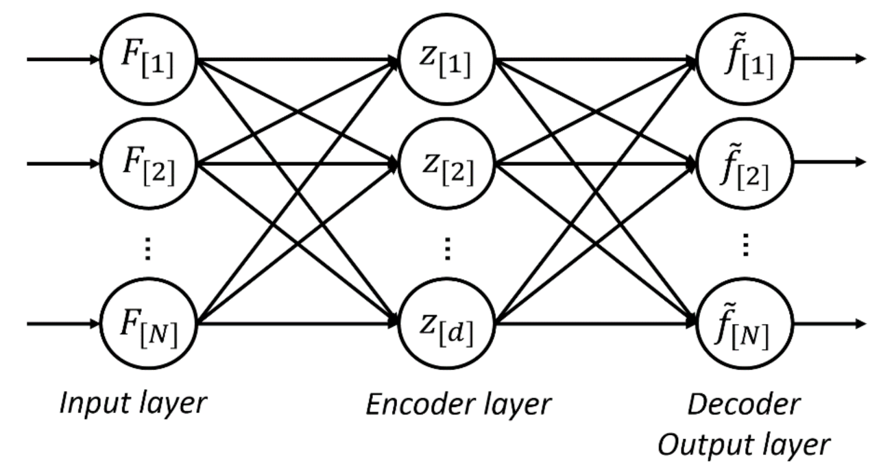
2.1. Approximation of Data on the Basis of the Autoencoder Neural Network

Let us have a discrete time series $F\left[n\right]$ ($nϵ\mathbb{N}$, $\mathbb{N}$ are natural numbers):

$$F\left[n\right]=f\left[n\right]+e\left[n\right],$$

(1)

where $F\left[n\right]$ are observed data; $f\left[n\right]$ are true values hidden in noise; and $e\left[n\right]$ is noise.

The values $f\left[n\right]$ are considered as elements of a special set $\theta$, not taking into account the probability distribution on it [49]. Then, according to the Minimax Criteria [49], the task of estimating $f$ is to determine such a solution operator $D$, that minimizes the risk

$$r_O\left(\theta \right)=in{f}_{DϵO}su{p}_{fϵ\theta }E\left\{{\Vert \tilde{f}-f\Vert }^2\right\},$$

where $E$ is the expectation, ${\Vert ·\Vert }^2$ is the Euclidean norm or $l^2$-norm, $O$ is the operators set, $\widetilde{f }$ is the estimate of $f$.

Let us consider the nonlinear mapping, performed by the Autoencoder neural network, as a decision operator $D$, a nonlinear mapping, performed by the Autoencoder neural network [46,47]. The typical architecture of the Autocorder network is shown in Figure 1.

The presented architecture has three layers, namely, input, hidden (encoder), and output (decoder) [46]. The dimension of the output of the neural network is equal to the dimension of the input. The encoder maps the input vector F to the vector $z$:

$$z=h^{\left(1\right)}\left(V^{\left(1\right)}F+b^{\left(1\right)}\right),$$

(2)

where the superscript (1) is the layer number, $h^{\left(1\right)}\in {ℝ}^{d\times 1}$ is the nonlinear activation function, $V^{\left(1\right)}\in {ℝ}^{d\times N}$ is the weight matrix, $F\in {ℝ}^{N\times 1}$ is the input vector, $N$ is the dimension of the input vector, $b^{\left(1\right)}\in {ℝ}^{d\times 1}$ is the displacement vector, and $ℝ$ are real numbers.

The decoder maps the encoded representation of $z$ back, the obtained estimate

$$\tilde{f}=h^{\left(2\right)}\left(V^{\left(2\right)}z+b^{\left(2\right)}\right),$$

(3)

where the superscript (2) is the layer number, $h^{\left(2\right)}\in {ℝ}^{N\times 1}$ is the linear activation function, $V^{\left(2\right)}\in {ℝ}^{N\times d}$ is the weight matrix, and $b^{\left(2\right)}\in {ℝ}^{N\times 1}$ is the displacement vector.

Thus, from (2) and (3) based on the network, we obtain the estimate

$$\tilde{f}=h^{\left(2\right)}\left(V^{\left(2\right)}\left(h^{\left(1\right)}\left(V^{\left(1\right)}F+b^{\left(1\right)}\right)\right)+b^{\left(2\right)}\right).$$

(4)

The risk of estimating $\tilde{f}$ is

$$r\left(D,f\right)=E\left\{{\Vert \tilde{f}-f\Vert }^2\right\}.$$

Assuming that the noise $e\left[n\right]$ is uncorrelated (see (1)), following the work of [47], we take $d<N$ ($d$ is the dimension of the hidden layer of the network, see Figure 1), and we build the optimization procedure for the estimate $\tilde{f}$ on cost function minimization

$$C={\displaystyle \sum }_{k=1}^M\Vert {\tilde{f}}^{\left(k\right)}-F^{\left(k\right)}\Vert {}^2\to mi{n}_{\aleph }$$

where $\aleph =\left\{V^{\left(1\right)}, V^{\left(2\right)},b^{\left(1\right)},b^{\left(2\right)}\right\}$, and $M$ is the number of examples on which the neural network is trained.

The dimension of the hidden layer ($d<N$) is smaller than the input data and it provides the selection of significant dependencies when training the network. Noise is suppressed due to data compression [47]. The dependencies, identified by the network, define the data feature space. The overlap of this space, in the case of constructing an adequate neural network model, allows one to restore the original data with acceptable accuracy at the decoding stage.

Taking into account the assumption of uncorrelated noise, to check the adequacy of the obtained model, Box–Ljung $Q$-statistics can be applied to its residual errors [48]. The Box–Ljung statistic tests the hypothesis that all autocorrelations ${\rho }_i$ of the time series up to order m inclusive are equal to zero, i.e., hypothesis $H_0$: ${\rho }_1={\rho }_2=\dots ={\rho }_m$ versus alternative hypothesis $H_1$: ${\displaystyle \sum }_{i=1}^m{\rho }_i^2>0$.

$Q$-statistics has an asymptotic distribution ${\chi }_m^2$ and is calculated by the following formula [35]:

$$Q=\left(T+2\right)T{\displaystyle \sum }_{i=1}^m{\left(T-i\right)}^{-1}{r}_i^2,$$

(5)

where $T$ is the number of observations, and $r_i$ is the estimate of ${\rho }_i$ from sampled data.

If the null hypothesis $H_0$, is confirmed, then the resulting neural network model can be taken as adequate. Then, the estimated $\tilde{f}$ (see (4)) contains significant data features and a low noise level with a high probability.

2.2. Detection of Anomalies in Data on the Basis of the Wavelet Transform

On the basis of the continuous wavelet transform, the mapping $\tilde{f}\in L^2\left(ℝ\right)$ ($L^2\left(ℝ\right)$ is the Lebesgue space [38,39]) into the wavelet space can be performed:

$$W\tilde{f}\left(s,u\right)={{\displaystyle \int }}_{-\infty }^{+\infty }\tilde{f}\left(t\right)\frac{1}{\sqrt{s}}{\Psi }^{\ast }\left(\frac{t-u}{s}\right)dt,$$

(6)

where $\Psi$ is a wavelet; $s$ is a scale; $u$ is a time shift; $s,u \in ℝ$; and $s\ne 0$.

Since the amplitude of the coefficients $\left|W\tilde{f}\left(s,u\right)\right|$ characterizes the amplitude of the local singularity of the function $\tilde{f}$ on the scale $s$ in the vicinity of the point $t=u$ [38,39], an increase in the amplitude indicates the occurrence of an anomaly in the vicinity of this point. In this case, thresholds $T_s$ can be applied to detect anomalies at the scale s:

$$P_{T_s}\left[W\tilde{f}\left(s,u\right)\right]=\left\{\begin{array}{c}W\tilde{f}\left(s,u\right), if\left|W\tilde{f}\left(s,u\right)\right|\ge T_s,\\ 0, if\left|W\tilde{f}\left(s,u\right)\right|<T_s.\end{array}\right.$$

(7)

Outside the locality containing local (anomalous) features, the values $W\tilde{f}\left(s,u\right)$ are close to zero in $u$ [43]. Taking into account that the anomalous feature is a rare event, there is a high probability ($\alpha \approx 0,99$) that the values $\left|W\tilde{f}\left(s,u\right)\right|$ by the argument $u$ are in the interval $\left(\mu -3\sigma ; \mu +3\sigma \right)$, where $\mu \approx 0$ is the expectation of the value $\left|W\tilde{f}\left(s,u\right)\right|$, $\sigma$ is the standard deviation (three-sigma rule [50]), and the value $\left|W\tilde{f}\left(s,u\right)\right|$ has an asymptotically normal distribution.

In the case of normality $\left|W\tilde{f}\left(s,u\right)\right|$, we can estimate the thresholds $T_s$ with a given confidence probability $\alpha$, estimating the thresholds as

$$T_s=t_{1-\frac{\alpha }{2},N-1}{\widehat{\sigma }}_s,$$

where $t_{\alpha ,N}$ are the $\alpha$-quantiles of Student’s distribution [50], and ${\widehat{ \sigma }}_s$ is the sample standard deviation. For example, for a confidence level $\alpha =0.95$, we set $T_s=t_{0.5,1439}{\widehat{\sigma }}_s=1.96{\widehat{\sigma }}_s$.

Taking into account the non-stationarity of the process, following the work [26], we estimate the thresholds in a sliding time window. In this case, we take

$$T_s^l=t_{1-\frac{\alpha }{2},L-1}{\widehat{\sigma }}_s^l,$$

(8)

where ${\widehat{\sigma }}_s^l=\sqrt{\frac{1}{L-1}{{\displaystyle \sum }}_{m=1}^L{(W\tilde{f}\left(s,u\right)-\overline{W\tilde{f}\left(s,u\right)})}^2}.L$ is the time window length.

For the identified anomalies, their intensity at time $t=u$ can be estimated as [26]

$$E_u={\displaystyle \sum }_s{P}_{T_s^l}\left[W\tilde{f}\left(s,u\right)\right].$$

(9)

which will be positive in case of an anomalous increase in the function values (positive anomaly) and negative in the case of an anomalous decrease in the function values (negative anomaly).

Relations (6)–(9) are defined in the space of continuous functions $L^2\left(ℝ\right)$. It follows from the equivalence of the continuous and discrete wavelet transform that for discrete data $\tilde{f}\left[n\right]$, performing execution of operation (6) is equivalent to representing them as a series [38,39]:

$$\tilde{f}\left[n\right]={\displaystyle \sum }_{j,k=-\infty }^{\infty }{c}_{jk}{\Psi }_{jk}\left[n\right],$$

(10)

where ${\Psi }_{jk}=2^{\frac{j}{2}}\Psi \left(2^{j}n-k\right), j,k\in N, c_{jk}=\tilde{f},{\Psi }_{jk}$ are the coefficients of the expansion of the function $\tilde{f}$ into a series in terms of orthogonal wavelets.

The expansion coefficients in series (10) are defined as $c_{jk}=W\tilde{f}\left(\frac{1}{2^j},\frac{k}{2^j}\right)$ [38,39]. Correspondingly, taking into account (8), mapping (7) will take the form:

$$P_{T_j^l}\left[W\tilde{f}\left(\frac{1}{2^j},\frac{k}{2^j}\right)\right]=\left\{\begin{array}{c}W\tilde{f}\left(\frac{1}{2^j},\frac{k}{2^j}\right), if\left|W\tilde{f}\left(\frac{1}{2^j},\frac{k}{2^j}\right)\right|\ge T_j^l,\\ 0, if\left|W\tilde{f}\left(\frac{1}{2^j},\frac{k}{2^j}\right)\right|<T_j^l.\end{array}\right.$$

(11)

To estimate the intensity of anomalies, in accordance with (9), we obtain

$$E_k={\displaystyle \sum }_j{P}_{T_j^l}\left[W\tilde{f}\left(\frac{1}{2^j},\frac{k}{2^j}\right)\right].$$

(12)

3. Results

Due to the anisotropy properties, cosmic ray variations recorded at different stations may have different characteristics [51,52]. Therefore, as it was noted in [51], in order to detect anomalous changes in the CR, it is important to perform analysis on the basis of the station network data. High-latitude stations, not circumpolar ones, are the most proper for the analysis of CR dynamics [51,52]. Due to the narrowness of the longitudinal receiving zone, they have the highest sensitivity to the longitudinal anisotropy of cosmic rays. This is expressed in the largest acceptance coefficients for the equatorial component of cosmic ray vector anisotropy [51].

The data of high-latitude station network of neutron resource monitors [53] were used in the work. Below are the results of data processing from Inuvik (INVK, Coord: 68.36, −133.72), Oulu (OULU, Coord: 65.0544, 25.4681), and Thule (THUL, Coord: 76.5, −68.7) stations. The choice of these stations was determined by the presence of representative statistics to ensure the training procedure for neural networks, as well as the absence of gaps in the data during the analyzed periods.

The data of each station are taken as a separate dataset. Accordingly, neural networks (NN) were trained separately for each station. The architecture of NN for each station was the same. The NN parameters for each station were determined separately at the training stage. Taking into account the CR anisotropy properties, data analysis was performed separately for different levels of solar activity. The NN were implemented in the MATLAB application package [54], and the Deep Learning Toolbox framework was used. NN was trained on the basis of the error back propagation method, taking into account the use of the sparsity regularizer [54]. When constructing NN training sets, data were selected on the basis of the analysis of space weather factors. We used data that were recorded during the periods of absence of Forbush effects in the CR, disturbances in the magnetosphere, and low flare activity. The length of the training sample for each NN was at least 100 days. No training datasets were used in the analysis.

Following the results of the work [45], the NN input vector dimension was 1440 samples that corresponded to a day (minute data). The NN hidden layer dimension was determined empirically. The smallest errors on the training and test sets were obtained for the dimension of the layer $d=\frac{N}{2}$.

The Q-criterion was used to check the adequacy of the constructed NNs. Estimates by the Q-criterion (see (5)) showed that $Q_{stat}<Q_{crit}=31.4$ under the alternative hypothesis for the significance level $=0.05$. In particular, for station Oulu, $Q_{stat}=23.12$; for station Inuvik, $Q_{stat}=22.89$; for station Thule, $Q_{stat}=27.03$. Therefore, the hypothesis about the joint equality to zero of all autocorrelations of the time series up to the order m inclusive is not rejected and the adequacy of the constructed NNs is confirmed.

To test the normality of $\left|W\tilde{f}\left(s,u\right)\right|$ for the argument $u,$ Pearson’s criterion was used [50]. As an example, Figure 2 shows the histograms of wavelet coefficients $\left|W\tilde{f}\left(500,u\right)\right|$ and $\left|W\tilde{f}\left(1000,u\right)\right|$. Operations (9)–(11) were performed using Coiflet 2 wavelets [39,43]. In operation (10), thresholds $T_s=1.96{\widehat{\sigma }}_s^l$, were used for I = 1440.

Figure 3 shows the results of the method during weak magnetic storms at high latitudes. The neutron monitor data of the Oulu station (Coord: 65.0544, 25.4681) were analyzed. In the upper part of the Figure 3, to analyze the near-Earth space state, the data of the solar wind speed (SWS) (Figure 3a), the values of the Bz-component of the interplanetary magnetic field (IMF) (Figure 3b), and the data of geomagnetic activity Dst index (Figure 3c) are presented. Figure 3d shows data from neutron monitors at Oulu station. For comparison, the results of the algorithm [53] (the algorithm is based on a combination of wavelet transform with adaptive thresholds; Figure 3e,f), the [26] method (Figure 3j–l), and the proposed method (Figure 3g–i) are shown.

According to space weather data [54], on October 8 and 9 the near-Earth space state was calm, SWS ≈ 260 km/s, IMF fluctuations from Bz = ±2 nT to Bz = ±1 nT. When using a sliding time window, results are given with the smallest error. At the beginning of the day on October 10, an inhomogeneous accelerated flux from a coronal hole and a coronal mass ejection arrived (CME on October 9, the proton density was about 15 particles/cm³ [54]). IMF fluctuations intensified up to Bz = ±10 nT (Figure 3b), and SWS increased up to 390 km/s (Figure 3a). At high latitudes, a gradual onset of a weak magnetic storm [54] was recorded at 13:00 UTC. It is marked by a vertical line in Figure 3. The processing results (Figure 3e,f,h,i,k,l) show that there were anomalous changes of small amplitude in the CR variations at the analyzed station at that time. At first, the CR intensity anomalously decreased and then increased. The highest intensity of CR was observed during a sharp long southward turn of the IMF Bz component (Figure 3b). Comparison of the results of different methods shows the same behavior of CR during this period. However, the proposed method (Figure 3g–i) allows one to capture more accurately the moments of abnormal change occurrences in CR, compared to the algorithm [53] (Figure 3e,f) and the [26] method (Figure 3j–l). The results of the method (Figure 3h,i) show the beginning of the decrease in CR in the second half of the day on October 9. An anomalous increase in CR intensity arose several hours before the magnetic storm onset. The results of the algorithm [53] (Figure 3e,f) and the [26] method (Figure 3k,l) show a decrease in the CR intensity from the beginning of the day on October 10 and an anomalous increase at the moment of the storm beginning. Analysis of the identified anomaly spectrum (Figure 3h) indicates the reliability of the results of the proposed method. The dominance of low frequencies in the anomaly spectrum at the time of its occurrence did not allow for the detection of the beginning of a decrease in the CR intensity without NN. The resulting error of the algorithm [53] and the method [26] is explained by the time-frequency properties of the wavelet, which provide higher detection ability for detecting short-term high-frequency anomalies [38].

At the beginning of the day on October 12, an inhomogeneous accelerated flux from a coronal hole and two coronal mass ejections (CME of October 9) arrived. The flux proton concentration was 39 particles/cm³ [54]. The IMF fluctuations increased up to Bz = ±12 nT (Figure 3b). At 03:00 UTC, a weak magnetic storm [55] occurred (the moment of the beginning of the storm is marked by a vertical line in Figure 3). The processing results (Figure 3e,f,h,i,k,l) show a decrease in CR (Forbush decrease), which reached its maximum intensity at the moment of a sharp increase in the amplitude of IMF Bz component fluctuations (Figure 3b), during the initial phase of the storm. Note that the proposed method (Figure 3j–l) determines the times of Forbush decrease beginning and the end more accurately. This is explained by the dominance of low frequencies in the feature spectrum (Figure 3h). The method made it possible to detect the anomaly several hours before the onset of a magnetic storm.

At 22:00 UTC on October 15, a heterogeneous accelerated flux from a coronal mass ejection (CME of October 9) arrived. The flux proton concentration was 11–18 particles/cm³ [54]. At the beginning of the day on October 16, IMF fluctuations intensified up to Bz = ±12 nT (Figure 3b). According to the algorithm [53] and the [26] method, a short-term anomalous increase in CR occurred during that period (Figure 3e,f,k,l). It reached its greatest intensity at the times of increases in Bz-component fluctuation amplitude (Figure 3b) and in SWS oscillations (Figure 3a). According to [55], at that time, the Kp index took on a value equal to three (Kp = 3) at middle latitudes. Kp-index is a global planetary index that characterizes geomagnetic activity and classifies geomagnetic storms [56]. The proposed method did not allow for detection of that anomaly (Figure 3h,i) due to its short-term multiscale structure and the smoothing effect of the NN. The analysis of the identified anomaly spectrum (Figure 4e) showed the presence of a wide frequency range with a predominance in the high-frequency region. This example shows the limitations of the neural network model and points out the need to apply different methods to study the CR dynamics. The accuracy of the method can also be improved by increasing the number of analyzed CR stations.

Figure 4 shows the results of the proposed method (Figure 4j–o) and the [26] method (Figure 4d–i) during a moderate magnetic storm on 11 May 2019. In the upper part of Figure 4, to analyze the near-Earth space state, the data of the solar wind speed (SWS) (Figure 4a), the values of the Bz-component of the interplanetary magnetic field (IMF) (Figure 4b), and the data of geomagnetic activity Dst index (Figure 4c) are presented. Data from high-latitude neutron monitors Inuvik (Coord: 68.36, −133.72) and Thule (Coord: 76.5, −68.7) were analyzed. At the beginning of the analyzed period, the SWS varied about 320 km/s (Figure 4a), the southern IMF component fluctuated from Bz = ±3 nT to Bz = ±1 nT (Figure 4b). According to space weather data [54] on May 9, an inhomogeneous accelerated flux from a coronal hole arrived. SWS increased to 400 km/s, and fluctuations of the IMF Bz component increased to Bz = ±5 nT. At 06:00 UTC on May 9, the Forbush effect [57] was recorded. It is shown in Figure 4 by a red vertical line. According to the processed data (Figure 4f–i,l–o), the Forbush decrease lasted for about a day and occurred at the Inuvik station much earlier than at the Thule station. The longitudinal spacing of these stations indicates the possible delay of ≈4 h. The difference in anomaly detection time according to the processed data was about 12 h. This was probably due to the small amplitude of the anomaly, as a result of which the threshold excess within the specified 95% confidence interval occurred at the Thule station much later. The possible error can also be associated with a high level of noise. The result confirms the need to use data from different stations for CR analysis. It is also possible to note a slight increase in the CR intensity during the second half of the day on May 7 (Figure 4g,i,m,o) during a long southward turn of the IMF Bz component (Figure 4b).

During the first half of the day on October 17, due to the arrival of an inhomogeneous accelerated flux from a coronal hole and a coronal mass ejection (CME of October 12 [54]), a gradual onset of a magnetic storm was recorded at high latitudes. It is marked by a vertical line in the figures. The beginning of the storm coincides with the time of a sharp southward turn of the IMF Bz-component (Figure 3b) and with the time of a Forbush small-amplitude decrease. The proposed method detected the Forbush decrease the most clearly (Figure 3h,i).

The observed Forbush decreases in CR are obviously caused by fast solar wind currents inside a magnetic cloud (ICME), which shield the CR with a strong internal magnetic field and lead to the Forbush effect [24]. Note that the identified anomalous changes in CR had a small amplitude and it is very difficult to identify them on the basis of the analysis of the initial variations (Figure 3d). This indicates high sensitivity of the methods. We should also note that the proposed method and the [26] method can significantly reduce the noise effect on the recorded CR data (related to precipitation, instrument error, etc.). This reduces the type 1 error (false alarm). Analysis of the results of different methods indicates the need for an integrated approach to the study of CR variations in order to improve the efficiency of their analysis and anomaly detection.

Anomalous changes in CR are consistent with the results of the investigations in [24,26,30], confirming the effectiveness of using the CR intensity data in space weather.

At the end of the day on 10 May, an accelerated flux from a coronal mass ejection (CME of 6 May) arrived. At 13:00 UTC, a gradual onset of a magnetic storm was recorded at Novosibirsk station [54]. The results of the proposed method (Figure 4m–o) show anomalous changes in the CR intensity that occurred at the analyzed stations 8–12 h before the beginning of the storm. The method of [26] did not allow us to detect this anomaly. According to [57], the Forbush effect was recorded during the initial phase of the storm at 17:54 UTC on 10 May. It is important to note that on the eve of the event, no anomalous changes in IMF parameters and SWS data were observed. This fact indicates the importance of taking CR into account when making space weather forecast.

During the strongest geomagnetic disturbances, against the background of a sharp and prolonged southward turn of Bz (Figure 4b), a long Forbush decrease was observed at the stations. It was more clearly detected by the method of [26] at the Inuvik station (Figure 4f,h).

We should note that despite the differences in the neutron monitor data from different stations, the results of processing show the presence of a clearly expressed general character in CR dynamics. Comparison of the results of different methods also shows their strong correlation. This confirms the large-scale nature of the identified anomalous changes in CR flux and confirms the effectiveness of the methods.

The results obtained are consistent with the results of [24,26,30,58]. The estimate of the correlation between a simple measure of CR variability (the first difference series was used) and Dst index during a strong storm performed by the authors [24] showed a delay in Dst index by several hours. Experiments have confirmed this. The identified anomalous changes in CR occurred before the magnetic storm onsets, and a delay of several hours was observed at different stations.

The use of a sliding time window and threshold functions (relationship (7)), similarly to [30], made it possible to fix periods of anomalous changes in CR. The detecting ability and good time-frequency resolution of the wavelets ensured the detection of low-amplitude anomalies. The measure of variability of variations $E_k$ introduced in the work (relationship (12)) made it possible to obtain a quantitative estimate of the identified anomaly intensities. The determination of significant dependencies and noise suppression, based on the Autoencoder neural network, made it possible to detect features of a narrower spectrum, compared to [26]. That made it possible to detect anomalies of different time-frequency structures.

Thus, the results confirmed high sensitivity and efficiency of the method. The results showed the importance of taking into account the measure of CR variability along with the IMF and solar wind parameters in space weather.

4. Conclusions

The performed analysis confirmed complex galactic cosmic ray dynamics during extreme solar events and magnetic storms. The study of processes in the near-Earth space and the identification of complex dependencies and relationships require an integrated approach and development of methods for analyzing geophysical monitoring data using a wide network of observations.

In the article, using the data from high-latitude neutron monitor stations, the effectiveness of the proposed method in the problem of analyzing cosmic ray variations and detecting anomalous changes in CR arrival rate to the Earth is shown. The method allows us to detect the periods of Forbush effects and provides an estimate of the measure of CR flux variability. The high detecting efficiency and good time-frequency resolution of wavelets, together with adaptive thresholds, make it possible to detect small-amplitude anomalies. Despite the differences in the neutron monitor data from different stations, the results, similar to the study [26], had strong correlation and showed the presence of clearly expressed general character in CR dynamics. The experiments confirmed the scale nature of the features identified in the CR during magnetic storms. The occurrences of Forbush decreases were observed during the strongest geomagnetic disturbances against the background of sharp and prolonged southward turns of the IMF Bz component. The anomalies preceding magnetic storms had a complex nonstationary spectrum.

The results of the study are consistent with those of other authors [22,23,24,30,57]. The importance of taking into account CR dynamics when making space weather forecast has been experimentally confirmed. The analysis of the data during the moderate magnetic storm on 10–11 May 2019 showed the possibility of occurrence of anomalous manifestations in CR flux dynamics preceding the storm onset and observed against the background of the absence of anomalies in IMF parameters and SWS data. The experiments confirmed the correlation between the CR flux variability and the Dst index with a delay of several hours that was noted in [24]. The identified anomalous changes in CR occurred at the analyzed stations before magnetic storm onset. The moments of detection of Forbush effects at different stations had a delay of several hours.

Comparison of the results of the proposed method with the method of [26] and the algorithm of [53] showed its high effectiveness for detecting low-amplitude anomalies in the CR, with a complex spectrum with low frequencies predominating. Using a neural network Autoencoder together with the wavelet transform allows one to more accurately capture the moments of anomalous changes in CR. The observed errors of the algorithm of [53] and the method of [26] are explained by the time-frequency properties of a wavelet providing higher detection capability to detect short-term high frequency anomalies [38].

In the case of a short-term anomaly of a multiscale structure, the method of [26] showed good results in detecting it. To increase the detection efficiency of such anomalies by the neural network model, it is necessary to increase the number of analyzed CR registration stations, including mid-latitudinal stations. The processes in the near-Earth space are complex, and there is also no complete a priori knowledge about their properties and interaction. To improve the accuracy of CR anomaly detection and the forecasting methods, it is necessary to combine different methods and approaches with the possibility of building further general decision rules based on them. The authors plan to continue the research in this direction, as well as to implement the method in software to obtain a fully functional approach.

References

1. Dorman, I.V.; Dorman, L.I. How cosmic rays were discovered and why they received this misnomer. Adv. Space Res. 2014, 53, 1388–1404. [Google Scholar] [CrossRef]
2. Dorman, L.I.; Dorman, I.V. The beginning of cosmic ray astrophysics. Adv. Space Res. 2014, 53, 1379–1387. [Google Scholar] [CrossRef]
3. González Hernández, E.; Arteaga, J.C.; Fernández Tellez, A.; Rodríguez-Cahuantzi, M. Cosmic-ray studies with experimental apparatus at LHC. Symmetry 2020, 12, 1694. [Google Scholar] [CrossRef]
4. Papailiou, M.; Mavromichalaki, H.; Belov, A.; Eroshenko, E.; Yanke, V. Precursor effects in different cases of forbush decreases. Sol. Phys. 2012, 276, 337–350. [Google Scholar] [CrossRef]
5. Mendonça, R.R.S.; Wang, C.; Braga, C.R.; Echer, E.; Dal Lago, A.; Costa, J.E.R.; Munakata, K.; Li, H.; Liu, Z.; Raulin, J.P.; et al. Analysis of cosmic rays’ atmospheric effects and their relationships to cutoff rigidity and zenith angle using global muon detector network Data. J. Geophys. Res. Space Phys. 2019, 124, 9791–9813. [Google Scholar] [CrossRef] [Green Version]
6. Swain, J. The Pierre Auger Observatory. AIP Conf. Proc. 2004, 698, 366. [Google Scholar] [CrossRef] [Green Version]
7. Galper, A.M.; Sparvoli, R.; Adriani, O.; Barbarino, G.; Bazilevskaya, G.A.; Bellotti, R.; Boezio, M.; Bogomolov, E.A.; Bongi, M.; Bonvicini, V.; et al. The PAMELA experiment: A decade of cosmic ray physics in space. J. Phys. Conf. Ser. 2017, 798, 012033. [Google Scholar] [CrossRef] [Green Version]
8. Behlmann, M.; Konyushikhin, M.; Pashnin, A.; Shan, B.; Wei, J.; Xu, Y.; Qu, Z. The official website of the AMS experiment. In Proceedings of the 24th International Conference on Computing in High Energy and Nuclear Physics (CHEP 2019), Adelaide, South Australia, 4–8 November 2019; EDP Sciences: Les Ulis, France, 2020; Volume 245, p. 08022. [Google Scholar] [CrossRef]
9. Reimann, R. Monitoring and multi-messenger astronomy with IceCube. Galaxies 2019, 7, 40. [Google Scholar] [CrossRef] [Green Version]
10. Andrei, C.-O.; Lahtinen, S.; Nordman, M.; Näränen, J.; Koivula, H.; Poutanen, M.; Hyyppä, J. GPS time series analysis from aboa the finnish antarctic research station. Remote Sens. 2018, 10, 1937. [Google Scholar] [CrossRef] [Green Version]
11. Iglesias-Martínez, M.E.; Castro-Palacio, J.C.; Scholkmann, F.; Milián-Sánchez, V.; Fernandez de Cordoba, P.; Mocholí-Salcedo, A.; Mocholi Belenguer, F.; Kolombet, V.A.; Panchelyuga, V.A.; Verdú, G. Correlations between background radiation inside a mul-tilayer interleaving structure, geomagnetic activity, and cosmic radiation: A fourth-order cumulant-based correlation analysis. Mathematics 2020, 8, 344. [Google Scholar] [CrossRef] [Green Version]
12. Homola, P.; Beznosko, D.; Bhatta, G.; Bibrzycki, Ł.; Borczyńska, M.; Bratek, Ł.; Budnev, N.; Burakowski, D.; Alvarez-Castillo, D.; Cheminant, K.A.; et al. Cosmic-ray extremely distributed observatory. Symmetry 2020, 12, 1835. [Google Scholar] [CrossRef]
13. Flynn, K.D.; Wyatt, B.M.; McInnes, K.J. Novel cosmic ray neutron sensor accurately captures field-scale soil moisture trends under heterogeneous soil textures. Water 2021, 13, 3038. [Google Scholar] [CrossRef]
14. Vather, T.; Everson, C.S.; Franz, T.E. The applicability of the cosmic ray neutron sensor to simultaneously monitor soil water content and biomass in an acacia mearnsii forest. Hydrology 2020, 7, 48. [Google Scholar] [CrossRef]
15. Aghion, S.; Amsler, C.; Bonomi, G.; Brusa, R.S.; Caccia, M.; Caravita, R.; Castelli, F.; Cerchiari, G.; Comparat, D.; Consolati, G.; et al. Compression of a mixed antiproton and electron non-neutral plasma to high densities. Eur. Phys. J. D 2018, 72, 1–11. [Google Scholar] [CrossRef]
16. Tezari, A.; Paschalis, P.; Stassinakis, A.; Mavromichalaki, H.; Karaiskos, P.; Gerontidou, M.; Alexandridis, D.; Kanellakopoulos, A.; Crosby, N.; Dierckxsens, M. Radiation exposure in the lower atmosphere during different periods of solar activity. Atmosphere 2022, 13, 166. [Google Scholar] [CrossRef]
17. Ortiz, E.; Mendoza, B.; Gay, C.; Mendoza, V.M.; Pazos, M.; Garduño, R. Simulation and evaluation of the radiation dose deposited in human tissues by atmospheric neutrons. Appl. Sci. 2021, 11, 8338. [Google Scholar] [CrossRef]
18. Gaisser, T. Cosmic rays and particle physics at extremely high energies. J. Frankl. Inst. 1974, 298, 271–287. [Google Scholar] [CrossRef]
19. Schlickeiser, R. Cosmic Ray Astrophysics; Springer GmbH & Co., KG.: Berlin/Heidelberg, Germany, 2002; p. 519. [Google Scholar]
20. Kuznetsov, V.D. Space weather and risks of space activity. Space Tech. Technol. 2014, 3, 3–13. [Google Scholar]
21. Dorman, L.; Tassev, Y.; Velinov, P.I.Y.; Mishev, A.; Tomova, D.; Mateev, L. Investigation of exceptional solar activity in September 2017: GLE 72 and unusual Forbush decrease in GCR. J. Phys. Conf. Ser. 2019, 1181, 012070. [Google Scholar] [CrossRef]
22. Dorman, L.I. Space weather and dangerous phenomena on the earth: Principles of great geomagnetic storms forcasting by online cosmic ray data. Ann. Geophys. 2005, 23, 2997–3002. [Google Scholar] [CrossRef] [Green Version]
23. Munakata, K.; Bieber, J.W.; Yasue, S.-I.; Kato, C.; Koyama, M.; Akahane, S.; Fujimoto, K.; Fujii, Z.; Humble, J.E.; Duldig, M.L. Precursors of geomagnetic storms observed by the muon detector network. J. Geophys. Res. Space Phys. 2000, 105, 27457–27468. [Google Scholar] [CrossRef]
24. Badruddin, B.; Aslam, O.P.M.; Derouich, M.; Asiri, H.; Kudela, K. Forbush decreases and geomagnetic storms during a highly disturbed solar and interplanetary period, 4–10 September 2017. Space Weather 2019, 17, 487. [Google Scholar] [CrossRef]
25. Mandrikova, O.V.; Solovev, I.S.; Zalyaev, T.L. Methods of analysis of geomagnetic field variations and cosmic ray data. Earth Planet Space 2014, 66, 1–17. [Google Scholar] [CrossRef] [Green Version]
26. Mandrikova, O.; Mandrikova, B. Method of wavelet-decomposition to research cosmic ray variations: Application in space weather. Symmetry 2021, 13, 2313. [Google Scholar] [CrossRef]
27. Livada, M.; Mavromichalaki, H.; Plainaki, C. Galactic cosmic ray spectral index: The case of Forbush decreases of March 2012. Astrophys. Space Sci. 2017, 363, 8. [Google Scholar] [CrossRef]
28. Kudela, K.; Brenkus, R. Cosmic ray decreases and geomagnetic activity: List of events 1982–2002. J. Atmos. Sol. Terr. Phys. 2004, 66, 1121–1126. [Google Scholar] [CrossRef]
29. Lara, A.; Gopalswamy, N.; Caballero-Lopez, R.A.; Yashiro, S.; Xie, H.; Valdes-Galicia, J.F. Coronal mass ejections and galactic cosmic ray modulation. Astrophys. J. 2005, 625, 441–450. [Google Scholar] [CrossRef]
30. Kudela, K.; Rybak, J.; Antalová, A.; Storini, M. Time evolution of low-frequency periodicities in cosmic ray intensity. Sol. Phys. 2002, 205, 165–175. [Google Scholar] [CrossRef]
31. Grigoriev, V.G. Global survey method in real time and space weather forecast. Izvestiya RAN. Physics 2015, 79, 703–707. [Google Scholar]
32. Real Time Data Base for the Measurements of High-Resolution Neutron Monitor. Available online: www.nmdb.eu (accessed on 1 October 2021).
33. SWS Australian Antarctic Division. Available online: http://www.sws.bom.gov.au/Geophysical/1/4 (accessed on 1 October 2021).
34. Hachaj, T.; Bibrzycki, Ł.; Piekarczyk, M. Recognition of cosmic ray images obtained from CMOS sensors used in mobile phones by approximation of uncertain class assignment with deep convolutional neural network. Sensors 2021, 21, 1963. [Google Scholar] [CrossRef]
35. Zotov, M. Application of neural networks to classification of data of the TUS orbital telescope. Universe 2021, 7, 221. [Google Scholar] [CrossRef]
36. Koundal, P. Graph Neural Networks and Application for Cosmic-Ray Analysis. In Proceedings of the 5th International Workshop on Deep Learning in Computational Physics, Online, 28–29 June 2021. [Google Scholar] [CrossRef]
37. Abbasi, R.; Ackermann, M.; Adams, J.; Aguilar, J.; Ahlers, M.; Ahrens, M.; Alispach, C.M.; Alves Junior, A.A.; Amin, N.M.; An, R.; et al. Study of mass composition of cosmic rays with IceTop and IceCube. In Proceedings of the 37th International Cosmic Ray Conference, Berlin, Germany, 15–22 July 2021. [Google Scholar] [CrossRef]
38. Chui, C.K. An Introduction to Wavelets; Wavelet Analysis and Its Applications; Academic Press: Boston, MA, USA, 1992; ISBN 978-0-12-174584-4. [Google Scholar]
39. Daubechies, I. Ten Lectures on Wavelets; CBMS-NSF Regional Conference Series in Applied Mathematics; Society for Industrial and Applied Mathematics: Philadelphia, PA, USA, 1992. [Google Scholar]
40. Astafyeva, N.M.; Bazilevskaya, G.A. Long-term changes of cosmic ray intensity: Spectral behaviour and 27-day variations. Phys. Chem. Earth 1999, 25, 129–132. [Google Scholar] [CrossRef]
41. Zhu, X.L.; Xue, B.S.; Cheng, G.S.; Cang, Z. Application of wavelet analysis of cosmic ray in prediction of great geomagnetic storms. Chin. J. Geophys. 2015, 58, 2242–2249. [Google Scholar] [CrossRef]
42. Mandrikova, O.V.; Rodomanskaya, A.I.; Mandrikova, B.S. Application of the new wavelet-decomposition method for the analysis of geomagnetic data and cosmic ray variations. Geomagn. Aeron. 2021, 61, 492–507. [Google Scholar] [CrossRef]
43. Mallat, S.G. A Wavelet Tour of Signal Processing; Academic Press: San Diego, CA, USA, 1999. [Google Scholar]
44. Stamper, R.; Lockwood, M.; Wild, M.N.; Clark, T.D.G. Solar causes of the long-term increase in geomagnetic activity. J. Geophys. Res. 1999, 104, 325. [Google Scholar] [CrossRef] [Green Version]
45. Mandrikova, O.; Mandrikova, B.; Rodomanskay, A. Method of constructing a nonlinear approximating scheme of a complex signal: Application pattern recognition. Mathematics 2021, 9, 737. [Google Scholar] [CrossRef]
46. Goodfellow, I.; Bengio, Y.; Courville, A. Deep Learning; The MIT Press: Cambridge, MA, USA, 2016; 800p. [Google Scholar]
47. Pattanayak, S. Pro Deep Learning with TensorFlow: A Mathematical Approach to Advanced Artificial Intelligence in Python; Apress: Bangalore, India; p. 398.
48. Ljung, G.M.; Box, G.E. On a measure of lack of fit in time series models. Biometrika 1978, 65, 297–303. [Google Scholar] [CrossRef]
49. Wald, A. Statistical Decision Functions; John Wiley & Sons: New York, NY, USA; Chapman & Hall: London, UK, 1950. [Google Scholar]
50. Witte, R.S.; Witte, J.S. Statistics, 11th ed.; Wiley: New York, NY, USA, 2017; p. 496. [Google Scholar]
51. Abunina, M.A.; Belov, A.V.; Eroshenko, E.A.; Abunin, A.A.; Yanke, V.G.; Melkumyan, A.A.; Shlyk, N.S.; Pryamushkina, I.I. Ring of stations method in cosmic rays variations research. Sol. Phys. 2020, 295, 69. [Google Scholar] [CrossRef]
52. Moraal, H.; Belov, A.; Clem, J. Design and co-ordination of multi-station international neutron monitor network. Space Sci. Rev. 2000, 93, 285–303. [Google Scholar] [CrossRef]
53. Mandrikova, O.; Polozov, Y.; Fetisova, N.; Zalyaev, T. Analysis of the dynamics of ionospheric parameters during periods of increased solar activity and magnetic storms. J. Atmos. Sol. Terr. Phys. 2018, 181, 116–126. [Google Scholar] [CrossRef]
54. Institute of Applied Geophysics. Available online: http://ipg.geospace.ru/ (accessed on 11 October 2021).
55. Laboratory of X-Ray Astronomy of the Sun. Available online: https://tesis.lebedev.ru/magnetic_storms.html?m=5&d=10&y=2019 (accessed on 11 October 2021).
56. Bartels, J. The standardized index, Ks, and the planetary index, Kp. IATME Bull 1949, 97, 97–120. [Google Scholar]
57. IZMIRAN Space Weather Forecast Center. Catalog of Forbush Effects and Interplanetary Disturbances. Available online: http://spaceweather.izmiran.ru/rus/fds2019.html (accessed on 11 October 2021).
58. Thomas, S.; Owens, M.; Lockwood, M.; Barnard, L.; Scott, C. Near-earth cosmic ray decreases associated with remote coronal mass ejections. Astrophys. J. 2015, 801, 5. [Google Scholar] [CrossRef] [Green Version]
Figure 1. Architecture of the Autoencoder neural network.
Symmetry 14 00744 g001
Figure 2. Histograms of wavelet coefficients: (a) W f ˜ 500 , u ; (b) W f ˜ 1000 , u .
Symmetry 14 00744 g002
Figure 3. NM data processing results (10–18 October 2021): (a) solar wind speed (SWS); (b) Bz-component of the interplanetary magnetic field (IMF); (c) Dst index; (d) NM data (counts per minute (cpm), Oulu station); (e,h,k) result of operation (11) ( P T j l ); (f,i,l) result of operation (12) ( E k ); (g) NM data (blue), result of the Autoencoder NN (orange); (j) NM data (blue), result of the method [26] (orange).
Symmetry 14 00744 g003
Figure 4. NM data processing results (6–12 May 2019): (a) solar wind speed (SWS); (b) Bz-component of the interplanetary magnetic field (IMF); (c) Dst index; (d) NM data (counts per minute (cpm), Inuvik station) (blue), result of the method [26] (orange); (e) NM data (Thule station) (blue), result of the method [26] (orange); (f,g,l,m) result of operation (11) ( P T j l ); (h,i,n,o) result of operation (12) ( E k ); (j) NM data (Inuvik station) (blue), result of the Autoencoder NN (orange); (k) NM data (Thule station) (blue), result of the Autoencoder NN (orange).
Symmetry 14 00744 g004
Publisher’s Note: MDPI stays neutral with regard to jurisdictional claims in published maps and institutional affiliations.