Stable Difference Schemes with Interpolation for Delayed One-Dimensional Transport Equation

Abstract

In this article, we consider the one-dimensional transport equation with delay and advanced arguments. A maximum principle is proven for the problem considered. As an application of the maximum principle, the stability of the solution is established. It is also proven that the solution’s discontinuity propagates. Finite difference methods with linear interpolation that are conditionally stable and unconditionally stable are presented. This paper presents applications of unconditionally stable numerical methods to symmetric delay arguments and differential equations with variable delays. As a consequence, the matrices of the difference schemes are asymmetric. An illustration of the unconditional stable method is provided with numerical examples. Solution graphs are drawn for all the problems.

1. Introduction

Many researchers have focused on the theory of delay differential equations (DDEs) in recent years, to cite a very few [1,2,3]. Only a few researchers, however, concentrated on delay partial differential equations. We know that computing the exact solutions of DDEs are difficult. Therefore, suitable and efficient numerical methods are required to solve such equations. These problems arise in various fields of engineering and science, for example mathematical modeling in control theory, mathematical biology, and climate models [4,5]. Stein [6] gave a differential–difference equation model incorporating stochastic effects due to neuron excitation, and later [7], he generalized the model to deal with the distribution of postsynaptic potential amplitudes. The numerical solution of mixed initial boundary value problems for hyperbolic equations will be studied using finite difference methods. The goal of this paper is to develop a technique for calculating the total error of a finite difference scheme that takes into account initial approximations, boundary conditions, and the interpolation approximation. The authors Kapil K. Sharma and Paramjeet Singh used the numerical methodologies of Forward Time Backward Space (FTBS) and Backward Time Backward Space (BTBS) to solve hyperbolic delay differential equations [8,9,10,11,12]. Finite difference methods are useful when the functions being handled are smooth and the difference decreases rapidly with the increasing order, as discussed in [13,14]. Numerical methods for partial differential equations have been well studied in the literature, to cite a few [15,16,17,18,19,20]. Numerical treatments and convergence analysis for ordinary delay differential equations and hyperbolic partial differential equations have been studied in the literature [21,22,23,24,25]. For the hyperbolic, parabolic, and elliptical differential equations, the maximum principles were extensively studied in [26,27]. The maximum principle for a modified triangle-based adaptive difference scheme for hyperbolic conservation laws was addressed in [28]. The iterative method presented by Avudai Selvi and Ramanujam [29] can be applied to the problem considered in the paper. The convergence iterates with a suitable initial guess can be studied by the results given in [30,31,32].

The paper is organized as follows: The problem under consideration is given in Section 2. Section 3 presents the maximum principle and its consequence. Section 4 presents the propagation of discontinuities and bounds of the derivative of the solution. The conditional and unconditional stable finite difference methods with linear interpolations and their consistency are given in the Section 5. Numerical stability results and the convergence analysis of the proposed methods are given in Section 6. A variable delay differential equation is presented in Section 7. Section 8 presents the numerical illustration. The paper is concluded in Section 9.

2. Problem Statement

Motivated by the works of [9,10,11], we consider the following problem: Find the function $u\in C\left(\overline{D}\right)\cap C^{(1,1)}\left(D\right)$ such that

$$\begin{array}{cc}\hfill & \mathfrak{L}u:=\frac{\partial u}{\partial t}+a\frac{\partial u}{\partial x}+bu(x,t)+cu(x-\delta ,t)+du(x+\eta ,t)=0,(x,t)\in D,\hfill \end{array}$$

(1)

$$\begin{array}{cc}\hfill & u(x,t)={\varphi }_1(x,t),(x,t)\in [-\delta ,0]\times [0,T],\hfill \end{array}$$

(2)

$$\begin{array}{cc}\hfill & u(x,t)={\varphi }_2(x,t),(x,t)\in [x_f,x_f+\eta ]\times [0,T],\hfill \end{array}$$

(3)

$$\begin{array}{cc}\hfill & u(x,0)=u_0\left(x\right),x\in [0,x_f].\hfill \end{array}$$

(4)

where $a(x,t)\ge \alpha >0,$ $b(x,t)\ge \beta \ge 0,$ $\gamma \le c(x,t)\le 0,$ $\eta \le d(x,t)\le 0,$ $D=(0,x_f]\times (0,T]$, $\delta ,\eta$ are delay arguments such that $\delta \le x_f$ and $\eta \ge 0$, $x_f=m\delta ,\eta =n\delta$ for some positive integers m and n. Further, the functions $a,$ $b,$ $c,$ $d,$ $f,$ ${\varphi }_1$, ${\varphi }_2$, and $u_0$ are sufficiently differentiable on their domains. The above Equation (1) can be written as

$$\begin{array}{cc}\hfill & \mathfrak{L}u:=\left\{\begin{array}{c}\frac{\partial u}{\partial t}+a\frac{\partial u}{\partial x}+bu(x,t)+du(x+\eta ,t)=-c{\varphi }_1(x-\delta ,t), (x,t)\in [0,\delta ]\times (0,T],\hfill \\ \frac{\partial u}{\partial t}+a\frac{\partial u}{\partial x}+bu(x,t)+cu(x-\delta ,t)+du(x+\eta ,t)=0, (x,t)\in (\delta ,x_f-\eta ]\times (0,T],\hfill \\ \frac{\partial u}{\partial t}+a\frac{\partial u}{\partial x}+bu(x,t)+cu(x-\delta ,t)=-d{\varphi }_2(x+\eta ,t), (x,t)\in (x_f-\eta ,x_f]\times (0,T],\hfill \end{array}\right.\hfill \end{array}$$

(5)

$$\begin{array}{cc}\hfill & u(0,t)={\varphi }_1(0,t),t\in [0,T], u(x,0)=u_0\left(x\right),x\in [0,x_f],u(x_f,t)={\varphi }_2(x_f,t).\hfill \end{array}$$

(6)

Note: If $c(x,t)=d(x,t)$ and $\eta =\delta$, then the above differential equation is said to have symmetric delay arguments [33].

3. Stability Analysis

In this section, we present the maximum principle and the stability result of the above Problem (4) and (5).

Theorem 1.

[Maximum Principle] Let $\psi \in C\left(\overline{D}\right)\cap C^{(1,1)}\left(D\right)$ be any function satisfying $\mathfrak{L}\psi \ge 0,(x,t)\in D,$ $\psi (0,t)\ge 0,t\in [0,T],$ $\psi (x,0)\ge 0,x\in [0,x_f]$. Then $\psi (x,t)\ge 0,$ for all $(x,t)\in \overline{D}$.

A consequence of the above theorem is the following stability result.

Theorem 2.

[Stability result] Let $\psi \in C\left(\overline{D}\right)\cap C^{(1,1)}\left(D\right)$ be any function, then

$$\begin{array}{c}\hfill \left|\psi (x,t)\right|\le Cmax\{\underset{t}{max}\left|\psi (0,t)\right|,\underset{x}{max}\left|\psi (x,0)\right|,\underset{(x,t)\in \overline{D}}{sup}\left|\mathfrak{L}\psi (x,t)\right|\},\mathit{for}\mathit{all}(x,t)\in \overline{D}.\end{array}$$

4. Propagation of Discontinuities and Derivative Bounds

Following the procedure of [21], the propagation of the discontinuities of the solution are presented in this section. Let us consider the differential Equations (1)–(3). It is assumed that $\varphi (0,t)=u(0,t),$$t\in [0,T]$. Differentiate the equation partially with respect to x, then

$$\begin{array}{cc}\hfill \underset{x\to {(x_f-\eta )}^{-}}{lim}a{u}_{xx}& =-u_{xt}({(x_f-\eta )}^{-},t)-a_x({(x_f-\eta )}^{-},t)u_x({(x_f-\eta )}^{-},t)\hfill \\ & -b_x({(x_f-\eta )}^{-},t)u({(x_f-\eta )}^{-},t)-b({(x_f-\eta )}^{-},t)u_x({\eta }^{-},t)\hfill \\ & -d_x({(x_f-\eta )}^{-},t)u(x_f^{-},t)-d({(x_f-\eta )}^{-},t)u_x(x_f^{-},t)\hfill \\ \hfill & =-u_{xt}({(x_f-\eta )}^{-},t)-a_x({(x_f-\eta )}^{-},t)u_x({(x_f-\eta )}^{-},t)\hfill \\ & -b_x({(x_f-\eta )}^{-},t)u({(x_f-\eta )}^{-},t)-b({(x_f-\eta )}^{-},t)u_x({\eta }^{-},t)\hfill \\ & -d_x({(x_f-\eta )}^{-},t)u(x_f^{-},t)-d({(x_f-\eta )}^{-},t)u_x(x_f^{-},t)\hfill \end{array}$$

and

$$\begin{array}{cc}\hfill \underset{x\to {(x_f-\eta )}^{+}}{lim}a{u}_{xx}& =-u_{xt}({(x_f-\eta )}^{+},t)-a_x({(x_f-\eta )}^{+},t)u_x({(x_f-\eta )}^{+},t)\hfill \\ & -b_x({(x_f-\eta )}^{+},t)u({(x_f-\eta )}^{+},t)-b({(x_f-\eta )}^{+},t)u_x({(x_f-\eta )}^{+},t)\hfill \\ & -d_x(x_f^{+},t)u({(x_f-\eta )}^{+},t)-d(x_f^{+},t)u_x({(x_f-\eta )}^{+},t)\hfill \\ \hfill & =-u_{xt}({(x_f-\eta )}^{+},t)-a_x({(x_f-\eta )}^{+},t)u_x({(x_f-\eta )}^{+},t)\hfill \\ & -b_x({(x_f-\eta )}^{+},t)u({(x_f-\eta )}^{+},t)-b({(x_f-\eta )}^{+},t)u_x({(x_f-\eta )}^{+},t)\hfill \\ & -d_x({(x_f-\eta )}^{+},t)u(x_f^{+},t)-d({(x_f-\eta )}^{+},t){\varphi }_{2,x}(x_f^{+},t)\hfill \end{array}$$

and

$$\begin{array}{cc}\hfill a{u}_{xx}& =-u_{xt}-a_x{u}_x-b_{x}u-b{u}_x-c_{x}u(x-\delta ,t)-c{u}_x(x-\delta ,t)\hfill \\ \hfill \underset{x\to {\delta }^{-}}{lim}a{u}_{xx}& =-u_{xt}({\delta }^{-},t)-a_x({\delta }^{-},t)u_x({\delta }^{-},t)-b_x({\delta }^{-},t)u({\delta }^{-},t)-b({\delta }^{-},t)u_x({\delta }^{-},t)\hfill \\ \hfill & -c_x({\delta }^{-},t)u(0^{-},t)-c({\delta }^{-},t)u_x(0^{-},t)\hfill \\ \hfill & =-u_{xt}({\delta }^{-},t)-a_x({\delta }^{-},t)u_x({\delta }^{-},t)-b_x({\delta }^{-},t)u({\delta }^{-},t)-b({\delta }^{-},t)u_x({\delta }^{-},t)]\hfill \\ & -c_x({\delta }^{-},t)\varphi (0^{-},t)-c({\delta }^{-},t){\varphi }_{1,x}(0^{-},t)\hfill \end{array}$$

and

$$\begin{array}{cc}\hfill \underset{x\to {\delta }^{+}}{lim}a{u}_{xx}& =-u_{xt}({\delta }^{+},t)-a_x({\delta }^{+},t)u_x({\delta }^{+},t)-b_x({\delta }^{+},t)u({\delta }^{+},t)-b({\delta }^{+},t)u_x({\delta }^{+},t)\hfill \\ & -c_x({\delta }^{+},t)u(0^{+},t)-c({\delta }^{+},t)u_x(0^{+},t)\hfill \\ \hfill & =-u_{xt}({\delta }^{+},t)-a_x({\delta }^{+},t)u_x({\delta }^{+},t)-b_x({\delta }^{+},t)u({\delta }^{+},t)-b({\delta }^{+},t)u_x({\delta }^{+},t)]\hfill \\ & -c_x({\delta }^{+},t)\varphi (0^{+},t)-c({\delta }^{+},t)u_x(0^{+},t).\hfill \end{array}$$

Hence, $a({(x_f-\eta )}^{-},t)u_{xx}({(x_f-\eta )}^{-},t)\ne a({(x_f-\eta )}^{+},t)u_{xx}({(x_f-\eta )}^{+},t)$ and $a({\delta }^{+},t)u_{xx}({\delta }^{+},t)\ne a({\delta }^{-},t)u_{xx}({\delta }^{-},t)$. These points $x_f-\eta ,x_f-2\eta ,x_f-3\eta ,\dots$ and $\delta ,2\delta ,3\delta ,\dots$ are primary discontinuities [21].

Derivative Estimates

From the given differential Equations (1)–(3), one can obtain the following bounds on the derivative.

Lemma 1.

The solution $u(x,t)$ of (1)–(3) satisfies the following estimate

$\left|\frac{{\partial }^{i+j}u}{\partial x^i\partial t^j}(x,t)\right|\le C,$$0\le i+j\le 2.$

5. Finite Difference Methods

This section presents a mesh selection procedure and finite difference methods for the above stated Problem (4) and (5). In the subsequent sections, we use the following: $U_i^j$ denotes the numerical solution at the mesh point $(x_i,t_j)$, and $a(x_i,t_j)=a_i^j,$$b(x_i,t_j)=b_i^j,$$c(x_i,t_j)=c_i^j,$$d(x_i,t_j)=d_i^j.$

5.1. Mesh Points

Let N and M be the number of mesh points in $[0,x_f]$ and $[0,T],$ respectively. Define $\Delta x=m\delta /N$ and $\Delta t=T/M.$ Then, the mesh ${\overline{\mathsf{\Omega }}}^{N,M}$ is defined as ${\overline{\mathsf{\Omega }}}^{N,M}=\left\{(x_i,t_j)\right|i=0,1,\cdots ,N,j=0,1,\cdots ,M\}$, where $x_k=k\Delta x$ and $t_k=k\Delta t.$

5.2. Conditionally Stable Finite Difference Method with Piecewise Linear Interpolation

The Forward Time Backward Space (FTBS) finite difference scheme with piecewise linear interpolation for the above Problem (5) and (6) is as follows:

$$\begin{array}{cc}\hfill {\mathfrak{L}}_1^{N,M}{U}_i^j:& =D_t^{+}{U}_i^j+a_i^j{D}_x^{-}{U}_i^j+b_i^j{U}_i^j+d_i^j\left[U_p^j{l}_p(x_i+\eta )+U_{p+1}^j{l}_{p+1}(x_i+\eta )\right]\hfill \\ & =-{\varphi }_1(x_i-\delta ,t_j),(x_i,t_j)\in (0,\delta ]\times [0,T],\hfill \end{array}$$

(7)

$$\begin{array}{cc}\hfill {\mathfrak{L}}_1^{N,M}{U}_i^j:& =D_t^{+}{U}_i^j+a_i^j{D}_x^{-}{U}_i^j+b_i^j{U}_i^j+c_i^j\left[U_k^j{l}_k(x_i-\delta )+U_{k+1}^j{l}_{k+1}(x_i-\delta )\right]\hfill \\ & +d_i^j\left[U_p^j{l}_p(x_i+\eta )+U_{p+1}^j{l}_{p+1}(x_i+\eta )\right]=0,(x_i,t_j)\in (\delta ,x_f-\eta )\times [0,T],\hfill \end{array}$$

(8)

$$\begin{array}{cc}\hfill {\mathfrak{L}}_1^{N,M}{U}_i^j:& =D_t^{+}{U}_i^j+a_i^j{D}_x^{-}{U}_i^j+b_i^j{U}_i^j+c_i^j\left[U_k^j{l}_k(x_i-\delta )+U_{k+1}^j{l}_{k+1}(x_i-\delta )\right]\hfill \\ & =-{\varphi }_2(x_i+\eta ,t_j),(x_i,t_j)\in [x_f - \eta ,x_f]\times [0,T].\hfill \end{array}$$

(9)

where $D_t^{+}{U}_i^j={\displaystyle \frac{U_i^{j+1}-U_i^j}{\Delta t}},$ $D_x^{-}{U}_i^j={\displaystyle \frac{U_i^j-U_{i-1}^j}{\Delta x}},$ $l_k\left(x\right)={\displaystyle \frac{x_{k+1}-x}{\Delta x}}$ and $l_{k+1}\left(x\right)={\displaystyle \frac{x-x_k}{\Delta x}}.$ Rewrite Scheme (7)–(9) as

$$\begin{array}{cc}\hfill U_i^{j+1}=& (1-a_i^j\lambda -b_i^j\Delta t)U_i^j+a_i^j\lambda U_{i-1}^j-\Delta t{c}_i^j\left\{\begin{array}{c}{\varphi }_1(x_i-\delta ,t_j),i\le \nu ,\hfill \\ {}_k^j{l}_k(x_i-\delta )+U_{k+1}^j{l}_{k+1}(x_i-\delta )],i>\nu \hfill \end{array}\right.\hfill \\ & -\Delta t{d}_i^j\left\{\begin{array}{c}{\varphi }_2(x_i+\eta ,t_j),i\ge \zeta ,\hfill \\ [U_p^j{l}_p(x_i+\eta )+U_{p+1}^j{l}_{p+1}(x_i+\eta )],i\le \zeta ,\hfill \end{array}\right.\hfill \end{array}$$

where $\nu$ and $\zeta$ are the largest and smallest integers, respectively, such that $x_{\nu }-\delta \le 0$ and $x_{\zeta }+\eta \ge x_f$.

5.3. Backward Time Backward Space Finite Difference Method with Piecewise Linear Interpolation

The Backward Time Backward Space (BTBS) finite difference scheme with piecewise linear interpolation for the above Problem (5) and (6) is as follows:

$$\begin{array}{cc}\hfill {\mathfrak{L}}_2^{N,M}{U}_i^j:& =D_t^{-}{U}_i^j+a_i^j{D}_x^{-}{U}_i^j+b_i^j{U}_i^j+d_i^j\left[U_p^j{l}_p(x_i+\eta )+U_{p+1}^j{l}_{p+1}(x_i+\eta )\right]\hfill \\ & =-{\varphi }_1(x_i-\delta ,t_j),(x_i,t_j)\in (0,\delta ]\times [0,T],\hfill \end{array}$$

(10)

$$\begin{array}{cc}\hfill {\mathfrak{L}}_2^{N,M}{U}_i^j:& =D_t^{-}{U}_i^j+a_i^j{D}_x^{-}{U}_i^j+b_i^j{U}_i^j+c_i^j\left[U_k^j{l}_k(x_i-\delta )+U_{k+1}^j{l}_{k+1}(x_i-\delta )\right]\hfill \\ & +d_i^j\left[U_p^j{l}_p(x_i+\eta )+U_{p+1}^j{l}_{p+1}(x_i+\eta )\right]=0,(x_i,t_j)\in (\delta ,x_f-\eta )\times [0,T],\hfill \end{array}$$

(11)

$$\begin{array}{cc}\hfill {\mathfrak{L}}_2^{N,M}{U}_i^j:& =D_t^{-}{U}_i^j+a_i^j{D}_x^{-}{U}_i^j+b_i^j{U}_i^j+c_i^j\left[U_k^j{l}_k(x_i-\delta )+U_{k+1}^j{l}_{k+1}(x_i-\delta )\right]\hfill \\ & =-{\varphi }_2(x_i+\eta ,t_j),(x_i,t_j)\in [x_f-\eta ,x_f]\times [0,T].\hfill \end{array}$$

(12)

where $D_t^{-}{U}_i^j={\displaystyle \frac{U_i^j-U_i^{j-1}}{\Delta t}}$. Rewrite Scheme (10)–(12) as

$$\begin{array}{cc}\hfill U_i^j=& {(1+a_i^j\lambda +b_i^j\Delta t)}^{-1}[U_i^{j-1}+a_i^j\lambda U_{i-1}^j\hfill \\ & -\Delta t{c}_i^j\left\{\begin{array}{c}{\varphi }_1(x_i-\delta ,t_j),i\le \nu ,\hfill \\ {}_k^j{l}_k(x_i-\delta )+U_{k+1}^j{l}_{k+1}(x_i-\delta )],i>\nu \hfill \end{array}\right.\hfill \\ & -\Delta t{d}_i^j\left\{\begin{array}{c}{\varphi }_2(x_i+\eta ,t_j),i\ge \zeta ,\hfill \\ U_p^j{l}_p(x_i+\eta )+U_{p+1}^j{l}_{p+1}(x_i+\eta )],i\le \zeta \hfill \end{array}\right.],\hfill \end{array}$$

where $\nu$ and $\zeta$ are the largest and smallest integers, respectively, such that $x_{\nu }-\delta \le 0$ and $x_{\zeta }+\eta \ge x_f$.

Note: The matrices of the above two difference schemes are asymmetric.

5.4. Consistency

Following the arguments of [10,11], we prove the consistency of the proposed schemes.

Lemma 2.

Scheme (7)–(9) is consistent.

Proof. 

Consider Scheme (7)–(9). Let $e_i^j=u(x_i,t_j)-U_i^j,$ then

$$\begin{array}{cc}\hfill {\mathfrak{L}}_1^{N,M}{e}_i^j& =D_t^{+}{e}_i^j+a_i^j{D}_x^{-}{e}_i^j+b_i^j{e}_i^j-c_i^j\left\{\begin{array}{c}0, x_i-\delta \le 0,\hfill \\ e_k^j{l}_k(x_i-\delta )+e_{k+1}^j{l}_{k+1}(x_i-\delta ),x_i-\delta >0,\hfill \end{array}\right.\hfill \\ \hfill & -d_i^j\left\{\begin{array}{c}0, x_i+\eta \le x_f,\hfill \\ e_p^j{l}_p(x_i-\delta )+e_{p+1}^j{l}_{p+1}(x_i+\eta ),x_i+\eta >x_f,\hfill \end{array}\right.\hfill \\ \hfill & ={\mathfrak{L}}_1^{N,M}u(x_i,t_j)-\mathfrak{L}u(x_i,t_j)\hfill \\ \hfill & =\left(D_t^{+}-\frac{\partial }{\partial t}\right)u(x_i,t_j)+a_i^j\left(D_x^{-}-\frac{\partial }{\partial x}\right)u(x_i,t_j)\hfill \\ \hfill & +c_i^j\left\{\begin{array}{c}0,i\le \nu ,\hfill \\ [u{x}_k,t_j)l_k(x_i-\delta )+u(x_{k+1},t_j)l_{k+1}(x_i-\delta )]-u(x_i-\delta ,t_j),i\ge \nu +1,\hfill \end{array}\right.\hfill \\ \hfill & +d_i^j\left\{\begin{array}{c}0,i\ge \zeta ,\hfill \\ [u{x}_p,t_j)l_p(x_i+\eta )+u(x_{p+1},t_j)l_{p+1}(x_i+\eta )]-u(x_i+\eta ,t_j),i\le \zeta +1,\hfill \end{array}\right.\hfill \\ \hfill |{\mathfrak{L}}_1^{N,M}{e}_i^j|& \le C(\Delta x+\Delta t)\hfill \end{array}$$

Therefore, $|{\mathcal{L}}_1^{N,M}{\overline{e}}_i^j|\le C(\Delta x+\Delta t)\to 0$ as $\Delta x\to 0$ and $\Delta t\to 0,$ where C is constant. □

Lemma 3.

Scheme (10)–(12) is consistent.

Proof. 

Consider Scheme (10)–(12). Let $e_i^j=u(x_i,t_j)-U_i^j,$ then

$$\begin{array}{cc}\hfill {\mathfrak{L}}_2^{N,M}{e}_i^j& =D_t^{-}{e}_i^j+a_i^j{D}_x^{-}{e}_i^j+b_i^j{e}_i^j-c_i^j\left\{\begin{array}{c}0, x_i-\delta \le 0,\hfill \\ e_k^j{l}_k(x_i-\delta )+e_{k+1}^j{l}_{k+1}(x_i-\delta ),x_i-\delta >0,\hfill \end{array}\right.\hfill \\ & -d_i^j\left\{\begin{array}{c}0, x_i+\eta \le x_f,\hfill \\ e_p^j{l}_p(x_i+\eta )+e_{p+1}^j{l}_{p+1}(x_i+\eta ),x_i+\eta >x_f,\hfill \end{array}\right.\hfill \\ \hfill & ={\mathfrak{L}}_2^{N,M}u(x_i,t_j)-\mathfrak{L}u(x_i,t_j)\hfill \\ \hfill & =\left(D_t^{-}-\frac{\partial }{\partial t}\right)u(x_i,t_j)+a_i^j\left(D_x^{-}-\frac{\partial }{\partial x}\right)u(x_i,t_j)\hfill \\ \hfill & -c_i^j\left\{\begin{array}{c}0,i\le \nu ,\hfill \\ [u{x}_k,t_j)l_k(x_i-\delta )+u(x_{k+1},t_j)l_{k+1}(x_i-\delta )]-u(x_i-\delta ,t_j),i\ge \nu +1,\hfill \end{array}\right.\hfill \\ & -d_i^j\left\{\begin{array}{c}0,i\ge \zeta ,\hfill \\ [u{x}_p,t_j)l_p(x_i+\eta )+u(x_{p+1},t_j)l_{p+1}(x_i+\eta )]-u(x_i+\eta ,t_j),i\le \zeta +1,\hfill \end{array}\right.\hfill \\ \hfill |{\mathfrak{L}}_2^{N,M}{e}_i^j|& \le C(\Delta x+\Delta t)\hfill \end{array}$$

Therefore, $|{\mathcal{L}}_2^{N,M}{\overline{e}}_i^j|\le C(\Delta x+\Delta t)\to 0$ as $\Delta x\to 0$ and $\Delta t\to 0,$ where C is constant. □

6. Numerical Stability Results

In this section, first, we consider Scheme (7)–(9).

Lemma 4.

If $\parallel a\lambda \parallel +\Delta t{\theta }^{\prime }\le 1$, where ${\displaystyle {\theta }^{{}^{\prime }}=max\{\parallel b\parallel ,2\parallel c\parallel ,2\parallel d\parallel \}}$, then Scheme (7)–(9) is stable.

Proof. 

The difference equations defined in (7)–(9) can be written in the following vector equation:

$$\begin{array}{cc}\hfill {\overline{U}}^{n+1}& =\prod _{k=1}^{n+1}{A}_{n+1-k}{\overline{U}}^0+\left({\overline{B}}^n+\sum _{l=1}^n\prod _{k=1}^l{A}_{n+1-k}{\overline{B}}^{n-l}\right)-\Delta t\left({\overline{C}}^n+\sum _{l=1}^n\prod _{k=1}^l{A}_{n+1-k}{\overline{C}}^{n-l}\right)\hfill \\ & -\Delta t\left({\overline{D}}^n+\sum _{l=1}^n\prod _{k=1}^l{A}_{n+1-k}{\overline{D}}^{n-l}\right),\hfill \end{array}$$

where

$$A_n^T=\left[\begin{array}{cccccccc}{\mathsf{\Psi }}_1^n& a_2^n\lambda & 0& \cdots & 0& \begin{array}{c}-\Delta t{c}_{\nu +1}^n\times \\ l_1(x_{\nu +1}-\delta )\end{array}& \cdots & 0\\ 0& {\mathsf{\Psi }}_2^n& a_3^n\lambda & \cdots & 0& \begin{array}{c}-\Delta t{c}_{\nu +1}^n\times \\ l_2(x_{\nu +1}-\delta )\end{array}& \cdots & ⋮\\ 0& 0& {\mathsf{\Psi }}_3^n& \cdots & 0& 0& \cdots & \begin{array}{c}-\Delta t{c}_N^n\times \\ l_k(x_N-\delta )\end{array}& \\ 0& 0& 0& \cdots & 0& ⋮& \cdots & \begin{array}{c}-\Delta t{c}_N^n\times \\ l_{k+1}(x_N-\delta )\end{array}& \\ ⋮& ⋮& ⋮& \cdots & ⋮& 0& \cdots & 0\\ 0& 0& 0& \cdots & a_{\nu }^n\lambda & 0\\ \begin{array}{c}-\Delta t{d}_1^n\times \\ l_1(x_1+\eta )\end{array}& 0& 0& \cdots & {\mathsf{\Psi }}_{\nu }^n& a_{\nu +1}^n\lambda & \cdots & 0\\ \begin{array}{c}-\Delta t{d}_1^n\times \\ l_2(x_1+\eta )\end{array}& 0& 0& \cdots & 0& {\mathsf{\Psi }}_{\nu +1}^n& \cdots & 0\\ 0& 0& 0& \cdots & ⋮& 0& \cdots & 0\\ 0& 0& 0& \cdots & \begin{array}{c}-\Delta t{d}_{\nu }^n\times \\ l_p(x_{\nu }+\eta )\end{array}& 0& \cdots & a_N^n\lambda \\ 0& 0& 0& \cdots & \begin{array}{c}-\Delta t{d}_{\nu }^n\times \\ l_{p+1}(x_{\nu }+\eta )\end{array}& 0& \cdots & {\mathsf{\Psi }}_N^n\end{array}\right]$$

$$\begin{array}{cc}\hfill {\overline{U}}^n& ={(U_1^n,\cdots ,U_N^n)}^T,{\overline{B}}^n={(a_1^n\lambda U_0^n,0,\cdots ,0)}^T,{\mathsf{\Psi }}_i^n=(1-a_i^j\lambda -\Delta t{b}_i^j)\hfill \\ \hfill {\overline{C}}^n& ={(c_1^n{\varphi }_l(x_1-\delta ,t_n),c_2^n{\varphi }_l(x_2-\delta ,t_n),\cdots ,c_{\nu }^n{\varphi }_l(x_{\nu }-\delta ,t_n),0,\cdots ,0)}^T,\hfill \\ \hfill {\overline{D}}^n& ={(0,\cdots ,0,d_1^n{\varphi }_2(x_1+\eta ,t_n),d_2^n{\varphi }_2(x_2+\eta ,t_n),\cdots d_{\nu }^n{\varphi }_2(x_{\nu }+\eta ,t_n))}^T,\hfill \end{array}$$

Let ${\displaystyle A^{*}=\underset{n}{max}\Vert A_n\Vert }$, ${\displaystyle B^{*}=\underset{n}{max}\Vert {\overline{B}}^n\Vert \le \parallel a\parallel \left|\lambda \right|\parallel {\overline{U}}^0\parallel }$, ${\displaystyle C^{*}=\underset{n}{max}\Vert {\overline{C}}^n\Vert }$, and ${\displaystyle D^{*}=\underset{n}{max}\Vert {\overline{D}}^n\Vert }$, then $\Vert {\prod }_{k=1}^{n+1}{A}_{n+1-k}\Vert \le {\prod }_{k=1}^{n+1}\Vert A_{n+1-k}\Vert =A^{{*}^{n+1}}$ and

$$\begin{array}{cc}\hfill \Vert {\overline{U}}^{n+1}\Vert & \le \Vert \prod _{k=1}^{n+1}{A}_{n+1-k}\Vert \Vert {\overline{U}}^0\Vert +\left(\Vert {\overline{B}}^n\Vert +\sum _{l=1}^n\Vert \prod _{k=1}^l{A}_{n+1-k}\Vert \Vert {\overline{B}}^{n-l}\Vert \right)\hfill \\ \hfill & +\Delta t\left(\Vert {\overline{C}}^n\Vert +\sum _{l=1}^n\Vert \prod _{k=1}^l{A}_{n+1-k}\Vert \Vert {\overline{C}}^{n-l}\Vert \right)\hfill \\ & +\Delta t\left(\Vert {\overline{D}}^n\Vert +\sum _{l=1}^n\Vert \prod _{k=1}^l{A}_{n+1-k}\Vert \Vert {\overline{D}}^{n-l}\Vert \right)\hfill \\ \hfill & \le A^{{*}^{n+1}}\Vert {\overline{U}}^0\Vert +{\overline{B}}^{*}+C_1{A}^{{*}^n}{\overline{B}}^{*}+\Delta t\left(C^{*}+C_2{A}^{{*}^n}{C}^{*}\right)+\Delta t\left(D^{*}+C_3{A}^{{*}^n}{D}^{*}\right)\hfill \\ \hfill & \le A^{{*}^{n+1}}\Vert {\overline{U}}^0\Vert +\parallel a\lambda \parallel \Vert {\overline{U}}^0\Vert +C_1{A}^{{*}^{n+1}}\parallel a\lambda \parallel \Vert {\overline{U}}^0\Vert +\Delta t\left(C^{*}+C_2{A}^{{*}^n}{C}^{*}\right)\hfill \\ & +\Delta t\left(D^{*}+C_3{A}^{{*}^n}{D}^{*}\right)\hfill \\ \hfill & \le \Vert {\overline{U}}^0\Vert \left(A^{{*}^{n+1}}(1+C_1\parallel a\lambda \parallel )+\parallel a\lambda \parallel \right)+\Delta t{C}^{*}(1+C_2{A}^{{*}^n})+\Delta t{D}^{*}(1+C_3{A}^{{*}^n}).\hfill \end{array}$$

If $\parallel a\lambda \parallel +\Delta t{\theta }^{\prime }\le 1$, then $A^{*}\le 1$ and $\parallel a\lambda \parallel <1$. Hence the proof. □

Lemma 5.

If $\parallel \frac{a\lambda }{\mathsf{\Psi }}\parallel +\Delta t{\theta }^{\prime }\le 1$, where ${\displaystyle {\theta }^{{}^{\prime }}=max\{\parallel b\parallel ,2\parallel c\parallel ,2\parallel d\parallel \}}$, $\mathsf{\Psi }={(1+a\lambda +\Delta tb)}^{-1}$, then Scheme (10)–(12) is unconditionally stable.

Proof. 

The difference equations defined in (10)–(12) can be written in the following vector equation:

$$\begin{array}{cc}\hfill {\overline{U}}^n& =\prod _{k=0}^{n-1}{A}_{n-k}{\overline{U}}^0+\left({\overline{B}}^n+\sum _{l=0}^{n-1}\prod _{k=0}^{l-1}{A}_{n-k}{\overline{B}}^{n-l}\right)-\Delta t\left({\overline{C}}^n+\sum _{l=0}^{n-1}\prod _{k=0}^{l-1}{A}_{n+1-k}{\overline{C}}^{n-l}\right)\hfill \\ & -\Delta t\left({\overline{D}}^n+\sum _{l=0}^{n-1}\prod _{k=0}^{l-1}{A}_{n+1-k}{\overline{D}}^{n-l}\right),\hfill \end{array}$$

where

$$A_n^T=\left[\begin{array}{cccccccc}{\mathsf{\Psi }}_1^n& a_2^n\lambda & 0& \cdots & 0& \begin{array}{c}-\Delta t{c}_{\nu +1}^n\times \\ l_1(x_{\nu +1}-\delta )\end{array}& \cdots & 0\\ 0& {\mathsf{\Psi }}_2^n& a_3^n\lambda & \cdots & 0& \begin{array}{c}-\Delta t{c}_{\nu +1}^n\times \\ l_2(x_{\nu +1}-\delta )\end{array}& \cdots & ⋮\\ 0& 0& {\mathsf{\Psi }}_3^n& \cdots & 0& 0& \cdots & \begin{array}{c}-\Delta t{c}_N^n\times \\ l_k(x_N-\delta )\end{array}& \\ 0& 0& 0& \cdots & 0& ⋮& \cdots & \begin{array}{c}-\Delta t{c}_N^n\times \\ l_{k+1}(x_N-\delta )\end{array}& \\ ⋮& ⋮& ⋮& \cdots & ⋮& 0& \cdots & 0\\ 0& 0& 0& \cdots & a_{\nu }^n\lambda & 0\\ \begin{array}{c}-\Delta t{d}_1^n\times \\ l_1(x_1+\eta )\end{array}& 0& 0& \cdots & {\mathsf{\Psi }}_{\nu }^n& a_{\nu +1}^n\lambda & \cdots & 0\\ \begin{array}{c}-\Delta t{d}_1^n\times \\ l_2(x_1+\eta )\end{array}& 0& 0& \cdots & 0& {\mathsf{\Psi }}_{\nu +1}^n& \cdots & 0\\ 0& 0& 0& \cdots & ⋮& 0& \cdots & 0\\ 0& 0& 0& \cdots & \begin{array}{c}-\Delta t{d}_{\nu }^n\times \\ l_p(x_{\nu }+\eta )\end{array}& 0& \cdots & a_N^n\lambda \\ 0& 0& 0& \cdots & \begin{array}{c}-\Delta t{d}_{\nu }^n\times \\ l_{p+1}(x_{\nu }+\eta )\end{array}& 0& \cdots & {\mathsf{\Psi }}_N^n\end{array}\right]$$

$$\begin{array}{cc}\hfill {\overline{U}}^n& ={(U_1^n,\cdots ,U_N^n)}^T,{\overline{B}}^n={(a_1^n\lambda U_0^n,0,\cdots ,0)}^T,{\mathsf{\Psi }}_i^n={(1+a_i^j\lambda +\Delta t{b}_i^j)}^{-1},\hfill \\ \hfill {\overline{C}}^n& ={(c_1^n{\varphi }_l(x_1-\delta ,t_n),c_2^n{\varphi }_l(x_2-\delta ,t_n),\cdots ,c_{\nu }^n{\varphi }_l(x_{\nu }-\delta ,t_n),0,\cdots ,0)}^T,\hfill \\ \hfill {\overline{D}}^n& ={(0,\cdots ,0,d_1^n{\varphi }_2(x_1+\eta ,t_n),d_2^n{\varphi }_2(x_2+\eta ,t_n),\cdots d_{\nu }^n{\varphi }_2(x_{\nu }+\eta ,t_n))}^T,\hfill \end{array}$$

Let ${\displaystyle A^{*}=\underset{n}{max}\Vert A_n\Vert }$, ${\displaystyle B^{*}=\underset{n}{max}\Vert {\overline{B}}^n\Vert \le \parallel \frac{a}{\mathsf{\Psi }}\parallel \left|\lambda \right|\parallel {\overline{U}}^0\parallel }$, ${\displaystyle C^{*}=\underset{n}{max}\Vert {\overline{C}}^n\Vert }$, and ${\displaystyle D^{*}=\underset{n}{max}\Vert {\overline{D}}^n\Vert }$, then $\Vert {\prod }_{k=0}^{n-1}{A}_{n-k}\Vert \le {\prod }_{k=0}^{n-1}\Vert A_{n-k}\Vert =A^{{*}^n}$.

$$\begin{array}{cc}\hfill \Vert {\overline{U}}^n\Vert & \le \Vert \prod _{k=0}^{n-1}{A}_{n-k}\Vert \Vert {\overline{U}}^0\Vert +\left(\Vert {\overline{B}}^n\Vert +\sum _{l=0}^{n-1}\Vert \prod _{k=0}^{l-1}{A}_{n-k}\Vert \Vert {\overline{B}}^{n-l}\Vert \right)\hfill \\ \hfill & +\Delta t\left(\Vert {\overline{C}}^n\Vert +\sum _{l=0}^{n-1}\Vert \prod _{k=0}^{l-1}{A}_{n-k}\Vert \Vert {\overline{C}}^{n-l}\Vert \right)\hfill \\ & +\Delta t\left(\Vert {\overline{D}}^n\Vert +\sum _{l=0}^{n-1}\Vert \prod _{k=0}^{l-1}{A}_{n-k}\Vert \Vert {\overline{D}}^{n-l}\Vert \right)\hfill \\ \hfill & \le A^{{*}^n}\Vert {\overline{U}}^0\Vert +{\overline{B}}^{*}+C_1{A}^{{*}^n}{\overline{B}}^{*}+\Delta t\left(C^{*}+C_2{A}^{{*}^n}{C}^{*}\right)+\Delta t\left(D^{*}+C_3{A}^{{*}^n}{D}^{*}\right)\hfill \\ \hfill & \le A^{{*}^n}\Vert {\overline{U}}^0\Vert +\parallel \frac{a\lambda }{\mathsf{\Psi }}\parallel \Vert {\overline{U}}^0\Vert +C_1{A}^{{*}^n}\parallel \frac{a\lambda }{\mathsf{\Psi }}\parallel \Vert {\overline{U}}^0\Vert +\Delta t\left(C^{*}+C_2{A}^{{*}^n}{C}^{*}\right)\hfill \\ & +\Delta t\left(D^{*}+C_3{A}^{{*}^n}{D}^{*}\right)\hfill \\ \hfill & \le \Vert {\overline{U}}^0\Vert \left(A^{{*}^n}(1+C_1\parallel \frac{a\lambda }{\mathsf{\Psi }}\parallel )+\parallel \frac{a\lambda }{\mathsf{\Psi }}\parallel \right)+\Delta t{C}^{*}(1+C_2{A}^{{*}^n})+\Delta t{D}^{*}(1+C_3{A}^{{*}^n}).\hfill \end{array}$$

If $\parallel \frac{a\lambda }{\mathsf{\Psi }}\parallel +\Delta t{\theta }^{\prime }\le 1$, then $A^{*}\le 1$ and $\parallel \frac{a\lambda }{\mathsf{\Psi }}\parallel <1$. Hence the proof. □

Convergence Analysis

Theorem 3.

Let u and $U_i^j$ be the exact solution and numerical solution defined by (1)–(3) and (7)–(9), respectively. Then, $|u(x_i,t_j)-U_i^j| \le C(N^{-1}+M^{-1}),$ for all $i,j.$

Proof. 

Let $e_i^j=u(x_i,t_j)-U_i^j$, $u^I(x_i,t_j)=u(x_k,t_j)l_k(x_i-\delta )+u(x_{k+1},t_j)l_{k+1}(x_i-\delta )$,

$u^{II}(x_i,t_j)=u(x_p,t_j)l_p(x_i+\eta )+u(x_{p+1},t_j)l_{p+1}(x_i+\eta )$ where $k\ge 0$, $p\ge 0$ such that $x_i-\delta \in (x_k,x_{k+1})$, $x_i+\eta \in (x_p,x_{p+1})$ and $T(x_i,t_j)={\mathfrak{L}}_1^{N,M}u(x_i,t_j)-\mathfrak{L}u(x_i,t_j).$ Then,

$$\begin{array}{cc}\hfill T(x_i,t_j)& =(\mathfrak{L}-{\mathfrak{L}}_1^{N,M})u(x_i,t_j)\hfill \\ \hfill & =(\frac{\partial }{\partial t}-D_t^{+})u(x_i,t_j)+a(x_i,t_j)(\frac{\partial }{\partial x}-D_x^{-})u(x_i,t_j)\hfill \\ \hfill & +c(x_i,t_j)\left\{\begin{array}{c}0,i\le \nu ,\hfill \\ u(x_i-\delta ,t_j)-u^I(x_i,t_j),i>\nu \hfill \end{array}\right.\hfill \\ \hfill & +d(x_i,t_j)\left\{\begin{array}{c}0,i\ge \zeta ,\hfill \\ u(x_i+\eta ,t_j)-u^{II}(x_i,t_j),i\le \zeta \hfill \end{array}\right.\hfill \\ \hfill \left|T\right(x_i,t_j\left)\right|& \le |(\frac{\partial }{\partial t}-D_t^{+})u(x_i,t_j)| + |a(x_i,t_j)\left|\right|(\frac{\partial }{\partial x}-D_x^{-})u(x_i,t_j)|\hfill \\ \hfill & +{\displaystyle |}c(x_i,t_j)\left|\right|u(x_i,t_j)-u^I(x_i,t_j)|\hfill \\ & +{\displaystyle |}d(x_i,t_j)\left|\right|u(x_i,t_j)-u^{II}(x_i,t_j)|\hfill \\ \hfill & \le C{N}^{-1}+C{M}^{-1}+C{N}^{-2}\le C{N}^{-1}+C{M}^{-1}.\hfill \end{array}$$

Note that $e_0^j=0,$ for all $j,$$e_i^0=0,$ for all i and $|{\mathfrak{L}}_1^{N,M}{e}_i^j| \le C{N}^{-1}+C{M}^{-1}.$ We have $|e_i^j| \le C{N}^{-1}+C{M}^{-1},$ for all $i,j.$ Hence the proof. □

Theorem 4.

Let u and $U_i^j$ be the exact solution and numerical solution defined by (1)–(3) and (10)–(12), respectively. Then, $|u(x_i,t_j)-U_i^j|\le C(N^{-1}+M^{-1}),$ for all $i,j.$

Proof. 

Let $e_i^j=u(x_i,t_j)-U_i^j$, $u^I(x_i,t_j)=u(x_k,t_j)l_k(x_i-\delta )+u(x_{k+1},t_j)l_{k+1}(x_i-\delta )$,

$u^{II}(x_i,t_j)=u(x_p,t_j)l_p(x_i+\eta )+u(x_{p+1},t_j)l_{p+1}(x_i+\eta )$ where $k\ge 0$, $p\ge 0$ such that $x_i-\delta \in (x_k,x_{k+1})$, $x_i+\eta \in (x_p,x_{p+1})$ and $T(x_i,t_j)={\mathfrak{L}}_2^{N,M}u(x_i,t_j)-\mathfrak{L}u(x_i,t_j).$ Then,

$$\begin{array}{cc}\hfill T(x_i,t_j)& =\left({\mathfrak{L}}_2-\mathfrak{L}\right)u(x_i,t_j)\hfill \\ \hfill & =\left(D_t^{-}-\frac{\partial }{\partial t}\right)u(x_i,t_j)+a(x_i,t_j)\left(D_x^{-}-\frac{\partial }{\partial x}\right)u(x_i,t_j)\hfill \\ & +c(x_i,t_j)\left\{\begin{array}{c}0,i\le \nu \hfill \\ u(x_i-\delta ,t_j)-u^I(x_i,t_j),i>\nu \hfill \end{array}\right.\hfill \\ & +d(x_i,t_j)\left\{\begin{array}{c}0,i\ge \zeta \hfill \\ u(x_i+\eta ,t_j)-u^{II}(x_i,t_j),i\le \zeta \hfill \end{array}\right.\hfill \\ \hfill \left|T\right(x_i,t_j\left)\right|& \le \left|(D_t^{-}-\frac{\partial }{\partial t})u(x_i,t_j)\right|+\left|a_i^j\right|\left|(D_x^{-}-\frac{\partial }{\partial x})u(x_i,t_j)\right|\hfill \\ & +|c_i^j\left|\right|u(x_i-\delta ,t_j)-u^I(x_i,t_j)|+|d_i^j\left|\right|u(x_i+\eta ,t_j)-u^{II}(x_i,t_j)|\hfill \\ \hfill & \le C{N}^{-1}+C{M}^{-1}+C{N}^{-2}\le C{N}^{-1}+C{M}^{-1}.\hfill \end{array}$$

Note that $e_0^j=0,$ for all $j,$$e_i^0=0,$ for all i and $|{\mathfrak{L}}_2^{N,M}{e}_i^j|\le C{N}^{-1}+C{M}^{-1}.$ We have $|e_i^j|\le C{N}^{-1}+C{M}^{-1},$ for all $i,j$. Hence the proof. □

7. Variable Delay Problem and Finite Difference Method

Method (10)–(12) presented in the article can be applied to the variable delay differential equation. Motivated by the works [34,35], we consider a variable delay differential equation,

$$\begin{array}{cc}\hfill & \mathfrak{L}u:=\frac{\partial u}{\partial t}+a\frac{\partial u}{\partial x}+bu(x,t)+cu(x-\delta \left(x\right),t)+du(x+\eta \left(x\right),t)=0,(x,t)\in D,\hfill \end{array}$$

(13)

$$\begin{array}{cc}\hfill & u(x,t)={\varphi }_1(x,t),(x,t)\in [{\zeta }_1,0]\times [0,T],\hfill \end{array}$$

(14)

$$\begin{array}{cc}\hfill & u(x,t)={\varphi }_2(x,t),(x,t)\in [x_f,{\zeta }_2]\times [0,T],\hfill \end{array}$$

(15)

$$\begin{array}{cc}\hfill & u(x,0)=u_0\left(x\right),x\in [0,x_f],\hfill \end{array}$$

(16)

where the functions $a,b,c,d$ satisfy the conditions stated in Section 2 and $x-\delta \left(x\right)\le 0$, $x+\eta \left(x\right)\ge x_f$. ${\zeta }_1=min\{{inf}_{x\in [0,x_f]}x-\delta \left(x\right),0\}$ and ${\zeta }_2=max\{{sup}_{x\in [0,x_f]}x+\eta \left(x\right),x_f\}$. From Theorem 2 one can prove that the solution is stable, if it exists.

A finite difference method for the above Problems (10)–(12) is as follows:

$$\begin{array}{cc}\hfill {\mathfrak{L}}_3^{N,M}{U}_i^j:& =D_t^{-}{U}_i^j+a_i^j{D}_x^{-}{U}_i^j+b_i^j{U}_i^j+c_i^j{U}^I(x_i,t_j)+d_i^j{U}^{II}(x_i,t_j)=0,\hfill \end{array}$$

(17)

$$\begin{array}{cc}\hfill U_0^j& ={\varphi }_1(0,t_j),t_j\in [0,T],U_i^0=u_0\left(x_i\right),x_i\in [0,x_f]\hfill \end{array}$$

(18)

where

$$\begin{array}{c}\hfill U^I(x_i,t_j)=\left\{\begin{array}{c}{\varphi }_1(x_i-\delta \left(x_i\right),t_j),\mathrm{if}{x}_i-\delta \left(x_i\right)\in [{\zeta }_1,0],\hfill \\ U_k^j{l}_k(x_i-\delta \left(x_i\right))+U_{k+1}^j{l}_{k+1}(x_i-\delta \left(x_i\right)),\mathrm{if}{x}_i-\delta \left(x_i\right)\in \left[x_k,x_{k+1}\right],\hfill \end{array}\right.\end{array}$$

$$\begin{array}{c}\hfill U^{II}(x_i,t_j)=\left\{\begin{array}{c}{\varphi }_2(x_i+\eta \left(x_i\right),t_j),\mathrm{if}{x}_i+\eta \left(x_i\right)\in [x_f,{\zeta }_2],\hfill \\ U_p^j{l}_p(x_i+\eta \left(x_i\right))+U_{p+1}^j{l}_{p+1}(x_i+\eta \left(x_i\right)),\mathrm{if}{x}_i+\eta \left(x_i\right)\in \left[x_p,x_{p+1}\right],\hfill \end{array}\right.\end{array}$$

$l_k,l_{k+1},l_p,l_{p+1}$ are piecewise linear interpolating polynomials. Similar to Lemmas 2 and 5 and Theorem 3, one can prove the consistency, stability, and convergence of the above Method (17) and (18). An illustrating numerical example is given in the next section.

Algorithm for the Scheme (17) and (18)

In this section, we present the algorithm to solve the variable delay problem:

• Define the mesh points $x_i$ and $t_j$ with mesh sizes $\Delta x_i$ and $\Delta t_j$.
• Let the time level $t=t_j$, $j=1$.
• If $x_i-\delta \left(x_i\right)=x_k$ and $x_i+\eta \left(x_i\right)=x_p$ for some $k,p$, then
  $U_i^j={(1+a_i^j\frac{\Delta t_j}{\Delta x_i}+b_i^j\Delta t_j)}^{-1}\left[U_i^{j-1}+a_i^j\frac{\Delta t_j}{\Delta x_i}{U}_{i-1}^j-\Delta t_j{c}_i^j{U}_k^j-\Delta t_j{d}_i^j{U}_p^j\right]$.
• If $x_i-\delta \left(x_i\right)=x_k$ for some k and $x_p<x_i+\eta \left(x_i\right)<x_{p+1}$ for some p, then
  $U_i^j={(1+a_i^j\frac{\Delta t_j}{\Delta x_i}+b_i^j\Delta t_j)}^{-1}\left[U_i^{j-1}+a_i^j\frac{\Delta t_j}{\Delta x_i}{U}_{i-1}^j-\Delta t_j{c}_i^j{U}_k^j-\Delta t_j{d}_i^j[U_p^j{l}_p(x_i+\eta \left(x_i\right))+U_{p+1}^j{l}_{p+1}(x_i+\eta \left(x_i\right))]\right]$.
• If $x_k<x_i-\delta \left(x_i\right)<x_{k+1}$ for some k and $x_i+\eta \left(x_i\right)=x_p$ for some p, then
  $U_i^j={(1+a_i^j\frac{\Delta t_j}{\Delta x_i}+b_i^j\Delta t_j)}^{-1}\left[U_i^{j-1}+a_i^j\frac{\Delta t_j}{\Delta x_i}{U}_{i-1}^j-\Delta t_j{c}_i^j[U_k^j{l}_k(x_i-\delta \left(x_i\right))+U_{k+1}^j{l}_{k+1}(x_i-\delta \left(x_i\right))]-\Delta t_j{d}_i^j{U}_p^j\right]$.
• If $x_k<x_i-\delta \left(x_i\right)<x_{k+1}$ and $x_p<x_i+\eta \left(x_i\right)<x_{p+1}$, then apply scheme
  $U_i^j={(1+a_i^j\frac{\Delta t_j}{\Delta x_i}+b_i^j\Delta t_j)}^{-1}\left[U_i^{j-1}+a_i^j\frac{\Delta t_j}{\Delta x_i}{U}_{i-1}^j-\Delta t_j{c}_i^j[U_k^j{l}_k(x_i-\delta \left(x_i\right))+U_{k+1}^j{l}_{k+1}(x_i-\delta \left(x_i\right))-\Delta t_j{d}_i^j[U_p^j{l}_p(x_i+\eta \left(x_i\right))+U_{p+1}^j{l}_{p+1}(x_i+\eta \left(x_i\right))]\right]$.
• Increment $j=j+1$, and go to Step 2.

8. Numerical Examples

Three examples are given in this section to illustrate the numerical methods presented in this paper. We use the half mesh principle to estimate the maximum error.

$$E^{N,M}=\underset{i,j}{max}\mid U_i^j(\Delta x,\Delta t)-U_i^j(\Delta x/2,\Delta t/2)\mid ,0\le i\le N,0\le j\le M$$

where $U_i^j(\Delta x,\Delta t)$ and $U_i^j(\Delta x/2,\Delta t/2)$ are the numerical solution at the node $(x_i,t_j)$ with mesh sizes $(\Delta x,\Delta t)$ and $(\Delta x/2,\Delta t/2)$, respectively. Graphs of the numerical solutions, the numerical solution at different time levels, and the maximum pointwise error plots are drawn.

Example 1.

Consider the following first-order hyperbolic delay differential equation.

$$\begin{array}{cc}\hfill & \frac{\partial u}{\partial t}+a(x,t)\frac{\partial u}{\partial x}+bu(x,t)+c(x,t)u(x-\delta ,t)+d(x,t)u(x+\eta ,t)=0,(x,t)\in (0,2]\times (0,1],\hfill \end{array}$$

(19)

$$\begin{array}{cc}\hfill & u(x,t)=0,(x,t)\in [-\delta ,0]\times [0,1],u(x,t)=0,(x,t)\in [x_f,x_f+\eta ]\times [0,1],\hfill \end{array}$$

(20)

$$\begin{array}{cc}\hfill & u(x,0)=xexp(-{(4x-1)}^2/4)(2-x),x\in [0,2],\hfill \end{array}$$

(21)

$$\begin{array}{c}\hfill a(x,t)={\displaystyle \frac{1+x^2}{1+2tx+2x^2+x^4}},b=2,c(x,t)=-\frac{1}{2},d(x,t)=-\frac{1}{2}.\end{array}$$

Case 1:

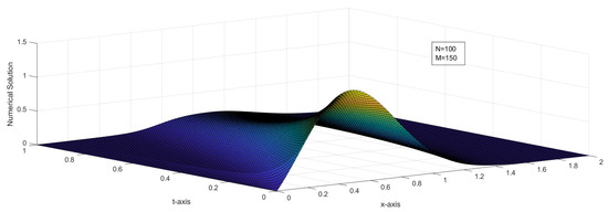
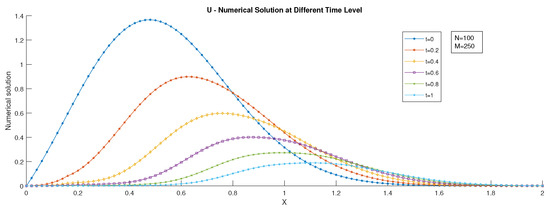
In this case, $\delta =1,\eta =1$ (symmetric delay arguments). Due to the presence of the delay term, an additional wave propagation occurs in the solutions. Numerical solutions are plotted in Figure 1 and Figure 2, and for different time levels, the solution curves are plotted in Figure 3 and Figure 4. The maximum pointwise error using the conditional method is given in Table 1, and for unconditional method, the errors are given in Table 2 and Table 3.

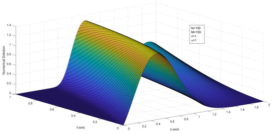Figure 1. The surface plot of the U–numerical solution of Example 1 for Case 1 using FTBS.

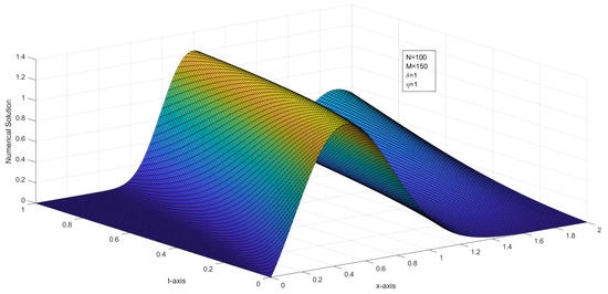Figure 2. The surface plot of the U–numerical solution of Example 1 for Case 1 using BTBS.

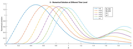Figure 3. U–numerical solution of Example 1 at different time levels for Case 1 using FTBS.

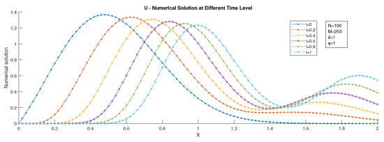Figure 4. U–numerical solution of Example 1 at different time levels for Case 1 using BTBS.

Table 1. Case 1: Maximum error for Example 1 using the conditional method.

	N and $\delta =1,\eta =1$
M ↓	64	128	256	512	1024
64	2.0649 × 10${}^{-2}$	2.1038 × 10${}^{-2}$	5.9393 × 10${}^{18}$	5.3383 × 10${}^{46}$	1.5500 × 10${}^{97}$
128	9.2118 × 10${}^{-3}$	7.4438 × 10${}^{-3}$	7.2246 × 10${}^{-3}$	5.8331 × 10${}^{40}$	1.5500 × 10${}^{97}$
256	4.3848 × 10${}^{-3}$	3.3665 × 10${}^{-3}$	2.6185 × 10${}^{-3}$	2.4920 × 10${}^{-3}$	3.2166 × 10${}^{85}$
512	2.1422 × 10${}^{-3}$	1.6116 × 10${}^{-3}$	1.1954 × 10${}^{-3}$	9.0767 × 10${}^{-4}$	8.6369 × 10${}^{-4}$
1024	1.0591 × 10${}^{-3}$	7.8936 × 10${}^{-4}$	5.7472 × 10${}^{-4}$	4.1630 × 10${}^{-4}$	3.1311 × 10${}^{-4}$

Table 2. Case 1: Maximum error for Example 1 using the unconditional method.

	N and $\delta =1,\eta =1$
M ↓	64	128	256	512	1024
64	1.4105 × 10${}^{-2}$	8.0063 × 10${}^{-3}$	4.4119 × 10${}^{-3}$	2.3598 × 10${}^{-3}$	1.2313 × 10${}^{-3}$
128	7.4588 × 10${}^{-3}$	4.3432 × 10${}^{-3}$	2.4755 × 10${}^{-3}$	1.3759 × 10${}^{-3}$	7.4200 × 10${}^{-4}$
256	3.8463 × 10${}^{-3}$	2.2792 × 10${}^{-3}$	1.3388 × 10${}^{-3}$	7.7517 × 10${}^{-4}$	4.3698 × 10${}^{-4}$
512	1.9545 × 10${}^{-3}$	1.1713 × 10${}^{-3}$	7.0246 × 10${}^{-4}$	4.2111 × 10${}^{-4}$	2.4858 × 10${}^{-4}$
1024	9.8540 × 10${}^{-4}$	5.9423 × 10${}^{-4}$	3.6097 × 10${}^{-4}$	2.2166 × 10${}^{-4}$	1.3595 × 10${}^{-4}$

Table 3. Case 3: Maximum error for Example 1 using the unconditional method.

	N and $\delta =1,\eta =0.5$
M ↓	64	128	256	512	1024
64	1.9072 × 10${}^{-2}$	1.3116 × 10${}^{-2}$	8.2844 × 10${}^{-3}$	4.8425 × 10${}^{-3}$	2.6635 × 10${}^{-3}$
128	1.0195 × 10${}^{-2}$	7.2773 × 10${}^{-3}$	4.8242 × 10${}^{-3}$	2.9639 × 10${}^{-3}$	1.7046 × 10${}^{-3}$
256	5.2854 × 10${}^{-3}$	3.8622 × 10${}^{-3}$	2.6482 × 10${}^{-3}$	1.7010 × 10${}^{-3}$	1.0281 × 10${}^{-3}$
512	2.6931 × 10${}^{-3}$	1.9944 × 10${}^{-3}$	1.3964 × 10${}^{-3}$	9.2669 × 10${}^{-4}$	5.8580 × 10${}^{-4}$
1024	1.3597 × 10${}^{-3}$	1.0140 × 10${}^{-3}$	7.1846 × 10${}^{-4}$	4.8675 × 10${}^{-4}$	3.1818 × 10${}^{-4}$

Case 2:

In this case, it is assumed that $\delta =0.5,\eta =0.5$ (symmetric delay arguments). The numerical solution is plotted in Figure 5, and the numerical solution at different time levels is presented in Figure 6.

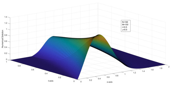Figure 5. The surface plot of the U–numerical solution of Example 1 for Case 2 using BTBS.

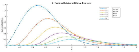Figure 6. U–numerical solution of Example 1 at different time levels for Case 2 using BTBS.

Case 3:

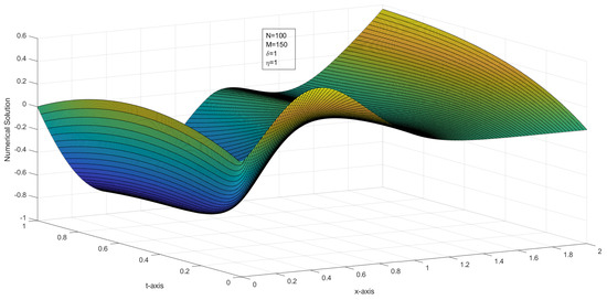
In this case, it is assumed that $\delta =1,\eta =0.5$ (asymmetric delay arguments). The numerical solution is plotted in Figure 7, and the numerical solution at different time levels is presented in Figure 8.

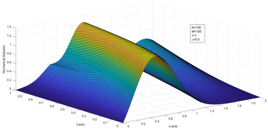Figure 7. The surface plot of the U–numerical solution of Example 1 for Case 3 using BTBS.

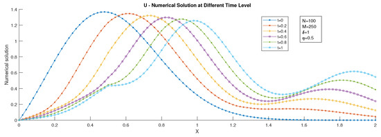Figure 8. U–numerical solution of Example 1 at different time levels for Case 3 using BTBS.

Example 2.

Consider the variable delay differential Equations (13)–(16).

where $a(x,t)={\displaystyle \frac{1+x^2}{1+2tx+2x^2+x^4}},$$b(x,t)=2,$$c(x,t)=-\frac{1}{2}$$d(x,t)=-\frac{1}{2}$, $\delta \left(x\right)=e^{-x}$, $\eta \left(x\right)=\sqrt{x}$. Figure 9 and Figure 10 respectively present the numerical solution and the numerical solution at different time levels.

Figure 9. U–numerical solution of Example 2 at different time levels using BTBS.

Figure 10. U–numerical solution of Example 2 at different time levels.

Example 3.

Consider the following first-order hyperbolic delay differential equation.

$$\begin{array}{cc}\hfill & \frac{\partial u}{\partial t}+a(x,t)\frac{\partial u}{\partial x}+bu(x,t)+c(x,t)u(x-\delta ,t)+d(x,t)u(x+\eta ,t)=0,(x,t)\in (0,2]\times (0,1],\hfill \end{array}$$

(22)

$$\begin{array}{cc}\hfill & u(x,t)=t-t^2+x{(2-x)}^2,(x,t)\in [-\delta ,0]\times [0,1],\hfill \end{array}$$

(23)

$$\begin{array}{cc}\hfill & u(x,t)=x{(2-x)}^2,(x,t)\in [x_f,x_f+\eta ]\times [0,1],\hfill \end{array}$$

(24)

$$\begin{array}{cc}\hfill & u(x,0)=xexp(-{(4x-1)}^2/4)(2-x),x\in [0,2],\hfill \end{array}$$

(25)

$$\begin{array}{c}\hfill a(x,t)={\displaystyle \frac{1+x^2}{1+2tx+2x^2+x^4}},b=2,c(x,t)=-\frac{1}{2},d(x,t)=-\frac{1}{2}.\end{array}$$

Figure 11 represents the numerical solutions of this problem.

Figure 11. U–numerical solution of Example 3 at different time levels using BTBS.

9. Conclusions

In this article, we considered a one-dimensional transport equation with delay and advance arguments. The maximum principle and stability results were proven for the problem considered. Two finite difference methods with piecewise linear interpolation were suggested for Problem (1)–(3). We proved that the methods are consistent and convergent of order one in space and time. One of the methods is conditionally stable, and the other one is unconditionally stable. The finite difference method with linear interpolation has some advantages. If $x_f\ne r\delta$, then one has to divided the interval $[0,x_f]$ into N sub-intervals with different mesh sizes. If $x_k\le x_i-\delta \le x_{k+1}$ and $x_p\le x_i+\eta \le x_{p+1}$, then one has to apply the interpolation of $U_k^j$, $U_{k+1}^j$ and $U_p^j$, $U_{p+1}^j$ to approximate $u(x_i-\delta ,t_j)$ and $u(x_i+\eta ,t_j).$ Numerical examples are given to illustrate the theoretical findings. The maximum pointwise errors of the examples are given in Table 1, Table 2, Table 3 and Table 4. From Table 1, one can see that Method (7)–(9) is conditionally stable, and from Table 2, Table 3 and Table 4, Method (10)–(12) is unconditionally stable. The newly proposed finite difference schemes with interpolation for the hyperbolic equation works not only for the constant delay and advanced arguments, but also for the variable arguments. As an application of the unconditionally stable method, a method for the variable delay equation is given in (17)–(18). A numerical example for variable delay equation is given in Example 2. The numerical solution and time level graphs are plotted in Figure 9 and Figure 10, respectively. The proposed method is applicable to the linear equation. The same method can be applied to some class of nonlinear equations after linearizing the given problem into a linear problem. Further, the proposed interpolation technique can be extended to the parabolic equation with delay arguments. As discussed in [10], for fixed $\delta$ and an increasing value of $\eta$, the impulse moves towards the left, whereas for the fixed $\eta$ and increasing value of $\delta$, the impulse moves towards the right; see Figure 12 and Figure 13.

Table 4. Maximum error for Example 3 using the unconditional method.

	N and $\delta =1,\eta =1$
M ↓	64	128	256	512	1024
64	1.7895 × 10${}^{-2}$	1.0976 × 10${}^{-2}$	8.5561 × 10${}^{-3}$	7.1527 × 10${}^{-3}$	6.1156 × 10${}^{-3}$
128	9.6501 × 10${}^{-3}$	6.1582 × 10${}^{-3}$	5.0506 × 10${}^{-3}$	4.4504 × 10${}^{-3}$	3.9743 × 10${}^{-3}$
256	5.0361 × 10${}^{-3}$	3.3007 × 10${}^{-3}$	2.8264 × 10${}^{-3}$	2.6236 × 10${}^{-3}$	2.4722 × 10${}^{-3}$
512	2.5753 × 10${}^{-3}$	1.7170 × 10${}^{-3}$	1.5124 × 10${}^{-3}$	1.4658 × 10${}^{-3}$	1.4578 × 10${}^{-3}$
1024	1.3027 × 10${}^{-3}$	8.7668 × 10${}^{-4}$	7.8569 × 10${}^{-4}$	7.8413 × 10${}^{-4}$	8.1491 × 10${}^{-4}$

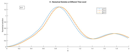
Figure 12. U–numerical solution of Example 1 at different time levels $\delta =1$ and $\eta =0.5,0.6,0.7$.

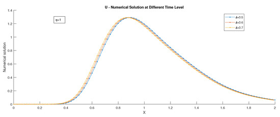
Figure 13. U–numerical solution of Example 1 at different time levels $\eta =1$ and $\delta =0.5,0.6,0.7$.

References

- Huang, C.; Vandewalle, S. An analysis of delay-dependent stability for ordinary and partial differential equations with fixed and distributed delays. SIAM J. Sci. Comput. 2004, 25, 1608–1632. [Google Scholar] [CrossRef]
- Huang, C.; Vandewalle, S. Unconditionally stable difference methods for delay partial differential equations. Numer. Math. 2012, 122, 579–601. [Google Scholar] [CrossRef]
- Kuang, Y. Delay Differential Equations with Applications in Population Dynamics; Academic Press: Cambridge, MA, USA, 1993; Volume 191. [Google Scholar]
- Hale, J.K.; Lunel, S.M.V.; Verduyn, L.S. Introduction to Functional Differential Equations; Springer: New York, NY, USA, 1993; Volume 10. [Google Scholar]
- Evans, L.C. Partial Differential Equations, 2nd ed.; American Mathematical Society: Providence, Rhode Island, 2010; Volume 19. [Google Scholar]
- Stein, R.B. A theoretical analysis of neuronal variability. Biophys. J. 1965, 5, 173–194. [Google Scholar] [CrossRef]
- Stein, R.B. Some models of neuronal variability. Biophys. J. 1967, 7, 37–68. [Google Scholar] [CrossRef]
- Ramesh, V.P.; Kadalbajoo, M.K. Upwind and midpoint upwind difference methods for time-dependent differential difference equations with layer behavior. Appl. Math. Comput. 2008, 202, 453–471. [Google Scholar] [CrossRef]
- Bansal, K.; Rai, P.; Sharma, K.K. Numerical treatment for the class of time dependent singularly perturbed parabolic problems with general shift arguments. Differ. Equ. Dyn. Syst. 2017, 25, 327–346. [Google Scholar] [CrossRef]
- Sharma, K.K.; Singh, P. Hyperbolic partial differential-difference equation in the mathematical modelling of neuronal firing and its numerical solution. Appl. Math. Comput. 2008, 201, 229–238. [Google Scholar] [CrossRef]
- Singh, P.; Sharma, K.K. Numerical solution of first-order hyperbolic partial differential-difference equation with shift. Numer. Methods Partial Differ. Equ. 2010, 26, 107–116. [Google Scholar] [CrossRef]
- Karthick, S.; Subburayan, V. Finite Difference Methods with Interpolation for First-Order Hyperbolic Delay Differential Equations. Springer Proc. Math. Stat. 2021, 368, 147–161. [Google Scholar]
- Collatz, L. The Numerical Treatment of Differential Equations, 3rd ed.; Springer: Berlin, Germany, 1966; Volume 60. [Google Scholar]
- Morton, K.W.; Mayers, D.F. Numerical Solution of Partial Differential Equations; Cambridge University Press: Cambridge, UK, 2005. [Google Scholar]
- Strikwerda, J.C. Finite Difference Schemes and Partial Differential Equations; SIAM: Philadelphia, PA, USA, 2004. [Google Scholar]
- Duffy, D.J. Finite Difference Methods in Financial Engineering: A Partial Differential Equation Approach; John Wiley and Sons: Hoboken, NJ, USA, 2013. [Google Scholar]
- Langtangen, H.P.; Linge, S. Finite Difference Computing with PDEs: A Modern Software Approach; Springer Nature: Berlin/Heidelberg, Germany, 2017. [Google Scholar]
- Mazumder, S. Numerical Methods for Partial Differential Equations: Finite Difference and Finite Volume Methods; Academic Press: Cambridge, MA, USA, 2015. [Google Scholar]
- Smith, G.D.; Smith, G.D.S. Numerical Solution of Partial Differential Equations: Finite Difference Methods; Oxford University Press: New York, NY, USA, 1985. [Google Scholar]
- Li, Z.; Qiao, Z.; Tang, T. Numerical Solution of Differential Equations: Introduction to Finite Difference and Finite Element Methods; Cambridge University Press: Cambridge, UK, 2018. [Google Scholar]
- Bellen, A.; Zennaro, M. Numerical Methods for Delay Differential Equations; Oxford University Press: Cambridge, UK, 2003. [Google Scholar]
- Al-Mutib, A.N. Stability properties of numerical methods for solving delay differential equations. J. Comput. Appl. Math. 1984, 10, 71–79. [Google Scholar] [CrossRef]
- Loustau, J. Numerical Differential Equations: Theory and Technique, ODE Methods, Finite Differences, Finite Elements and Collocation; World Scientific: Singapore, 2016. [Google Scholar]
- Warming, R.F.; Hyett, B.J. The modified equation approach to the stability and accuracy analysis of finite-difference methods. J. Comput. Phys. 1974, 14, 159–179. [Google Scholar] [CrossRef]
- Süli, E.; Mayers, D.F. An Introduction to Numerical Analysis; Cambridge University Press: Cambridge, UK, 2003. [Google Scholar]
- Protter, M.H.; Weinberger, H.F. Maximum Principles in Differential Equations; Springer: Berlin/Heidelberg, Germany, 1984. [Google Scholar]
- Bainov, D.D.; Kamont, Z.; Minchev, E. Comparison principles for impulsive hyperbolic equations of first order. J. Comput. Appl. Math. 1995, 60, 379–388. [Google Scholar] [CrossRef][Green Version]
- Liu, X.D. A maximum principle satisfying modification of triangle based adapative stencils for the solution of scalar hyperbolic conservation laws. SIAM J. Numer. Anal. 1993, 30, 701–716. [Google Scholar] [CrossRef]
- Selvi, P.A.; Ramanujam, N. An iterative numerical method for a weakly coupled system of singularly perturbed convection–diffusion equations with negative shifts. Int. J. Appl. Comput. Math. 2017, 3, 147–160. [Google Scholar] [CrossRef]
- Kalsoom, A.; Saleem, N.; Işık, H.; Al-Shami, T.M.; Bibi, A.; Khan, H. Fixed Point Approximation of Monotone Nonexpansive Mappings in Hyperbolic Spaces. J. Funct. Spaces 2021, 2021, 3243020 . [Google Scholar] [CrossRef]
- Saleem, N. Coincidence Best Proximity Point Results via wp-Distance with Applications. Metr. Fixed Point Theory 2021, 247–267. [Google Scholar]
- Lael, F.; Saleem, N.; Abbas, M. On the fixed points of multivalued mappings in b-metric spaces and their application to linear systems. UPB. Sci. Bull. 2020, 82, 121–130. [Google Scholar]
- Nie, L.; Mei, D. Effects of time delay on symmetric two-species competition subject to noise. Phys. Rev. E 2008, 77, 031107-1–031107-6. [Google Scholar] [CrossRef] [PubMed]
- Agarwal, R.P.; Chow, Y.M. Finite-difference methods for boundary-value problems of differential equations with deviating arguments. Comput. Method Appl. Math. 1986, 12, 1143–1153. [Google Scholar] [CrossRef]
- Jain, R.K.; Agarwal, R.P. Finite difference method for second order functional differential equations. J. Math. Phys. Sci. 1973, 7, 301–316. [Google Scholar]
Publisher’s Note: MDPI stays neutral with regard to jurisdictional claims in published maps and institutional affiliations. |
© 2022 by the authors. Licensee MDPI, Basel, Switzerland. This article is an open access article distributed under the terms and conditions of the Creative Commons Attribution (CC BY) license (https://creativecommons.org/licenses/by/4.0/).