Third-Order Tensor Decorrelation Based on 3D FO-HKLT with Adaptive Directional Vectorization

Abstract

In this work, we present a new hierarchical decomposition aimed at the decorrelation of a cubical tensor of size 2ⁿ, based on the 3D Frequency-Ordered Hierarchical KLT (3D FO-HKLT). The decomposition is executed in three consecutive stages. In the first stage, after adaptive directional vectorization (ADV) of the input tensor, the vectors are processed through one-dimensional FO-Adaptive HKLT (FO-AHKLT), and after folding, the first intermediate tensor is calculated. In the second stage, on the vectors obtained after ADV of the first intermediate tensor, FO-AHKLT is applied, and after folding, the second intermediate tensor is calculated. In the third stage, on the vectors obtained from the second intermediate tensor, ADV is applied, followed by FO-AHKLT, and the output tensor is obtained. The orientation of the vectors, calculated from each tensor, could be horizontal, vertical or lateral. The best orientation is chosen through analysis of their covariance matrix, based on its symmetry properties. The kernel of FO-AHKLT is the optimal decorrelating KLT with a matrix of size 2 × 2. To achieve higher decorrelation of the decomposition components, the direction of the vectors obtained after unfolding of the input tensor in each of the three consecutive stages, is chosen adaptively. The achieved lower computational complexity of FO-AHKLT is compared with that of the Hierarchical Tucker and Tensor Train decompositions.

1. Introduction

The main tensor decompositions could be divided into two groups.

The first group comprises decompositions executed in the spatial domain of the tensor. These are the famous Canonical Polyadic Decomposition (CPD), Higher-Order Singular Value Decomposition (HOSVD) [1,2,3,4], Tensor Train (TT) Decomposition [5], Hierarchical Tucker (H-Tucker) algorithm [6] and some of their modifications [7,8], based on the calculation of the tensor eigenvalues and eigenvectors. Their most important feature is that they are optimal regarding the minimization of the mean square approximation error derived from the low-energy component “truncation”. The calculation of the retained components is based on iterative methods [9,10] that need a relatively small number of mathematical operations to achieve the requested accuracy. The hierarchical tensor decompositions based on the H-Tucker algorithm are presented in publications [8,11]. The compositional hierarchical tensor factorization introduced in [8] disentangles the hierarchical causal structure of object image formation, but the computational complexity (or Complexity) is not presented. In [11] is offered the TT-based hierarchical decomposition of high-order tensors, based on the Tensor-Train Hierarchical SVD (TT-HSVD). This approach permits parallel processing, which significantly accelerates the process. Unlike the TT-SVD algorithm, TT-HSVD is based on applying SVDs to matrices of smaller dimensions, which results in lower Complexity of TT-HSVD.

The second group comprises tensor decompositions performed in the transform domain, which use reversible 3D linear orthogonal transforms such as the Fast Fourier Transform (FFT), Discrete Cosine Transform (DCT), etc. [12,13,14]. This approach is distinguished by its flexibility regarding the choice of the transform based on the processed data contents.

In this work, we present alternative new hierarchical 3D tensor decompositions based on the famous statistical orthogonal Karhunen–Loeve Transform (KLT) [15,16]. They are close to optimal (which ensures full decorrelation of the decomposition components), but do not need iterations and have lower computational complexity. As a basis, we present here the decomposition called 3D Frequency-Ordered Adaptive Hierarchical Karhunen–Loeve Transform (3D FO-AHKLT), whose efficiency is enhanced through adaptive directional tensor vectorization (ADV).

In Section 2, we present the method for 3D hierarchical adaptive transform based on the one-dimensional Frequency-Ordered Adaptive Hierarchical Karhunen–Loeve Transform (FO-AHKLT). Section 3 gives the details on the cubical tensor decomposition through separable 3D FO-AHKLT based on correlation analysis, and Section 4 explains the related algorithm. In Section 5, we analyze the computational complexity of the new approaches compared to that of the well-known H-Tucker and TT decompositions; Section 6 contains the conclusion.

2. Method for 3D Adaptive Frequency-Ordered Hierarchical KLT of a Cubical Tensor

The proposed method for decomposition of 3rd order cubical tensor $\mathbf{𝒳}\in {\mathrm{R}}^{\mathrm{N}\times \mathrm{N}\times \mathrm{N}}$ is based on the 3D Frequency-Ordered Hierarchical Karhunen–Loeve Transform (3D FO-HKLT), defined by the relation below [17]:

$$\mathbf{𝒳}=(1/{\mathrm{N}}^3){\displaystyle \sum _{\mathrm{m}=0}^{\mathrm{N}-1}{\displaystyle \sum _{v=0}^{\mathrm{N}-1}{\displaystyle \sum _{l=0}^{\mathrm{N}-1}\mathrm{s}(\mathrm{m},\mathrm{v},\mathrm{l})[k_{\mathrm{m}}(1)\circ k_{\mathrm{v}}(2)\circ k_{\mathrm{l}}(3)]}}}.$$

(1)

Here, N = 2ⁿ is the size of the tensor $\mathbf{𝒳}$ with nonnegative components x (i, j, k). The coefficients $\mathrm{s}(\mathrm{m},\mathrm{v},\mathrm{l})$ are the elements of the spectrum tensor S, which is of the same size as $\mathbf{𝒳}$. Each coefficient $\mathrm{s}(\mathrm{m},\mathrm{v},\mathrm{l})$ represents the weights of the basic tensor, ${\mathbf{𝒦}}_{\mathrm{u},\mathrm{v},\mathrm{l}}$. Each basic tensor is represented as the outer product of three vectors:

$${\mathbf{𝒦}}_{\mathrm{m},\mathrm{v},\mathrm{l}}=k_{\mathrm{n}}(1)\circ k_{\mathrm{v}}(2)\circ k_{\mathrm{l}}(3).$$

(2)

Here, “$\circ$” denotes the outer product of the two column-vectors $(x\circ y=x·y^{\mathrm{T}})$, and $k_{\mathrm{m}}(1),k_{\mathrm{v}}(2),k_{\mathrm{l}}(3)$ are the basic vectors, obtained after execution of the three stages of 3D FO-HKLT. In the first decomposition components $\mathrm{s}(\mathrm{m},\mathrm{v},\mathrm{l}).{\mathbf{𝒦}}_{\mathrm{m},\mathrm{v},\mathrm{l}}$ (as given in Equation (1)) the main part of the tensor $\mathbf{𝒳}$ power is concentrated, and their high decorrelation is achieved. The kernel of 3D FO-HKLT, defined as KLT_2×2, is KLT with a transform matrix of size 2 × 2.

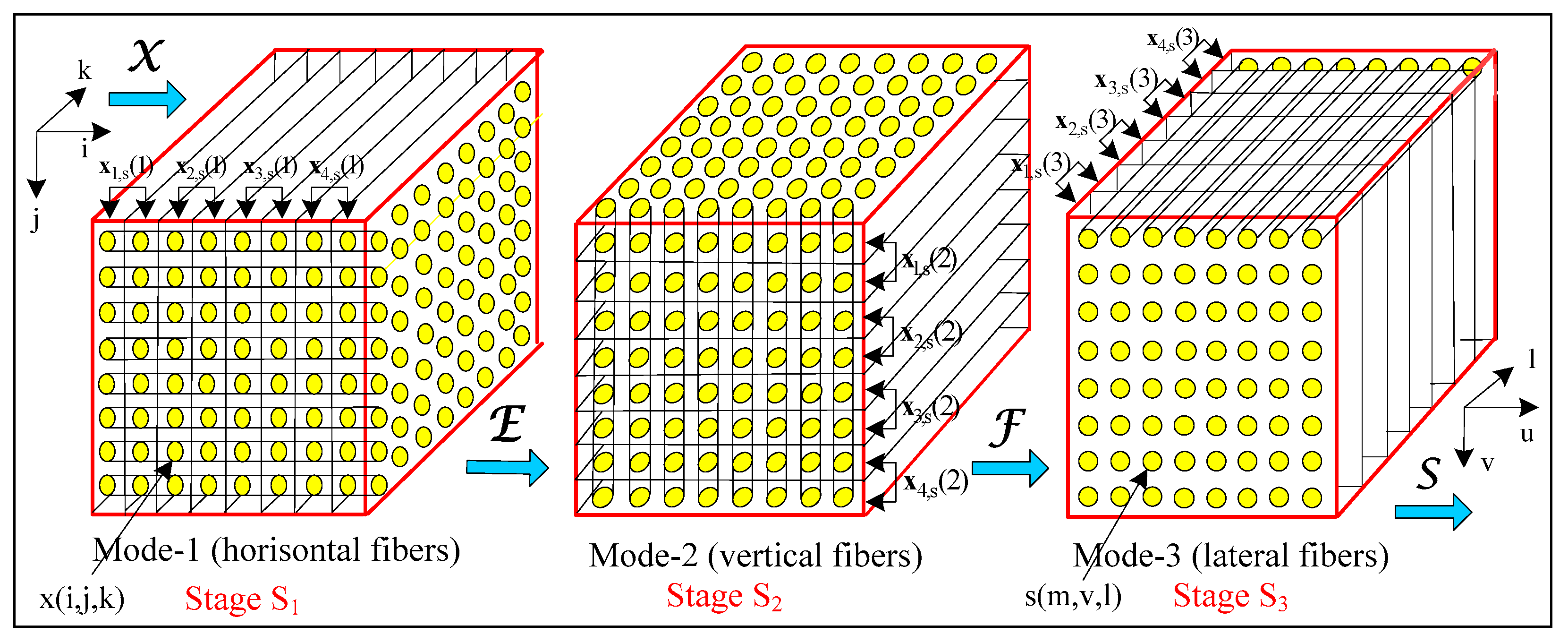
The decomposition comprises three consecutive stages arranged in accordance with the correlation analysis of the tensor $\mathbf{𝒳}$ elements. One example decomposition for the tensor X of size N × N × N (for N = 8) is shown in Figure 1. After applying the 3D FO-AHKLT on the input tensor X, it is sequentially transformed into the intermediate tensors E, F and the output tensor, S. The 3D FO-AHKLT is divisible, and this permits it to be executed by using the FO-AHKLT, whose graph for the case N = 8 is shown in Figure 2. As a result, the tensor $\mathbf{𝒳}$ is transformed into the first intermediate tensor E, of the same size.

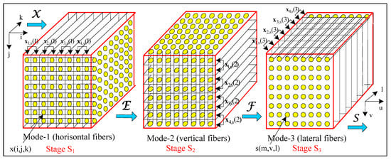
Figure 1. Sequence of the 3D FO-AHKLT execution stages for a tensor $\mathbf{𝒳}$ of size 8 × 8 × 8 for the case. Δ (1) > Δ (2) > Δ (3), based on FO-AHKLT. On each 2-component $x_{\mathrm{q},\mathrm{s}}(\mathrm{u})$ for q = 1, 2, 3, 4, KLT_2×2 is applied.

Figure 2. Graphs of the 3-level direct FO-AHKLT of the tensor X of size 8 × 8 × 8, with ADV.

In the general case, FO-HKLT is executed for the N-dimensional vectors $x_{\mathrm{s}}(\mathrm{u})$ of total number N², oriented in horizontal (u = 1), vertical (u = 2) or lateral (u = 3) direction. These vectors are defined as a result of the ADV of the tensor $\mathbf{𝒳}$. The choice of the orientation direction of vectors $x_{\mathrm{s}}(\mathrm{u})$ for s = 1, 2, …, N² is defined through analysis of their covariance matrices, K_x(u). Before the calculation of FO-HKLT for the N-dimensional vector $x_{\mathrm{s}}(\mathrm{u})$, it is divided into N/2 two-component vectors $x_{\mathrm{q},\mathrm{s}}(\mathrm{u})$. For the case N = 8, each vector $x_{\mathrm{s}}(\mathrm{u})$ is divided into 4 vectors $x_{\mathrm{q},\mathrm{s}}(\mathrm{u})$, for q = 1, 2, 3, 4. For this case, the total number of vectors $x_{\mathrm{s}}(\mathrm{u})$ is 4N² = 256, and they are divided into 4 sub-groups of N² = 64 vectors $x_{\mathrm{q},\mathrm{s}}(\mathrm{u})$ each.

Let $x_{\mathrm{s}}={[{\mathrm{x}}_{1,\mathrm{s}},{\mathrm{x}}_{2,\mathrm{s}},\dots ,{\mathrm{x}}_{\mathrm{n},\mathrm{s}}]}^{\mathrm{T}}$ and $e_{\mathrm{s}}={[{\mathrm{e}}_{1,\mathrm{s}},{\mathrm{e}}_{2,\mathrm{s}},\dots ,{\mathrm{e}}_{\mathrm{N},\mathrm{s}}]}^{\mathrm{T}}$ be the input and the output column-vectors of N = 2ⁿ components, respectively, and n is the number of FO-HKLT hierarchical levels. The relation between vectors e_s and x_s, is [17]:

$$e_{\mathrm{s}}=P_{\mathrm{n}}{(2}^{\mathrm{n}})[{\displaystyle \prod _{\mathrm{p}=1}^{\mathrm{n}}{G}_{\mathrm{p}} {(2}^{\mathrm{n}})}] x_{\mathrm{s}}=T_{\mathrm{FO}-\mathrm{HKLT}}(2^{\mathrm{n}})x_{\mathrm{s}} \mathrm{for} \mathrm{s}=1, 2, \dots , {\mathrm{N}}^2,$$

(3)

where $T_{\mathrm{FO}-\mathrm{HKLT}} (2^{\mathrm{n}})=P_{\mathrm{n}}(2^{\mathrm{n}})[{\displaystyle \prod _{\mathrm{p}=1}^{\mathrm{n}}{G}_{\mathrm{p}} {(2}^{\mathrm{n}})}]$ is the FO-HKLT matrix; $P_{\mathrm{n}}(2^{\mathrm{n}})$ of size 2ⁿ × 2ⁿ is the permutation matrix for the last level n of FO-HKLT, and ${\displaystyle \prod _{\mathrm{p}=1}^{\mathrm{n}}{G}_{\mathrm{p}} {(2}^{\mathrm{n}})}$ is the product of n sparse transform matrices $G_{\mathrm{p}}(2^{\mathrm{n}})$ for p = 1, 2, 3, …, n. Each matrix $G_{\mathrm{p}}(2^{\mathrm{n}})$ is defined as follows:

$$G_{\mathrm{p}}(2^{\mathrm{n}})=\left[\begin{array}{cc}\underset{\mathrm{j}=1}{\overset{2^{\mathrm{p}-1}}{\oplus }}{\mathrm{c}}_{\mathrm{p},\mathrm{j}}& \underset{\mathrm{j}=1}{\overset{2^{\mathrm{p}-1}}{\oplus }}{\mathrm{s}}_{\mathrm{p},\mathrm{j}}\\ \underset{\mathrm{j}=1}{\overset{2^{\mathrm{p}-1}}{\oplus }}{\mathrm{s}}_{\mathrm{p},\mathrm{j}}& \underset{\mathrm{j}=1}{\overset{2^{\mathrm{p}-1}}{\oplus }}-{\mathrm{c}}_{\mathrm{p},\mathrm{j}}\end{array}\right]\oplus \left[\begin{array}{cc}\underset{\mathrm{j}=1}{\overset{2^{\mathrm{p}-1}}{\oplus }}{\mathrm{c}}_{{\mathrm{p},2}^{\mathrm{p}-1}+\mathrm{j}}& \underset{\mathrm{j}=1}{\overset{2^{\mathrm{p}-1}}{\oplus }}{\mathrm{s}}_{{\mathrm{p},2}^{\mathrm{p}-1}+\mathrm{j}}\\ \underset{\mathrm{j}=1}{\overset{2^{\mathrm{p}-1}}{\oplus }}{\mathrm{s}}_{{\mathrm{p},2}^{\mathrm{p}-1}+\mathrm{j}}& \underset{\mathrm{j}=1}{\overset{2^{\mathrm{p}-1}}{\oplus }}-{\mathrm{c}}_{{\mathrm{p},2}^{\mathrm{p}-1}+\mathrm{j}}\end{array}\right]\oplus \dots \oplus \left[\begin{array}{cc}\underset{\mathrm{j}=1}{\overset{2^{\mathrm{p}-1}}{\oplus }}{\mathrm{c}}_{{\mathrm{p},2}^{\mathrm{p}-1}(\mathrm{n}-\mathrm{p}-1)+\mathrm{j}}& \underset{\mathrm{j}=1}{\overset{2^{\mathrm{p}-1}}{\oplus }}{\mathrm{s}}_{{\mathrm{p},2}^{\mathrm{p}-1}(\mathrm{n}-\mathrm{p}-1)+\mathrm{j}}\\ \underset{\mathrm{j}=1}{\overset{2^{\mathrm{p}-1}}{\oplus }}{\mathrm{s}}_{{\mathrm{p},2}^{\mathrm{p}-1}(\mathrm{n}-\mathrm{p}-1)+\mathrm{j}}& \underset{\mathrm{j}=1}{\overset{2^{\mathrm{p}-1}}{\oplus }}-{\mathrm{c}}_{{\mathrm{p},2}^{\mathrm{p}-1}(\mathrm{n}-\mathrm{p}-1)+\mathrm{j}}\end{array}\right]$$

(4)

for p = 1, 2, 3, …, n, where “⊕” denotes the direct sum of matrices.

In the equations, figures and text below, the abbreviations ${\mathrm{c}}_{\mathrm{p},\mathrm{q}}=\cos {\mathsf{\theta }}_{\mathrm{p},\mathrm{q}}$ and ${\mathrm{s}}_{\mathrm{p},\mathrm{q}}={\sin \mathsf{\theta }}_{\mathrm{p},\mathrm{q}}$ are used. Here:

$${\mathsf{\theta }}_{\mathrm{p},\mathrm{q}}=\arctan \{2{\mathrm{k}}_3(\mathrm{p},\mathrm{q})/[{\mathrm{k}}_1(\mathrm{p},\mathrm{q})-{\mathrm{k}}_2(\mathrm{p},\mathrm{q})+\sqrt{{({\mathrm{k}}_1(\mathrm{p},\mathrm{q})-{\mathrm{k}}_2(\mathrm{p},\mathrm{q}))}^2+4{\mathrm{k}}_3^2(\mathrm{p},\mathrm{q})}]\},$$

(5)

$${\mathrm{k}}_1(\mathrm{p},\mathrm{q})=\mathrm{E}\{{\mathrm{x}}_{1,\mathrm{s}}^2(\mathrm{p},\mathrm{q})\}; {\mathrm{k}}_2(\mathrm{p},\mathrm{q})=\mathrm{E}\{{\mathrm{x}}_{2,\mathrm{s}}^2(\mathrm{p},\mathrm{q})\}; {\mathrm{k}}_3(\mathrm{p},\mathrm{q})=\mathrm{E}\{{\mathrm{x}}_{1,\mathrm{s}}(\mathrm{p},\mathrm{q}){\mathrm{x}}_{2,\mathrm{s}}(\mathrm{p},\mathrm{q})\}.$$

(6)

$\mathrm{E}\{{\mathrm{x}}_{\mathrm{i},\mathrm{s}}(\mathrm{p},\mathrm{q})\}=(1/{\mathrm{N}}^2){\displaystyle \sum _{\mathrm{s}=1}^{{\mathrm{N}}^2}{\mathrm{x}}_{\mathrm{i},\mathrm{s}}(\mathrm{p},\mathrm{q})}$ for i = 1, 2-averaging operator.

If β₂ = 2k₃(p,q) and ${\mathsf{\beta }}_1={\mathrm{k}}_1(\mathrm{p},\mathrm{q})-{\mathrm{k}}_2(\mathrm{p},\mathrm{q})+\sqrt{{{[\mathrm{k}}_1(\mathrm{p},\mathrm{q})-{\mathrm{k}}_2(\mathrm{p},\mathrm{q})]}^2+{4\mathrm{k}}_3^2(\mathrm{p},\mathrm{q})}$ are two real numbers, the extended arctan function ε_arctan (β₁,β₂) is mapped to (−π, π] by adding π [18]:

$${\mathsf{\epsilon }}_{\arctan }({\mathsf{\beta }}_1,{\mathsf{\beta }}_2)=\{\begin{array}{ccc}{\arctan (\mathsf{\beta }}_2/{\mathsf{\beta }}_1),\hfill & \mathrm{if}\hfill & \hfill {\mathsf{\beta }}_1>0;\\ {\arctan (\mathsf{\beta }}_2/{\mathsf{\beta }}_1)+\mathsf{\pi },\hfill & \mathrm{if}\hfill & \hfill {\mathsf{\beta }}_1<{0, \mathsf{\beta }}_2\ge 0;\\ {\arctan (\mathsf{\beta }}_2/{\mathsf{\beta }}_1)-\mathsf{\pi },\hfill & \mathrm{if}\hfill & \hfill {\mathsf{\beta }}_1<{0, \mathsf{\beta }}_2<0;\\ \mathsf{\pi }/2,\hfill & \mathrm{if}\hfill & \hfill {\mathsf{\beta }}_1={0, \mathsf{\beta }}_2>0;\\ -\mathsf{\pi }/2,\hfill & \mathrm{if}\hfill & \hfill {\mathsf{\beta }}_1={0, \mathsf{\beta }}_2<0;\\ 0,\hfill & \mathrm{if}\hfill & \hfill {\mathsf{\beta }}_2={\mathsf{\beta }}_1=0.\end{array}$$

(7)

In particular, the direct and inverse KLT_2×2 of the elements x_1s and x_2s, which have the same spatial position in the couple of matrices X₁ and X₂ of size N × N for ${\mathrm{m}}_1=\mathrm{E}\left\{{\mathrm{x}}_{1\mathrm{s}}\right\}=0$ and ${\mathrm{m}}_2=\mathrm{E}\left\{{\mathrm{x}}_{2\mathrm{s}}\right\}=0$ (valid for the Adaptive KLT_2×2), are:

$${\mathrm{y}}_{1\mathrm{s}}={\mathrm{x}}_{1\mathrm{s}}{\cos \mathsf{\theta }}_{1,2}+{\mathrm{x}}_{2\mathrm{s}}{\sin \mathsf{\theta }}_{1,2};{\mathrm{x}}_{1\mathrm{s}}={\mathrm{y}}_{1\mathrm{s}}{\cos \mathsf{\theta }}_{1,2}+{\mathrm{y}}_{2\mathrm{s}}{\sin \mathsf{\theta }}_{1,2};$$

(8)

$${\mathrm{y}}_{2\mathrm{s}}={\mathrm{x}}_{1\mathrm{s}}{\sin \mathsf{\theta }}_{1,2}-{\mathrm{x}}_{2\mathrm{s}}{\cos \mathsf{\theta }}_{1,2};{\mathrm{x}}_{2\mathrm{s}}={\mathrm{y}}_{1\mathrm{s}}{\sin \mathsf{\theta }}_{1,2}-{\mathrm{y}}_{2\mathrm{s}}{\cos \mathsf{\theta }}_{1,2}.$$

(9)

or $y_{\mathrm{s}}=T(2)·x_{\mathrm{s}}$ and $x_{\mathrm{s}}=T(2)·y_{\mathrm{s}}$ for s = 1, 2, …, N².

Here, y_1s and y_2s are the corresponding elements in the couple of transformed matrices Y₁ and Y₂ (each of size N × N); $y_{\mathrm{s}}={[{\mathrm{y}}_{1,\mathrm{s}},{\mathrm{y}}_{2,\mathrm{s}}]}^{\mathrm{T}}$, $x_{\mathrm{s}}={[{\mathrm{x}}_{1,\mathrm{s}},{\mathrm{x}}_{2,\mathrm{s}}]}^{\mathrm{T}}$ and $[T(2)]=\left[\begin{array}{cc}{\cos \mathsf{\theta }}_{1,2}& {\sin \mathsf{\theta }}_{1,2}\\ {\sin \mathsf{\theta }}_{1,2}& {-\cos \mathsf{\theta }}_{1,2}\end{array}\right]=\left[\begin{array}{cc}{\mathrm{c}}_{1,2}& {\mathrm{s}}_{1,2}\\ {\mathrm{s}}_{1,2}& {-\mathrm{c}}_{1,2}\end{array}\right]$.

In particular, for ${\mathsf{\theta }}_{1,2}=\mathsf{\pi }/4$, the relations (8) and (9) become as follows:

$$\begin{array}{l}{\mathrm{y}}_{1\mathrm{s}}=({\mathrm{x}}_{1\mathrm{s}}+{\mathrm{x}}_{2\mathrm{s}});\\ {\mathrm{y}}_{2\mathrm{s}}=({\mathrm{x}}_{1\mathrm{s}}-{\mathrm{x}}_{2\mathrm{s}});\end{array}\dots \begin{array}{l}{\mathrm{x}}_{1\mathrm{s}}=(1/2)({\mathrm{y}}_{1\mathrm{s}}+{\mathrm{y}}_{2\mathrm{s}});\\ {\mathrm{x}}_{2\mathrm{s}}=(1/2)({\mathrm{y}}_{1\mathrm{s}}-{\mathrm{y}}_{2\mathrm{s}}).\end{array}$$

(10)

Hence, in this case, the KLT_2×2 coincides with the Walsh–Hadamard Transform (WHT).

In the level n, the components of the column-vectors $y_{\mathrm{n},\mathrm{s}}=G_{\mathrm{n}}(2^{\mathrm{n}})y_{\mathrm{n}-1,\mathrm{s}}$ (respectively, the components of matrices Y_n,k for k = 0, 1, …, N − 1) are rearranged. For this, the permutation matrix $P_{\mathrm{n}}(2^{\mathrm{n}})$ is used.

From the components of the column-vectors $e_{\mathrm{s}}=P_{\mathrm{n}}(2^{\mathrm{n}})y_{\mathrm{n},\mathrm{s}}$ are obtained the frequency-ordered matrices E_r (i.e., E₀, E₁, …, E_N−1), calculated in accordance with the relation between their sequential number r and the sequential number k (for matrices Y_n,k).

The relation that defines the matrix $P_{\mathrm{n}}(2^{\mathrm{n}})$ is:

• The binary code ${\mathrm{k}}_{\mathrm{n}-1}{,\mathrm{k}}_{\mathrm{n}-2},\dots {,\mathrm{k}}_0$ of the sequential decimal number k = 0, 1, …, 2ⁿ⁻¹ of the component Y_n,k is arranged inversely (i.e., ${\mathrm{k}}_0{,\mathrm{k}}_1,\dots {,\mathrm{k}}_{\mathrm{n}-1}$), as ${\mathrm{g}}_{\mathrm{i}}={\mathrm{k}}_{\mathrm{n}-\mathrm{i}-1}$ for 0 ≤ i ≤ n − 1;
• The so-obtained code ${\mathrm{g}}_{\mathrm{n}-1}{,\mathrm{g}}_{\mathrm{n}-2},\dots {,\mathrm{g}}_0$ is transformed from Gray code into the binary code ${\mathrm{r}}_{\mathrm{n}-1}{,\mathrm{r}}_{\mathrm{n}-2},\dots {,\mathrm{r}}_0$, in accordance with the operations ${\mathrm{r}}_{\mathrm{n}-1}={\mathrm{g}}_{\mathrm{n}-1},{\mathrm{r}}_{\mathrm{i}}={\mathrm{r}}_{\mathrm{i}-1}\oplus {\mathrm{g}}_{\mathrm{i}}$ for 0 ≤ i ≤ n − 2. Here, “⊕” denotes the operation “exclusive OR”.

The decimal number $\mathrm{r}={\displaystyle \sum _{\mathrm{i}=0}^{\mathrm{n}-1}{\mathrm{r}}_{\mathrm{i}}}{2}^{\mathrm{i}}$ defines the sequential number of E_r for r = 0, 1, …, 2ⁿ⁻¹, which (before the rearrangement) corresponded to Y_n,_k, with sequential number $\mathrm{k}={\displaystyle \sum _{\mathrm{i}=0}^{\mathrm{n}-1}{\mathrm{k}}_{\mathrm{i}}}{2}^{\mathrm{i}}$.

For N = 8 (n = 3), p = 1, 2, 3 and q = 1, 2, 3, 4, FO-HKLT is executed in three consecutive levels. The transform matrix of size 8 × 8 is decomposed in accordance with the relation:

$$T_{\mathrm{FO}-\mathrm{HKLT}}(8)=P_3(8)G_3(8)G_2(8)G_1(8)$$

(11)

Since $e_{\mathrm{s}}=P_3(8)G_3(8)G_2(8)G_1(8)x_{\mathrm{s}}$, the transform is executed as follows:

$$y_{1,\mathrm{s}}=G_1(8)x_{\mathrm{s}}, y_{2,\mathrm{s}}=G_2(8)y_{1,\mathrm{s}}, y_{3,\mathrm{s}}=G_3(8)y_{2,\mathrm{s}}, e_{\mathrm{s}}=P_3(8)y_{3,\mathrm{s}}$$

(12)

The operations above correspond to the calculations in hierarchical levels p = 1, 2, 3 of FO-HKLT. In this case, the transform matrices $G_1(8), G_2(8), G_3(8)$ are defined by the equations:

$$G_1(8)=\left[\begin{array}{cccccccc}{\mathrm{c}}_{1,1}& {\mathrm{s}}_{1,1}& 0& 0& 0& 0& 0& 0\\ {\mathrm{s}}_{1,1}& -{\mathrm{c}}_{1,1}& 0& 0& 0& 0& 0& 0\\ 0& 0& {\mathrm{c}}_{1,2}& {\mathrm{s}}_{1,2}& 0& 0& 0& 0\\ 0& 0& {\mathrm{s}}_{1,2}& -{\mathrm{c}}_{1,2}& 0& 0& 0& 0\\ 0& 0& 0& 0& {\mathrm{c}}_{1,3}& {\mathrm{s}}_{1,3}& 0& 0\\ 0& 0& 0& 0& {\mathrm{s}}_{1,3}& -{\mathrm{c}}_{1,3}& 0& 0\\ 0& 0& 0& 0& 0& 0& {\mathrm{c}}_{1,4}& {\mathrm{s}}_{1,4}\\ 0& 0& 0& 0& 0& 0& {\mathrm{s}}_{1,4}& -{\mathrm{c}}_{1,4}\end{array}\right]$$

(13)

where ${\mathsf{\theta }}_{1,\mathrm{q}}=\arctan \{2{\mathrm{k}}_3(1,\mathrm{q})/[{\mathrm{k}}_1(1,\mathrm{q})-{\mathrm{k}}_2(1,\mathrm{q})+\sqrt{{({\mathrm{k}}_1(1,\mathrm{q})-{\mathrm{k}}_2(1,\mathrm{q}))}^2+4{\mathrm{k}}_3^2(1,\mathrm{q})}]\}$ for q = 1, 2, 3, 4 and p = 1; ${\mathrm{k}}_1(1,\mathrm{q})=\mathrm{E}\{{\mathrm{x}}_{1,\mathrm{s}}^2(1,\mathrm{q})\};$ ${\mathrm{k}}_2(\mathrm{p},\mathrm{q})=\mathrm{E}\{{\mathrm{x}}_{2,\mathrm{s}}^2(1,\mathrm{q})\};$ ${\mathrm{k}}_3(1,\mathrm{q})=\mathrm{E}\{{\mathrm{x}}_{1,\mathrm{s}}(1,\mathrm{q})·{\mathrm{x}}_{2,\mathrm{s}}(1,\mathrm{q})\}.$

$$G_2(8)=\left[\begin{array}{cccccccc}{\mathrm{c}}_{2,1}& 0& {\mathrm{s}}_{2,1}& 0& 0& 0& 0& 0\\ 0& {\mathrm{c}}_{2,2}& 0& {\mathrm{s}}_{2,2}& 0& 0& 0& 0\\ {\mathrm{s}}_{2,1}& 0& {-\mathrm{c}}_{2,1}& 0& 0& 0& 0& 0\\ 0& {\mathrm{s}}_{2,2}& 0& -{\mathrm{c}}_{2,2}& 0& 0& 0& 0\\ 0& 0& 0& 0& {\mathrm{c}}_{2,3}& 0& {\mathrm{s}}_{2,3}& 0\\ 0& 0& 0& 0& 0& {\mathrm{c}}_{2,4}& 0& {\mathrm{s}}_{2,4}\\ 0& 0& 0& 0& {\mathrm{s}}_{2,3}& 0& {-\mathrm{c}}_{2,3}& 0\\ 0& 0& 0& 0& 0& {\mathrm{s}}_{2,4}& 0& -{\mathrm{c}}_{2,4}\end{array}\right]$$

(14)

where: ${\mathsf{\theta }}_{2,\mathrm{q}}=\arctan \{2{\mathrm{k}}_3(2,\mathrm{q})/[{\mathrm{k}}_1(2,\mathrm{q})-{\mathrm{k}}_2(2,\mathrm{q})+\sqrt{{({\mathrm{k}}_1(2,\mathrm{q})-{\mathrm{k}}_2 (2,\mathrm{q}))}^2+4{\mathrm{k}}_3^2(2,\mathrm{q})}]\}$ for q = 1, 2, 3, 4 and p = 2; ${\mathrm{k}}_1(2,\mathrm{q})=\mathrm{E}\{{\mathrm{y}}_{1,1\mathrm{s}}^2(2,\mathrm{q})\};$ ${\mathrm{k}}_2(2,\mathrm{q})=\mathrm{E}\{{\mathrm{y}}_{1,2\mathrm{s}}^2(2,\mathrm{q})\};$ ${\mathrm{k}}_3(2,\mathrm{q})=\mathrm{E}\{{\mathrm{y}}_{1,1\mathrm{s}}(2,\mathrm{q})·{\mathrm{y}}_{1,2\mathrm{s}}(2,\mathrm{q})\}.$

$$G_3(8)=\left[\begin{array}{cccccccc}{\mathrm{c}}_{3,1}& 0& 0& 0& {\mathrm{s}}_{3,1}& 0& 0& 0\\ 0& {\mathrm{c}}_{3,2}& 0& 0& 0& {\mathrm{s}}_{3,2}& 0& 0\\ 0& 0& {\mathrm{c}}_{3,3}& 0& 0& 0& {\mathrm{s}}_{3,3}& 0\\ 0& 0& 0& {\mathrm{c}}_{3,4}& 0& 0& 0& {\mathrm{s}}_{3,4}\\ {\mathrm{s}}_{3,1}& 0& 0& 0& {-\mathrm{c}}_{3,1}& 0& 0& 0\\ 0& {\mathrm{s}}_{3,2}& 0& 0& 0& -{\mathrm{c}}_{3,2}& 0& 0\\ 0& 0& {\mathrm{s}}_{3,3}& 0& 0& 0& {-\mathrm{c}}_{3,3}& 0\\ 0& 0& 0& {\mathrm{s}}_{3,4}& 0& 0& 0& -{\mathrm{c}}_{3,4}\end{array}\right]$$

(15)

where ${\mathsf{\theta }}_{3,\mathrm{q}}=\arctan \{2{\mathrm{k}}_3(3,\mathrm{q})/[{\mathrm{k}}_1(3,\mathrm{q})-{\mathrm{k}}_2(1,\mathrm{q})+\sqrt{{({\mathrm{k}}_1(3,\mathrm{q})-{\mathrm{k}}_2(3,\mathrm{q}))}^2+4{\mathrm{k}}_3^2(3,\mathrm{q})}]\}$ for q = 1, 2, 3, 4 and p = 3; ${\mathrm{k}}_1(3,\mathrm{q})=\mathrm{E}\{{\mathrm{y}}_{2,1,\mathrm{s}}^2(3,\mathrm{q})\};$ ${\mathrm{k}}_2(3,\mathrm{q})=\mathrm{E}\{{\mathrm{y}}_{2,2,\mathrm{s}}^2(3,\mathrm{q})\};$ ${\mathrm{k}}_3(3,\mathrm{q})=\mathrm{E}\{{\mathrm{y}}_{2,1,\mathrm{s}}(3,\mathrm{q})-{\mathrm{y}}_{2,2,\mathrm{s}}(3,\mathrm{q})\}$.

The permutation matrix $P_3(8)$ in the level p = 3 is:

$$P_3(8)=\left[\begin{array}{cccccccc}1& 0& 0& 0& 0& 0& 0& 0\\ 0& 0& 0& 0& 1& 0& 0& 0\\ 0& 0& 0& 0& 0& 0& 1& 0\\ 0& 0& 1& 0& 0& 0& 0& 0\\ 0& 0& 0& 1& 0& 0& 0& 0\\ 0& 0& 0& 0& 0& 0& 0& 1\\ 0& 0& 0& 0& 0& 1& 0& 0\\ 0& 1& 0& 0& 0& 0& 0& 0\end{array}\right]$$

(16)

The vector $k_{\mathrm{m}}(1)$ for m = 0, 1, …, 7 comprises the elements of the mth row of the matrix $T_{\mathrm{FO}-\mathrm{HKLT}}^1(8)$ for the stage S₁ of 3D FO-HKLT. The vectors $k_{\mathrm{v}}(2)$ and $k_{\mathrm{l}}(3)$ for v, l = 0, 1, …, 7 respectively comprise the elements of rows v and l in matrices $T_{\mathrm{FO}-\mathrm{HKLT}}^2(8)$ and $T_{\mathrm{FO}-\mathrm{HKLT}}^3(8)$, for 3D FO-HKLT stages S₂ and S₃.

3. Enhancement of the 3D FO-HKLT Efficiency, Based on Correlation Analysis

To achieve higher efficiency of the 3D tensor decomposition based on the 3D FO-HKLT, here, we use the correlation relations between the tensor $\mathbf{𝒳}$ components in the orthogonal directions x, y, z. To detect the direction in which these relations are strongest, correlation analysis should be used. It is based on the analysis of the covariance matrices $K_{\mathrm{x}}(\mathrm{u})$ of vectors $x_{\mathrm{s}}(\mathrm{u})$, obtained through unfolding mode u = 1, 2, 3 of the tensor $\mathbf{𝒳}$.

3.1. Analysis of the Covariance Matrices

To estimate the correlation of vectors $x_{\mathrm{s}}(\mathrm{u})={[{\mathrm{x}}_{1,\mathrm{s}}(\mathrm{u}),{\mathrm{x}}_{2,\mathrm{s}}(\mathrm{u}),\dots ,{\mathrm{x}}_{\mathrm{N},\mathrm{s}}(\mathrm{u})]}^{\mathrm{T}}$, for 3D FO-AHKLT, we use the ratio $\Delta (\mathrm{u})$ of the sums of the squares of coefficients ${\mathrm{k}}_{\mathrm{x},\mathrm{i},\mathrm{j}}(\mathrm{u})$ placed outside the main diagonal of the matrix $K_{\mathrm{x}}(\mathrm{u})$, and those on the diagonal:

$$\Delta (\mathrm{u})=\left\{{\displaystyle \sum _{\mathrm{i}=1}^{\mathrm{N}}{\displaystyle \sum _{\mathrm{j}=1}^{\mathrm{N}}{[{\mathrm{k}}_{\mathrm{x},\mathrm{i},\mathrm{j}}(\mathrm{u})]}^2{}_{(\mathrm{i}\ne \mathrm{j})}}}/{\displaystyle \sum _{\mathrm{i}=1}^{\mathrm{N}}{\displaystyle \sum _{\mathrm{j}=1}^{\mathrm{N}}{[{\mathrm{k}}_{\mathrm{x},\mathrm{i},\mathrm{j}}(\mathrm{u})]}^2{}_{(\mathrm{i}=\mathrm{j})}}}\right\} \mathrm{for} \mathrm{u}=1,2,3$$

(17)

The relation above takes into account the symmetry of coefficients ${\mathrm{k}}_{\mathrm{x},\mathrm{i},\mathrm{j}}(\mathrm{u}){=\mathrm{k}}_{\mathrm{x},\mathrm{j},\mathrm{i}}(\mathrm{u}) \mathrm{for} \mathrm{i}\ne \mathrm{j}$, in respect of the main diagonal of the covariance matrix, $K_{\mathrm{x}}(\mathrm{u})$. The value of this ratio is maximum for the highest correlation of vectors $x_{\mathrm{s}}(\mathrm{u})$ of same orientation, u.

3.2. Choice of Vectors’ Orientation for Adaptive Directional Tensor Vectorization

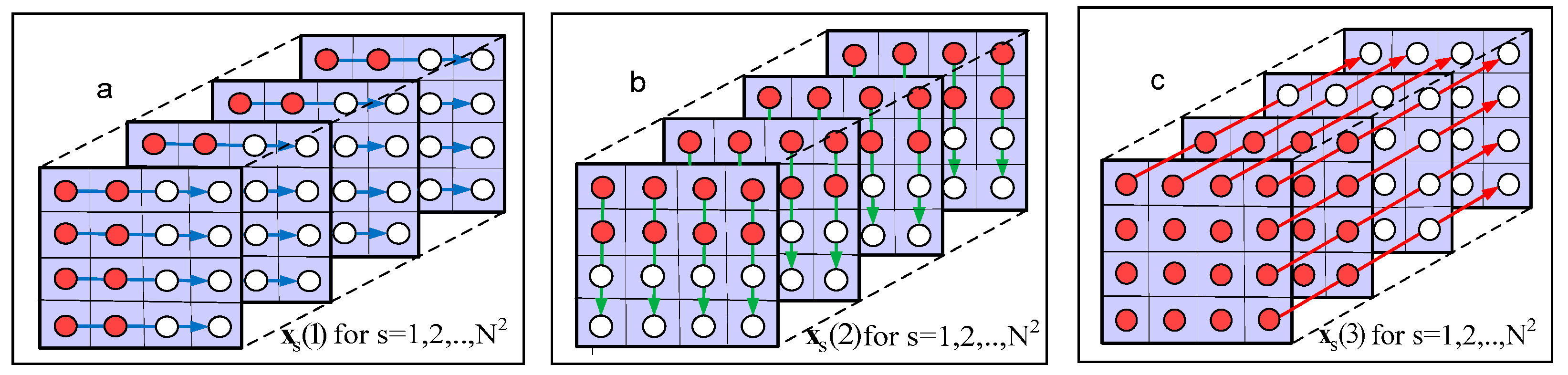
The choice of the orientation u = 1, 2, 3 of vectors $x_{\mathrm{s}}(\mathrm{u})$ in each stage S_u of 3D FO-AHKLT which ensures maximum decorrelation for the tensor $\mathbf{𝒳}$, is based on the relation between coefficients Δ(u), given in Table 1. Figure 3a–c shows the vectors $x_{\mathrm{s}}(1),$ $x_{\mathrm{s}}(2),$ $x_{\mathrm{s}}(3)$, which have horizontal, vertical and lateral orientation, correspondingly, and are obtained through unfolding mode u = 1, 2, 3 of the tensor $\mathbf{𝒳}$, of size 4 × 4 × 4. The couples of elements of the vectors $x_{\mathrm{q},\mathrm{s}}(\mathrm{u})$ for q = 1, 2 on which KLT_2×2 is applied in the lowest level of FO-HKLT, are colored in red and white.

Table 1. Adaptive choice of the orientation of vectors $x_{\mathrm{s}}(\mathrm{u})$ for u = 1, 2, 3, based on the correlation analysis.

No.	Relations for Δ(1), Δ(2), Δ(3)	Sequence of Stages Su in the 3D FO-AHKLT Execution (for u = 1, 2, 3)
1	Δ(1) > Δ(2) > Δ(3) Δ(1) = Δ(2) = Δ(3) Δ(1) > Δ(2) = Δ(3) Δ(1) = Δ(2) > Δ(3)	S1 → S2 → S3
2	Δ(1) > Δ(3) > Δ(2) Δ(1) > Δ(3) = Δ(2) Δ(1) = Δ(3) > Δ(2)	S1 → S3 → S2
3	Δ(2) > Δ(1) > Δ(3) Δ(2) > Δ(1) = Δ(3) Δ(2) = Δ(1) > Δ(3)	S2 → S1 → S3
4	Δ(2) > Δ(3) > Δ(1) Δ(2) > Δ(3) = Δ(1) Δ(2) = Δ(3) > Δ(1)	S2 → S3 → S1
5	Δ(3) > Δ(2) > Δ(1) Δ(3) > Δ(2) = Δ(1) Δ(3) = Δ(2) > Δ(1)	S3 → S2 → S1
6	Δ(3) > Δ(1) > Δ(2) Δ(3) > Δ(1) = Δ(2) Δ(3) = Δ(1) > Δ(2)	S3 → S1 → S2

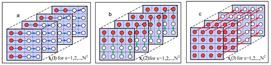
Figure 3. Orientations of vectors $x_{\mathrm{s}}(\mathrm{u})$ for u = 1, 2, 3 and N = 4 after unfolding mode u = 1, 2, 3 of the tensor $\mathbf{𝒳}$: (a) horizontal; (b) vertical; (c) lateral.

3.3. Evaluation of the Decorrelation Properties of FO-AHKLT

The qualities of the one-dimensional FO-AHKLT correspond to the decorrelation degree of the output eigen images, which defines the number of needed execution levels, n. As an example, here is given the evaluation of the decorrelation properties of the transform, for the case N = 8 and n = 3. In the hierarchical level p = 1, 2, 3 of FO-AHKLT, the covariance matrix $K_{\mathrm{y}}^{\mathrm{p}}$ of size 8 × 8, which represents the transformed 8-component vectors $y_{\mathrm{p},\mathrm{s}}(\mathrm{u})={[{\mathrm{y}}_{\mathrm{p},1,\mathrm{s}}(\mathrm{u}),{\mathrm{y}}_{\mathrm{p},2,\mathrm{s}}(\mathrm{u}),\dots ,{\mathrm{y}}_{\mathrm{p},8,\mathrm{s}}(\mathrm{u})]}^{\mathrm{T}}$, is:

$$K_{\mathrm{y}}^{\mathrm{p}}(\mathrm{u})=\mathrm{E}\{y_{\mathrm{p},\mathrm{s}}(\mathrm{u})·y_{\mathrm{p},\mathrm{s}}^{\mathrm{T}}(\mathrm{u})\}-\mathrm{E}\{y_{\mathrm{p},\mathrm{s}}(\mathrm{u})\}·\mathrm{E}{\{y_{\mathrm{p},\mathrm{s}}(\mathrm{u})\}}^{\mathrm{T}}=\left[\begin{array}{llll}{K}_{{\mathrm{y}}_1}^{\mathrm{p}}(\mathrm{u})& K_{{\mathrm{y}}_1,{\mathrm{y}}_2}^{\mathrm{p}}(\mathrm{u})& K_{{\mathrm{y}}_1,{\mathrm{y}}_3}^{\mathrm{p}}(\mathrm{u})& K_{{\mathrm{y}}_1,{\mathrm{y}}_4}^{\mathrm{p}}(\mathrm{u})\\ K_{{\mathrm{y}}_2,{\mathrm{y}}_1}^{\mathrm{p}}(\mathrm{u})& K_{{\mathrm{y}}_2}^{\mathrm{p}}(\mathrm{u})& K_{{\mathrm{y}}_2,{\mathrm{y}}_3}^{\mathrm{p}}(\mathrm{u})& K_{{\mathrm{y}}_2,{\mathrm{y}}_4}^{\mathrm{p}}(\mathrm{u})\\ K_{{\mathrm{y}}_3,{\mathrm{y}}_1}^{\mathrm{p}}(\mathrm{u})& K_{{\mathrm{y}}_3,{\mathrm{y}}_2}^{\mathrm{p}}(\mathrm{u})& K_{{\mathrm{y}}_3}^{\mathrm{p}}(\mathrm{u})& K_{\mathrm{y}3,{\mathrm{y}}_4}^{\mathrm{p}}(\mathrm{u})\\ K_{{\mathrm{y}}_4,{\mathrm{y}}_1}^{\mathrm{p}}(\mathrm{u})& K_{{\mathrm{y}}_4,{\mathrm{y}}_2}^{\mathrm{p}}(\mathrm{u})& K_{\mathrm{y}4,{\mathrm{y}}_3}^{\mathrm{p}}(\mathrm{u})& K_{{\mathrm{y}}_4}^{\mathrm{p}}(\mathrm{u})\end{array}\right]$$

(18)

for s = 1, 2, …, 64.

Here, the sub-matrices $K_{{\mathrm{y}}_{\mathrm{q}}}^{\mathrm{p}}(\mathrm{u})$ of size 2 × 2 (for q = 1, 2, 3, 4) are defined as:

$$K_{{\mathrm{y}}_{\mathrm{q}}}^{\mathrm{p}}(\mathrm{u})=\mathrm{E}\{y_{\mathrm{q},\mathrm{s}}^{\mathrm{p}}(\mathrm{u}),y_{\mathrm{q},\mathrm{s}}^{\mathrm{p} \mathrm{T}}(\mathrm{u})\}-\mathrm{E}\{y_{\mathrm{q},\mathrm{s}}^{\mathrm{p}}(\mathrm{u})\}·\mathrm{E}{\{y_{\mathrm{q},\mathrm{s}}^{\mathrm{p}}(\mathrm{u})\}}^{\mathrm{T}}=\left[\begin{array}{cc}{\lambda }_{1,\mathrm{q}}^{\mathrm{p}}(\mathrm{u})& 0\\ 0& {\lambda }_{2,\mathrm{q}}^{\mathrm{p}}(\mathrm{u})\end{array}\right]$$

(19)

These are the covariance matrices of the transformed vectors $y_{\mathrm{q},\mathrm{s}}^{\mathrm{p}}(\mathrm{u})={[{\mathrm{y}}_{\mathrm{q},1,\mathrm{s}}^{\mathrm{p}}(\mathrm{u}),{\mathrm{y}}_{\mathrm{q},2,\mathrm{s}}^{\mathrm{p}}(\mathrm{u})]}^{\mathrm{T}}$ in the group q for the level p, and ${\lambda }_{1,\mathrm{q}}^{\mathrm{p}}(\mathrm{u}),{\lambda }_{2,\mathrm{q}}^{\mathrm{p}}(\mathrm{u})$ are the eigen values of the covariance matrices $K_{{\mathrm{y}}_{\mathrm{q}}}^{\mathrm{p}}(\mathrm{u})$. Respectively,

$$K_{{\mathrm{y}}_{\mathrm{q}},{\mathrm{y}}_{\mathrm{k}}}^{\mathrm{p}}(\mathrm{u})=\mathrm{E}\{y_{\mathrm{q},\mathrm{s}}^{\mathrm{p}}(\mathrm{u})·y_{\mathrm{k},\mathrm{s}}^{\mathrm{p} \mathrm{T}}(\mathrm{u})\}-\mathrm{E}\{y_{\mathrm{q},\mathrm{s}}^{\mathrm{p}}(\mathrm{u})\}·\mathrm{E}{\{y_{\mathrm{k},\mathrm{s}}^{\mathrm{p}}(\mathrm{u})\}}^{\mathrm{T}} \mathrm{for} \mathrm{q},\mathrm{k}=1,2,3,4 (\mathrm{q}\ne \mathrm{k})$$

(20)

are the mutual covariance matrices of size 2 × 2 of the two-component vectors $y_{\mathrm{q},\mathrm{s}}^{\mathrm{p}}(\mathrm{u})$ and $y_{\mathrm{k},\mathrm{s}}^{\mathrm{p}} (\mathrm{u})$ for the couples of groups q and k from the level p.

After the rearrangement that follows the decomposition level p = 3, the vectors $y_{3,\mathrm{s}}(\mathrm{u})={[{\mathrm{y}}_{3,1,\mathrm{s}}(\mathrm{u}),{\mathrm{y}}_{3,2,\mathrm{s}}(\mathrm{u}),\dots ,{\mathrm{y}}_{3,8,\mathrm{s}}(\mathrm{u})]}^{\mathrm{T}}$ are transformed into vectors $e_{\mathrm{s}}(\mathrm{u})={[{\mathrm{e}}_{1,\mathrm{s}}(\mathrm{u}),{\mathrm{e}}_{2,\mathrm{s}}(\mathrm{u}),\dots ,{\mathrm{e}}_{8,\mathrm{s}}(\mathrm{u})]}^{\mathrm{T}}$. To evaluate the result of FO-AHKLT, the covariance matrix $K_{\mathrm{e}}^3(\mathrm{u})$ of the vectors $e_{\mathrm{s}} (\mathrm{u})$ is analyzed, from which the achieved decorrelation degree in the level is defined.

4. Adaptive Control for Each Level of FO-AHKLT

After the execution of FO-AHKLT in the current level p, from the transformed two-component vectors $y_{\mathrm{q},\mathrm{s}}^{\mathrm{p}}(\mathrm{u})={[{\mathrm{y}}_{\mathrm{q},1,\mathrm{s}}^{\mathrm{p}}(\mathrm{u}),{\mathrm{y}}_{\mathrm{q},2,\mathrm{s}}^{\mathrm{p}}(\mathrm{u})]}^{\mathrm{T}}$ for each group q = 1, 2, …, (N/2), through concatenation the N-dimensional vectors $y_{\mathrm{p},\mathrm{s}}(\mathrm{u})={[{\mathrm{y}}_{\mathrm{p},1,\mathrm{s}}(\mathrm{u}),{\mathrm{y}}_{\mathrm{p},2,\mathrm{s}}(\mathrm{u}),\dots ,{\mathrm{y}}_{\mathrm{p},\mathrm{n},\mathrm{s}}(\mathrm{u})]}^{\mathrm{T}}$ for p = 1, 2, …, n (n = lg₂N) and s = 1, 2, …, N² are obtained. At this moment, the decision to continue with the next level of FO-AHKLT, or to stop, must be taken. For this, the covariance matrix $K_{\mathrm{y}}^{\mathrm{p}}(\mathrm{u})$ of the vectors $y_{\mathrm{p},\mathrm{s}}(\mathrm{u})$ is analyzed for s = 1, 2, …, S, which defines the achieved decorrelation. In the case that the decorrelation is full, their matrix $K_{\mathrm{y}}^{\mathrm{p}}(\mathrm{u})$ is diagonal, and the algorithm is stopped. The proposed adaptive control of FO-AHKLT permits the process to stop earlier, despite that full decorrelation is not achieved, if the result is satisfactory. The decision to stop the FO-AHKLT in the current level p is defined by the relation:

$${\mathsf{\Lambda }}_{\mathrm{p}}={\displaystyle \sum _{\mathrm{i}=1}^{\mathrm{N}}{\displaystyle \sum _{\mathrm{j}=1}^{\mathrm{N}}{[{\mathrm{k}}_{{\mathrm{y}}_{\mathrm{p}},\mathrm{i},\mathrm{j}}(\mathrm{u})]}^2{}_{(\mathrm{i}\ne \mathrm{j})}}}\le {\delta }_1$$

(21)

Here, ${\mathrm{k}}_{{\mathrm{y}}_{\mathrm{p}},\mathrm{i},\mathrm{j}}(\mathrm{u})$ is the (i, j)th element of the matrix $K_{\mathrm{y}}^{\mathrm{p}}(\mathrm{u})$, and δ₁ is a threshold of small value, set in advance. In the case that the condition is satisfied, the calculations stop. Otherwise, the processing continues with the next FO-AHKLT level, p + 1. When the calculations for the second level are finished, the result is checked again, but in this case ${\mathrm{k}}_{{\mathrm{y}}_{\mathrm{p}+1},\mathrm{i},\mathrm{j}}(\mathrm{u})$ are the elements of the matrix $K_{\mathrm{y}}^{\mathrm{p}+1}(\mathrm{u})$ of the vectors $y_{\mathrm{p}+1,\mathrm{s}}(\mathrm{u})$, etc.

Taking into account the condition (21), the FO-AHKLT matrix defined in Equation (3) turns into:

$$T_{\mathrm{FO}-\mathrm{AHKLT}}(2^{\mathrm{n}})=\{\begin{array}{cc}{P}_{{\mathrm{p}}_0}{(2}^{\mathrm{}})[{\displaystyle \prod _{\mathrm{p}=1}^{{\mathrm{p}}_0}{G}_{\mathrm{p}}{(2}^{\mathrm{n}})}{] \mathrm{for} \mathrm{p}}_0<\mathrm{n}\hfill & \hfill \mathrm{if} {\mathsf{\Lambda }}_{{\mathrm{p}}_0}\le {\delta }_1;\\ P_{\mathrm{n}}{(2}^{\mathrm{n}})[{\displaystyle \prod _{\mathrm{p}=1}^{\mathrm{n}}{G}_{\mathrm{p}}{(2}^{\mathrm{n}})}] \mathrm{for} \mathrm{p}=1,2,\dots ,\mathrm{n}-1\hfill & \hfill \mathrm{if} {\mathsf{\Lambda }}_{\mathrm{p}}>{\delta }_1,\end{array}$$

(22)

$${\mathrm{y}}_{\mathrm{p},1,\mathrm{s}}^{\mathrm{q}}(\mathrm{u})=\{\begin{array}{cc}{\mathrm{y}}_{\mathrm{p}-1,1,\mathrm{s}}^{\mathrm{q}}(\mathrm{u}) {\cos \mathsf{\theta }}_{\mathrm{p},\mathrm{q}}(\mathrm{u})+{\mathrm{y}}_{\mathrm{p}-1,2,\mathrm{s}}^{\mathrm{q}}(\mathrm{u})\sin \mathsf{\theta }(\mathrm{u})\mathrm{p},\mathrm{q}\hfill & \hfill \mathrm{if} [{\mathrm{k}}_{\mathrm{p},3}^{\mathrm{q}}( \mathrm{u}){]}^2>{\delta }_2;\\ {\mathrm{y}}_{\mathrm{p}-1,1,\mathrm{s}}^{\mathrm{q}}(\mathrm{u}) \mathrm{if}\hfill & \hfill [{\mathrm{k}}_{\mathrm{p},3}^{\mathrm{q}}(\mathrm{u}){]}^2\le {\delta }_2,\end{array}$$

(23)

$${\mathrm{y}}_{\mathrm{p},2,\mathrm{s}}^{\mathrm{q}}(\mathrm{u})=\{\begin{array}{cc}{\mathrm{y}}_{\mathrm{p}-1,1,\mathrm{s}}^{\mathrm{q}}(\mathrm{u})\sin \mathsf{\theta }(\mathrm{u})\mathrm{p},\mathrm{q}-{\mathrm{y}}_{\mathrm{p}-1,2,\mathrm{s}}^{\mathrm{q}}(\mathrm{u})\cos \mathsf{\theta }(\mathrm{u})\mathrm{p},\mathrm{q}\hfill & \hfill \mathrm{if} [{\mathrm{k}}_{\mathrm{p},3}^{\mathrm{q}}(\mathrm{u}){]}^2>{\delta }_2;\\ {-\mathrm{y}}_{\mathrm{p}-1,2,\mathrm{s}}^{\mathrm{q}}(\mathrm{u}) \mathrm{if}\hfill & \hfill [{\mathrm{k}}_{\mathrm{p},3}^{\mathrm{q}}( \mathrm{u}){]}^2\le {\delta }_2\end{array}$$

(24)

for p = 2,3,…,n, q = 1, 2, …, (N/2) and ${\mathrm{k}}_{\mathrm{p},3}^{\mathrm{q}}(\mathrm{u})=\mathrm{E}\{{\mathrm{y}}_{\mathrm{p}-1,1,\mathrm{s}}^{\mathrm{q}}(\mathrm{u}),{\mathrm{y}}_{\mathrm{p}-1,2,\mathrm{s}}^{\mathrm{q}}(\mathrm{u})\}$.

For the level p = 1 only, the relations (22) and (23) are transformed as follows:

$${\mathrm{y}}_{1,1,\mathrm{s}}^{\mathrm{q}}(\mathrm{u})=\{\begin{array}{cc}{\mathrm{x}}_{1,1,\mathrm{s}}^{\mathrm{q}}(\mathrm{u}){\cos \mathsf{\theta }}_{1,\mathrm{q}}(\mathrm{u})+{\mathrm{x}}_{1,2,\mathrm{s}}^{\mathrm{q}}(\mathrm{u}) {\sin \mathsf{\theta }}_{1,\mathrm{q}}(\mathrm{u})\hfill & \hfill \mathrm{if} [{\mathrm{k}}_{1,3}^{\mathrm{q}}(\mathrm{u}){]}^2>{\delta }_2;\\ {\mathrm{x}}_{1,1,\mathrm{s}}^{\mathrm{q}}(\mathrm{u}) \mathrm{if}\hfill & \hfill [{\mathrm{k}}_{1,3}^{\mathrm{q}}(\mathrm{u}){]}^2\le {\delta }_2.\end{array}$$

(25)

$${\mathrm{y}}_{1,2,\mathrm{s}}^{\mathrm{q}}(\mathrm{u})=\{\begin{array}{cc}{\mathrm{x}}_{1,1,\mathrm{s}}^{\mathrm{q}}(\mathrm{u})\sin {\mathsf{\theta }}_{1,\mathrm{q}}(\mathrm{u})-{\mathrm{x}}_{1,2,\mathrm{s}}^{\mathrm{q}}(\mathrm{u})\cos {\mathsf{\theta }}_{1,\mathrm{q}}(\mathrm{u})\hfill & \hfill \mathrm{if} [{\mathrm{k}}_{1,3}^{\mathrm{q}}(\mathrm{u}){]}^2>{\delta }_2;\\ {-\mathrm{x}}_{1,2,\mathrm{s}}^{\mathrm{q}}(\mathrm{u}) \mathrm{if}\hfill & \hfill [{\mathrm{k}}_{1,3}^{\mathrm{q}}(\mathrm{u}){]}^2\le {\delta }_2,\end{array}$$

(26)

where ${[{\mathrm{k}}_{1,3}^{\mathrm{q}}(\mathrm{u})]}^2=\mathrm{E}\{{\mathrm{x}}_{1,1,\mathrm{s}}^{\mathrm{q}}(\mathrm{u}),{\mathrm{x}}_{1,2,\mathrm{s}}^{\mathrm{q}}(\mathrm{u})\}$.

In these relations, δ₂ is a threshold of small value, set in advance. The condition (21), together with the adaptive KLT_2×2 performed in accordance with relations (23)–(26), permits reducing the number of calculations without worsening the 3D FO-AHKLT decorrelation properties.

5. Algorithm 3D FO-AHKLT

On the basis of the 3D FO-HKLT tensor decomposition, together with the adaptive control of the directional vectorization on the input, the intermediate and the output tensor, and the correlation analysis, the algorithm called 3D FO-AHKLT is developed as Algorithm 1:

Algorithm1

Input: Third-order tensor $\mathbf{𝒳}$ of size N × N × N (N = 2n) with elements x(i, j, k), and threshold values, δ1, δ2;

The steps of the algorithm are given below:

1. Unfolding of the tensor $\mathbf{𝒳}$ (mode u = 1, 2, 3), thereby obtaining the corresponding groups of vectors, $x_{\mathrm{s}}(\mathrm{u})$.

2. Calculation of the covariance matrices $K_{\mathrm{y}}^{\mathrm{p}}(\mathrm{u})$ of the vectors $x_{\mathrm{s}}(\mathrm{u})$, for u = 1, 2, 3.

3. Calculation of the coefficients $\Delta (\mathrm{u})$ for u = 1, 2, 3, using the matrices $K_{\mathrm{y}}^{\mathrm{p}}(\mathrm{u})$.

4. Setting the sequence of stages Su1, Su2, Su3 for the execution of 3D FO-AHKLT, chosen in accordance with the relations between coefficients $\Delta (1), \Delta (2), \Delta (3)$.

5. Start of stage Su1, which comprises:

5.1. Execution of FO-AHKLT for the vectors $x_{\mathrm{s}}({\mathrm{u}}_1)$ with orientation u1 (for $\Delta ({\mathrm{u}}_1)=\max$), in correspondence with the calculation graph of n hierarchical levels and with a kernel—the adaptive KLT2×2, thereby obtaining the vectors $e_{\mathrm{s}}({\mathrm{u}}_1)$. In each level p = 1, 2, …, n is checked if the condition to stop the FO-AHKLT calculations is satisfied;

5.2. Folding of the tensor E of size N × N × N, by using the vectors $e_{\mathrm{s}}({\mathrm{u}}_1)$;

5.3. Unfolding of the tensor E (mode u2), thereby obtaining the vectors $x_{\mathrm{s}}({\mathrm{u}}_2)$ with orientation u2, for $\Delta ({\mathrm{u}}_2)\le \Delta ({\mathrm{u}}_1)$.

6. Start of stage Su2, which comprises:

6.1. Execution of FO-AHKLT for the vectors $x_{\mathrm{s}}({\mathrm{u}}_2)$ in correspondence with the computational graph of n hierarchical levels and with a kernel—the adaptive KLT2 × 2, thereby obtaining the vectors $y_{\mathrm{s}}({\mathrm{u}}_2)$. In each level p = 1, 2, …, n is checked if the condition to stop the FO-AHKLT calculations is satisfied;

6.2. Folding the tensor F of size N × N × N, by using the vectors $y_{\mathrm{s}}({\mathrm{u}}_2)$;

6.3. Unfolding the tensor F (mode u3), thereby obtaining the vectors $x_{\mathrm{s}}({\mathrm{u}}_3)$, with orientation u3, for $\Delta ({\mathrm{u}}_3)\le \Delta ({\mathrm{u}}_2)$;

7. Start of stage Su3, which comprises:

7.1. Execution of FO-AHKLT for the vectors $x_{\mathrm{s}}({\mathrm{u}}_3)$ in correspondence with the computational graph of n hierarchical levels and with a kernel—the adaptive KLT2 × 2, thereby obtaining the vectors $s_{\mathrm{s}}({\mathrm{u}}_3)$. In each level p = 1, 2, …, n is checked if the condition to stop the FO-AHKLT calculations is satisfied;

7.2. Folding of the tensor S of size N × N × N (N = 2n) by using the vectors $s_{\mathrm{s}}({\mathrm{u}}_3)$. The elements of the tensor S are the spectrum coefficients s (m, v, l).

8. Calculation of the transform matrices $T_{\mathrm{FO}-\mathrm{AHKLT}}^{\mathrm{t}}(2^{\mathrm{n}})$ for each stage t = 1, 2, 3 of the 3D FO-AHKLT in accordance with the relations below: $$e_{\mathrm{s}}({\mathrm{u}}_1)=T_{\mathrm{FO}-\mathrm{AHKLT}}^1{(2}^{\mathrm{n}})x_{\mathrm{s}}({\mathrm{u}}_1)\mathrm{for}\mathrm{s}=1, 2, \dots , {\mathrm{N}}^2;$$ (27) $$y_{\mathrm{s}}({\mathrm{u}}_2)=T_{\mathrm{FO}-\mathrm{AHKLT}}^2{(2}^{\mathrm{n}})x_{\mathrm{s}}({\mathrm{u}}_2)\mathrm{for}\mathrm{s}=1, 2, \dots , {\mathrm{N}}^2;$$ (28) $$s_{\mathrm{s}}({\mathrm{u}}_3)=T_{\mathrm{FO}-\mathrm{AHKLT}}^3{(2}^{\mathrm{n}})x_{\mathrm{s}}({\mathrm{u}}_3)\mathrm{for}\mathrm{s}=1, 2, \dots , {\mathrm{N}}^2.$$ (29)

9. Determination of the basic vectors $k_{\mathrm{m}}(1), k_{\mathrm{v}} (2), k_{\mathrm{l}}(3)$ for m, v, l = 0, 1, 2, …, N − 1, which are the rows of the matrices $T_{\mathrm{FO}-\mathrm{AHKLT}}^1{(2}^{\mathrm{n}}),T_{\mathrm{FO}-\mathrm{AHKLT}}^2{(2}^{\mathrm{n}}),T_{\mathrm{FO}-\mathrm{AHKLT}}^3{(2}^{\mathrm{n}})$. With this, the decomposition of the tensor $\mathbf{𝒳}$ in correspondence with Equation (1), is finished.

Output: Spectral tensor S, whose elements s(m, v, l) are the coefficients of the 3D FO-AHKLT.

As a result of the algorithm execution:

• The main part of the tensor energy is concentrated into a small number of coefficients s(m, v, l) of the spectrum tensor S, for m, v, l = 0, 1, 2;
• The decomposition components of the tensor are uncorrelated.

6. Comparative Evaluation of the Computational Complexity

For the computation of the covariance matrix $K_{\mathrm{y}}^{\mathrm{p}}(\mathrm{u})=\mathrm{E}\{y_{\mathrm{p},\mathrm{s}}(\mathrm{u})·y_{\mathrm{p},\mathrm{s}}^{\mathrm{T}}(\mathrm{u})\}-\mathrm{E}\{y_{\mathrm{p},\mathrm{s}}(\mathrm{u})\}·\mathrm{E}{\{y_{\mathrm{p},\mathrm{s}}(\mathrm{u})\}}^{\mathrm{T}}$ of size N × N for N = 2ⁿ, in correspondence with Equation (17), ${\mathrm{A}}_{K_{\mathrm{y}}^{\mathrm{p}}}(\mathrm{n})=3\times 2^{2\mathrm{n}}$ additions and ${\mathrm{M}}_{K_{\mathrm{y}}^{\mathrm{p}}}(\mathrm{n})=2^{2\mathrm{n}}$ multiplications are needed. Then, the total number of the operations needed for the calculation of $K_{\mathrm{y}}^{\mathrm{p}}(\mathrm{u})$ is:

$${\mathrm{O}}_{K_{\mathrm{y}}^{\mathrm{p}}}(\mathrm{n})={\mathrm{A}}_{K_{\mathrm{y}}^{\mathrm{p}}}(\mathrm{n})+{\mathrm{M}}_{K_{\mathrm{y}}^{\mathrm{p}}}(\mathrm{n})=4\times 2^{2\mathrm{n}} \mathrm{for} \mathrm{p}=1, 2, \dots , \mathrm{n}$$

(30)

For the n levels of the algorithm FO-HKLT is obtained:

$${\displaystyle \sum _{\mathrm{p}=1}^{\mathrm{n}}{\mathrm{O}}_{K_{\mathrm{y}}^{\mathrm{p}}}(\mathrm{n})}=4\times 2^{2\mathrm{n}}\mathrm{n}$$

(31)

For the calculation of Δ_u(u) in correspondence with Equation (17), ${\mathrm{A}}_{\Delta }{}_{\mathrm{u}}(\mathrm{n})=2^{2\mathrm{n}}-1$ additions and ${\mathrm{M}}_{{\Delta }_{\mathrm{u}}}(\mathrm{n})=2^{2\mathrm{n}}+1$ multiplications are needed. Then,

$${\mathrm{O}}_{{\Delta }_{\mathrm{u}}}(\mathrm{n})={\mathrm{A}}_{{\Delta }_{\mathrm{u}}}(\mathrm{n})+{\mathrm{M}}_{{\Delta }_{\mathrm{u}}}(\mathrm{n})=2\times 2^{2\mathrm{n}} \mathrm{for} \mathrm{u}=1, 2, 3$$

(32)

Hence,

$${\displaystyle \sum _{\mathrm{u}=1}^3{\mathrm{O}}_{{\Delta }_{\mathrm{u}}}(\mathrm{n})}=6\times 2^{2\mathrm{n}}.$$

(33)

In accordance with [17], the computational complexity (or Complexity) of FO-HKLT is defined by taking into account the number of needed additions ${\mathrm{A}}_{\mathrm{HKLT}}^{\mathrm{FO}}(\mathrm{n})=2^{\mathrm{n}-1}(5\times 2^{2\mathrm{n}}+1)\mathrm{n}\approx 2.5\times 2^{3\mathrm{n}}\mathrm{n}$, and multiplications ${\mathrm{M}}_{\mathrm{HKLT}}^{\mathrm{FO}}(\mathrm{n})=2^{\mathrm{n}-1}(7\times 2^{2\mathrm{n}}+5)\mathrm{n}\approx 3.5\times 2^{3\mathrm{n}}\mathrm{n}.$ Hence, the total number of operations needed for the 3D FO-HKLT execution is:

$${\mathrm{O}}_{\mathrm{HKLT}}^{3\mathrm{DFO}}(\mathrm{n})={\mathrm{A}}_{\mathrm{HKLT}}^{3\mathrm{DFO}}(\mathrm{n})+{\mathrm{M}}_{\mathrm{HKLT}}^{3\mathrm{DFO}}(\mathrm{n})\approx 18\times 2^{3\mathrm{n}}\mathrm{n}$$

(34)

The total number of operations needed for the execution of the algorithm 3D FO-AHKLT (without taking into consideration the possibility to stop the processing earlier than the last level) is:

$${\mathrm{O}}_{\mathrm{AHKLT}}^{3\mathrm{DFO}}(\mathrm{n})={\mathrm{A}}_{\mathrm{AHKLT}}^{3\mathrm{DFO}}(\mathrm{n})+{\mathrm{M}}_{\mathrm{AHKLT}}^{3\mathrm{DFO}}(\mathrm{n})\approx 2^{2\mathrm{n}+1}[2\mathrm{n}(9\times 2^{\mathrm{n}-1}+1)+3]$$

(35)

For the H-Tucker and TT decomposition of a cubical tensor of size N = 2ⁿ, in accordance with [17], the number of needed operations is:

$${\mathrm{O}}_{\mathrm{HT}}(\mathrm{n})=2^{3\mathrm{n}}(2^{\mathrm{n}+1}+3), {\mathrm{O}}_{\mathrm{TT}}(\mathrm{n})=3\times 2^{4\mathrm{n}}$$

(36)

Compared to H-Tucker and TT, the Complexity of the new decomposition decreases together with the growth of n. In the general case, the relative Complexity of 3D FO-AHKLT with respect to decompositions H-Tucker and TT is evaluated in accordance with the relations below:

$${\mathsf{\psi }}_1(\mathrm{n})=\frac{{\mathrm{O}}_{\mathrm{HT}}(\mathrm{n})}{{\mathrm{O}}_{\mathrm{AHKLT}}^{3\mathrm{DFO}}(\mathrm{n})}=2^{\mathrm{n}-1}\frac{2^{\mathrm{n}+1}+3}{2\mathrm{n}(9\times 2^{\mathrm{n}-1}+1)+3}$$

(37)

$${\mathsf{\psi }}_2(\mathrm{n})=\frac{{\mathrm{O}}_{\mathrm{TT}}(\mathrm{n})}{{\mathrm{O}}_{\mathrm{AHKLT}}^{3\mathrm{DFO}}(\mathrm{n})}=2^{2\mathrm{n}-1}\frac{3}{2\mathrm{n}(9\times 2^{\mathrm{n}-1}+1)+3}$$

(38)

For example, for n = 8 the results are: ${\mathsf{\psi }}_1(8)=3.57$ and ${\mathsf{\psi }}_2(8)=5.33$.

For the case when the new decomposition must have minimum Complexity, the transform kernel KLT_2×2 could be replaced by WHT of the same size (2 × 2), which in correspondence with Equation (10), is the particular case of KLT_2×2 for the fixed value of ${\mathsf{\theta }}_{1,2}=\mathsf{\pi }/4$. According to [19], the Complexity of the 3D Fast Walsh-Hadamard Transform (3D-FWHT) evaluated through the total number of operations ${\mathrm{O}}_{3\mathrm{D}-\mathrm{FWHT}}(\mathrm{n})$ is defined by the relation:

$${\mathrm{O}}_{3\mathrm{D}-\mathrm{FWHT}}(\mathrm{n})={\mathrm{A}}_{3\mathrm{D}-\mathrm{FWHT}}(\mathrm{n})+{\mathrm{M}}_{3\mathrm{D}-\mathrm{FWHT}}(\mathrm{n})=3\times 2^{3\mathrm{n}}\mathrm{n}$$

(39)

Then, for the Complexity of 3D-FWHT with ADV (3D-AFWHT), we obtain:

$${\mathrm{O}}_{3\mathrm{D}-\mathrm{AFWHT}}(\mathrm{n})={\mathrm{A}}_{3\mathrm{D}-\mathrm{AFWHT}}(\mathrm{n})+{\mathrm{M}}_{3\mathrm{D}-\mathrm{AFWHT}}(\mathrm{n})\approx 2^{2\mathrm{n}}[3\times 2^{\mathrm{n}}\mathrm{n}+2(2\mathrm{n}+3)]$$

(40)

The relative Complexity of 3D FO-AHKLT with respect to 3D-AFWHT is defined by the relation:

$${\mathsf{\psi }}_3(\mathrm{n})=\frac{{\mathrm{O}}_{\mathrm{AHKLT}}^{3\mathrm{DFO}}(\mathrm{n})}{{\mathrm{O}}_{3\mathrm{D}-\mathrm{AFWHT}}(\mathrm{n})}=2\frac{2\mathrm{n}(9\times 2^{\mathrm{n}-1}+1)+3}{3\times 2^{\mathrm{n}}\mathrm{n}+2(2\mathrm{n}+3)}$$

(41)

Hence, for the example value n = 8, it is ${\mathsf{\psi }}_3(\mathrm{n})=5.97$, and the relative Complexities of H-Tucker and TT vs. 3D-AFWHT are ${\mathrm{O}}_{\mathrm{H}\mathrm{T}}(8)/{\mathrm{O}}_{3\mathrm{D}-\mathrm{AFWHT}}(8)=21.33$ and ${\mathrm{O}}_{\mathrm{TT}}(8)/{\mathrm{O}}_{3\mathrm{D}-\mathrm{AFWHT}}(8)=31.84$, correspondingly.

In Table 2 are given the values of coefficients ${\mathsf{\psi }}_1(\mathrm{n})$, ${\mathsf{\psi }}_2(\mathrm{n})$ and ${\mathsf{\psi }}_3(\mathrm{n})$, calculated in accordance with Equations (36), (37) and (40), for n = 2, 3, …, 10. From the table, it is seen that for n > 5, the values of coefficients ${\mathsf{\psi }}_1(\mathrm{n})$ and ${\mathsf{\psi }}_2(\mathrm{n})$ are higher than “1” and grow fast together with n, while for the same values of n, the coefficient ${\mathsf{\psi }}_3(\mathrm{n})$ increases a little in the range from 4 up to 6.

Table 2. Relative Complexity of H-Tucker and TT vs. 3D FO-AHKLT and of 3D FO-AHKLT vs. 3D-AFWHT.

n	2	3	4	5	6	7	8	9	10
${\mathsf{\psi }}_1(\mathrm{n})$	0.28	0.34	0.48	0.74	1.21	2.05	3.57	6.34	11.39
${\mathsf{\psi }}_2(\mathrm{n})$	0.30	0.42	0.66	1.06	1.77	3.04	5.33	9.47	17.06
${\mathsf{\psi }}_3(\mathrm{n})$	4.16	5.00	5.46	5.74	5.87	5.94	5.97	5.98	5.99

From the comparison follow the conclusions below:

• The new hierarchical decomposition has low Complexity, which decreases together with the growth of n faster than those of the H-Tucker and TT decompositions;
• Significant reduction in the decomposition Complexity could be achieved through replacement of the kernel KLT_2×2 by WHT_2×2. In this particular case, the decrease in the decomposition Complexity results in a lower decorrelation degree;
• For the case n = 8, the Complexity of the algorithm 3D-AFWHT is approximately 6 times lower than that of the 3D FO-AHKLT;
• The Complexity of algorithms 3D FO-AHKLT and 3D-AFWHT was evaluated without taking into consideration the use of the adaptive KLT_2×2 and the possibility to stop the execution prior to the maximum level n. Equations (35) and (40) give the maximum values of Complexity used for the evaluation of the compared algorithms.

7. Conclusions

This work presented the new algorithm 3D FO-AHKLT, aimed at the decorrelation of the elements of a cubical tensor of size N = 2ⁿ. The Complexity of the algorithm was evaluated and compared with that of other, similar algorithms, and its efficiency was shown. The main qualities of the tensor decomposition 3D FO-AHKLT are:

• Efficient decorrelation of the calculated components;
• Concentration of the tensor energy into a small number of decomposition components;
• Lack of iterations;
• Low Complexity;
• The capacity for parallel recursive implementation, which reduces the needed memory volume;
• The capacity for additional significant Complexity reduction through the use of the algorithm 3D-AFWHT, depending on the needs of the implemented application.

The presented algorithms 3D FO-AHKLT and 3D-AFWHT could be generalized for tensors with three different dimensions $2^{{\mathrm{n}}_1}\times 2^{{\mathrm{n}}_2}\times 2^{{\mathrm{n}}_3}$ (i.e., for ${\mathrm{n}}_1\ne {\mathrm{n}}_2\ne {\mathrm{n}}_3$). The choice of the offered hierarchical 3D decompositions depends on the requirements and limitations of their Complexity imposed by the application area.

The future investigations of 3D FO-AHKLT and 3D-AFWHT will be aimed at the evaluation of their characteristics compared to famous tensor decompositions, in order to define the best settings and to define the most efficient applications for tensor image compression, feature space reduction, filtration, analysis, search and recognition of multidimensional visual information, deep learning, etc. The future development of the presented algorithm will be aimed at applications related to tree tensor network [20], multiway array (tensor) data analysis [21,22], tensor decompositions in neural networks for tree-structured data, etc.

References

- Liu, Y.; Liu, J.; Long, Z.; Zhu, C. Tensor Decomposition. In Tensor Computation for Data Analysis; Springer: Cham, Switzerland, 2021; pp. 19–57. [Google Scholar]
- Ji, Y.; Wang, Q.; Li, X.; Liu, J. A Survey on Tensor Techniques and Applications in Machine Learning. IEEE Access 2019, 7, 162950–162990. [Google Scholar] [CrossRef]
- Cichocki, A.; Mandic, D.; Phan, A.; Caiafa, C.; Zhou, G.; Zhao, Q.; De Lathauwer, L. Tensor Decompositions for Signal Processing Applications: From Two-Way to Multiway Component Analysis. IEEE Signal Process. Mag. 2015, 32, 145–163. [Google Scholar] [CrossRef] [Green Version]
- Sidiropoulos, N.; De Lathauwer, L.; Fu, X.; Huang, K.; Papalexakis, E.; Faloutsos, C. Tensor Decomposition for Signal Processing and Machine Learning. IEEE Trans. Signal Proc. 2017, 65, 3551–3582. [Google Scholar] [CrossRef]
- Oseledets, I. Tensor-train decomposition. Siam J. Sci. Comput. 2011, 33, 2295–2317. [Google Scholar] [CrossRef]
- Grasedyck, L. Hierarchical Singular Value Decomposition of Tensors. Siam J. Matrix Anal. Appl. 2010, 31, 2029–2054. [Google Scholar] [CrossRef] [Green Version]
- Ozdemir, A.; Zare, A.; Iwen, M.; Aviyente, S. Extension of PCA to Higher Order Data Structures: An Introduction to Tensors, Tensor Decompositions, and Tensor PCA. Proc. IEEE 2018, 106, 1341–1358. [Google Scholar]
- Vasilescu, M.; Kim, E. Compositional Hierarchical Tensor Factorization: Representing Hierarchical Intrinsic and Extrinsic Causal Factors. In Proceedings of the 25th ACM SIGKDD Conference on Knowledge Discovery and Data Mining (KDD): Tensor Methods for Emerging Data Science Challenges, Anchorage, NY, USA, 2–4 August 2019; p. 9. [Google Scholar]
- Wang, P.; Lu, C. Tensor Decomposition via Simultaneous Power Iteration. In Proceedings of the 34th International Conference on Machine Learning (PMLR), Sydney, Australia, 6–9 August 2017; Volume 70, pp. 3665–3673. [Google Scholar]
- Ishteva, M.; Absil, P.; Van Dooken, P. Jacoby Algorithm for the Best Low Multi-linear Rank Approximation of Symmetric Tensors. SIAM J. Matrix Anal. Appl. 2013, 34, 651–672. [Google Scholar] [CrossRef]
- Zniyed, Y.; Boyer, R.; Almeida, A.; Favier, G. A TT-based Hierarchical Framework for Decomposing High-Order Tensors. SIAM J. Sci. Comput. 2020, 42, A822–A848. [Google Scholar] [CrossRef] [Green Version]
- Kernfeld, E.; Kilmer, M.; Aeron, S. Tensor–tensor products with invertible linear transforms. Linear Algebra Appl. 2015, 485, 545–570. [Google Scholar]
- Keegany, K.; Vishwanathz, T.; Xu, Y. A Tensor SVD-based Classification Algorithm Applied to fMRI Data. arXiv 2021, arXiv:2111.00587v1. [Google Scholar]
- Rao, K.; Kim, D.; Hwang, J. Fast Fourier Transform: Algorithms and Applications; Springer: Dordrecht, The Netherlands, 2010; pp. 166–170. [Google Scholar]
- Ahmed, N.; Rao, K. Orthogonal Transforms for Digital Signal Processing; Springer: Berlin/Heidelberg, Germany, 1975; pp. 86–91. [Google Scholar]
- Kountchev, R.; Kountcheva, R. Adaptive Hierarchical KL-based Transform: Algorithms and Applications. In Computer Vision in Advanced Control Systems: Mathematical Theory; Favorskaya, M., Jain, L., Eds.; Springer: Berlin/Heidelberg, Germany, 2015; Volume 1, pp. 91–136. [Google Scholar]
- Kountchev, R.; Mironov, R.; Kountcheva, R. Complexity Estimation of Cubical Tensor Represented through 3D Frequency-Ordered Hierarchical KLT. Symmetry 2020, 12, 1605. [Google Scholar] [CrossRef]
- Lu, H.; Kpalma, K.; Ronsin, J. Motion descriptors for micro-expression recognition. In Signal Processing: Image Communication; Elsevier: Amsterdam, The Netherlands, 2018; Volume 67, pp. 108–117. [Google Scholar]
- Kountchev, R.; Mironov, R.; Kountcheva, R. Hierarchical Cubical Tensor Decomposition through Low Complexity Orthogonal Transforms. Symmetry 2020, 12, 864. [Google Scholar] [CrossRef]
- Cichocki, A.; Phan, H.; Zhao, Q.; Lee, N.; Oseledets, I.; Sugiyama, M.; Mandic, D. Tensor networks for dimensionality reduction and large-scale optimizations: Part 2 Applications and future perspectives. Found. Trends Mach. Learn. 2017, 9, 431–673. [Google Scholar] [CrossRef]
- Abhyankar, S.S.; Christensen, C.; Sundaram, G.; Sathaye, A.M. Algebra, Arithmetic and Geometry with Applications: Papers from Shreeram S. Abhyankar's 70th Birthday Conference; Springer Science & Business Media: Berlin/Heidelberg, Germany, 2004; pp. 457–472. [Google Scholar]
- Peters, J. Computational Geometry, Topology and Physics of Digital Images with Applications: Shape Complexes, Optical Vortex Nerves and Proximities; Springer Nature: Cham, Switzerland, 2019; pp. 1–115. [Google Scholar]
Publisher’s Note: MDPI stays neutral with regard to jurisdictional claims in published maps and institutional affiliations. |
© 2022 by the authors. Licensee MDPI, Basel, Switzerland. This article is an open access article distributed under the terms and conditions of the Creative Commons Attribution (CC BY) license (https://creativecommons.org/licenses/by/4.0/).