A Deep Learning-Based Intelligent Garbage Detection System Using an Unmanned Aerial Vehicle

Abstract

A population explosion has resulted in garbage generation on a large scale. The process of proper and automatic garbage collection is a challenging and tedious task for developing countries. This paper proposes a deep learning-based intelligent garbage detection system using an Unmanned Aerial Vehicle (UAV). The main aim of this paper is to provide a low-cost, accurate and easy-to-use solution for handling the garbage effectively. It also helps municipal corporations to detect the garbage areas in remote locations automatically. This automation was derived using two Convolutional Neural Network (CNN) models and images of solid waste were captured by the drone. Both models were trained on the collected image dataset at different learning rates, optimizers and epochs. This research uses symmetry during the sampling of garbage images. Homogeneity regarding resizing of images is generated due to the application of symmetry to extract their characteristics. The performance of two CNN models was evaluated with the state-of-the-art models using different performance evaluation metrics such as precision, recall, F1-score, and accuracy. The CNN1 model achieved better performance for automatic solid waste detection with 94% accuracy.

1. Introduction

Waste implies any unused materials and is rejected as worthless. Waste (also known as rubbish, trash, refuse, garbage, junk) can be unwanted or useless materials. Each and every country generates millions of tons of waste every year and this is rapidly increasing every year. For example, America, a developed nation, generates 2 kg of municipal solid garbage per day per person, which contributes to 55% of residential waste. In addition, developing countries produce 50% of biodegradable waste and the waste generated by the human can be witnessed across the globe. For instance, mountains have thousands of pounds of garbage accumulated due to littering and cleaning this garbage in such areas can be tricky.

Waste management is now becoming a challenging issue for many waste management organizations. As per the current scenario, the amount of city waste is increasing but its disposal and management capacity is declining. Therefore, it becomes difficult to dispose of this waste in an efficient and timely manner [1]. The population is also increasing astoundingly in big cities, which leads to an increase in the production of goods, which ends in the generation of a huge amount of solid waste. The collection, management and storage of this waste requires great effort as it has an adverse effect on the environment as well as public health. Solid waste in cities can choke the water drainage systems leading to floods and other disastrous concerns. Thus, waste detection and management mechanisms are required nowadays to evade such crises. At present, there has not been any public records regarding process of waste detection and management. Therefore, accurately detecting and classifying several types of garbage is important to improve quality of life and the environment. In recent years, due to expansion of deep learning, convolution neural networks have been applied in garbage detection. The government and waste management organizations can use UAV technology for managing waste efficiently. UAVs can simplify many operations in waste management such as garbage collection or landfill monitoring [2].

In recent years, UAVs are becoming effective low-cost image-capturing platforms for monitoring environments with high accuracy [3]. The UAV can identify litterbugs and collect litter garbage at public areas like parks and beaches. A CNN-based model is used to train several images captured from clean and polluted areas. Deep CNN has recently been used in image classification tasks such as automatic classification, object detection and semantic segmentation [4]. The process of validating and testing the preprocessed images has been explored to hills and coastal tourism applications through probabilities of classifying images and predicting clean shores and hill areas [5]. The images of the sampled material are taken at different time intervals between dusk and dawn in ambient light including visible light, ultraviolet light, and mixed visible and ultraviolet light. The best classification result was obtained on the sample material images shot under mixed visible and ultraviolet light [6]. In the image processing technique, the waste identification and classification must be based upon the transfer learning and convolution neural network [7], whereas the Support Vector Machine (SVM) is used to identify many types of garbage [8].

There is a long-felt need to have an automated analyzing technique to make the right decisions. These automated techniques can help waste management organizations handle the garbage efficiently based on the application of symmetry. Symmetry creates balance that is required in all spheres of life. In this contemporary period, deep learning is used for image retrieval and it is a significant issue to retrieve appropriate pictures with preciseness, which nonetheless neglects the symmetry for feature extraction. There are some research questions regarding this work:

RQ.1: What techniques have been used for garbage detection?

RQ.2: What kind of data or dataset have been used to carry out this process?

RQ.3: What are the different performance measures used in this work?

This paper aims to provide a low-cost, fast, accurate and easy-to-use solution for government and waste management organizations to handle the garbage effectively inspired by the symmetry theory. In this article, the major contribution of the author is as follows:

• A dataset is prepared that contains several images from the garbage area as well as the clean area which is captured using a UAV in different regions.
• Next, a CNN-based model is proposed in this paper that is simulated on the collected image dataset which helps in automatic waste management.
• The overall performance of this proposed model was evaluated in comparison with the state of art models.

The rest of the paper follows this sequence: Section 2 presents an image dataset of solid waste captured using a UAV. Applying augmentation enabled the class distribution of the dataset to achieve better accuracy. Next, Section 3 illustrates a new proposed CNN-based model that detects solid waste using a prepared dataset. Section 4 compares the proposed model with other state-of-the-art models. Finally, Section 5 concludes the paper.

2. Related Works

Vo et al. [9] used the CNN technique to extract the features from the image dataset and ridge regression was used to combine the two models’ image feature datasets. Ruiz et al. [10] used SVM as a classifier in the designed model and VN-trash dataset was used to train the CNN model, which contains images. The VN-trash dataset was categorized into different categories. The pre-trained model already existed and can also be used to categorize different types of solid waste materials. The comparative analysis of the performance of the Resnet and the inception module on the trash net dataset had shown 88.6% accuracy achieved by the inception module. Bobulski et al. [11] proved that plastic waste is a big menace and CNN-based models played a vital role in detecting different types of plastic categories. Gyawali et al. [12] focused on pre-trained models like Vgg-16, ResNet-50 and ResNet18. The ResNet-18 achieved a validation accuracy of 87.8% on the dataset. Several kinds of research on automatic garbage collection had been conducted in the past. Merely garbage collection and disposal was not enough. Garbage collection has to be substantiated by a proper recycling system. Gupta et al. [13] sorted the garbage into metals, plastic, glass, paper, etc., enabling efficient recycling and reuse. Huiyu et al. [14] applied machine learning and artificial intelligence for proper waste management, which yielded 67% accuracy. A data set of 600 images were divided into five categories containing 120 images each. The learning rate, train/test image, epoch, and batch size were used as CNN parameters. The recognition rate obtained was 83.35%. Chu et al. [15] compared the Multilayer Hybrid System (MHS) and CNN system on a single dataset. The data set was divided into six categories: paper, metal, glass, fruits, plastic, etc., and the MHS system achieved an accuracy rate above 90%. In another study by Costa et al. [16], solid waste was classified into four categories: glass, paper, plastic and metal, where using the SVM and VGG-16 as pre-trained models yielded an accuracy of 93%. Zhao et al. [17] used UAV RGB and multispectral images to extract rice lodging with dice coefficients of 0.94 and 0.92, respectively, which was based on U-Net architecture. Soundarya et al. [18] captured, identified, and segregated images of single waste into biodegradable and non-biodegradable waste using Raspberry Pi. Likewise, Yi et al. [19] used very high-resolution aerial images to map urban buildings using DeepResUNet with a 0.93 F1 score and high accuracy. Ahmad et al. [20] proposed a double fusion scheme that combined two deep learning models. The technique improved the performance of the system. Altikat et al. [21] used a dataset of 2527 images that were divided into six different categories. Deep learning was applied to classify plastic, glass, organic waste and paper, where 70% accuracy was achieved by five-layer architecture and 61.67% accuracy was achieved by four-layer architecture. Seredkin et al. [22] trained a model on approximately 13,000 solid waste images and achieved an accuracy of 64%. The solid waste was shifted onto the conveyer belt and the CNN-based model sorted the solid waste into three classified categories: metal can, polythene and plastic bottle.

Wang et al. [23] used a CNN model to identify and classify recyclable objects. Resnet-50 CNN was pre-trained to extract features and the TrashNet dataset was trained for classification. The proposed model achieved a 48.4% detection rate and 92.4% accuracy. Zhang et al. [24] designed a deep learning-based solid waste sorting robot that sorted the solid waste moving on a conveyer belt using a depth camera. The waste was classified into plastic, metal and bottle. Another CNN-based solution given by Brintha et al. [25] classified waste into glass, plastic, wood, textile and cardboard. Mudita et al. [26] defined fault tolerance as a major concern to ensure the reliability dependability and availability of critical systems. Therefore, the faults should be predicted before their occurrence to lessen failure impact. Moreira et al. [27] reviewed various mobile apps to analyze the posture of individuals and highlighted their advantages. Uppal et al. [28] designed a prototype of an IoT-based office that controls devices at the workplace and predicts devices needing repair or replacement. This reduces the burden on the worker and helps out in improving the mental and physical health of employees. Singh et al. [29] proposed an architecture based on CNN for identifying the names of months in the Gurumukhi language. Uppal et al. [30] presented a novel technique anointed as a fall curve to distinguish faults in sensors. Malik et al. [31] presented a framework to balance the load of fog nodes that manage the needs of smart real-time applications. Garcia-Garin et al. [32] designed a deep learning model that detects floating marine waste in aerial images. The model was trained on 3700 pictures that were taken during aircraft and drone surveys. An accuracy of 0.81 was considered the best, which was calculated during cross-validation. This model was implemented in an application based on the “Shiny” package. Sliusar et al. [33] did a comprehensive review on municipal solid waste management and landfilling via drone technology. The issues and promising areas of further research are also discussed in this paper.

3. Materials and Methods

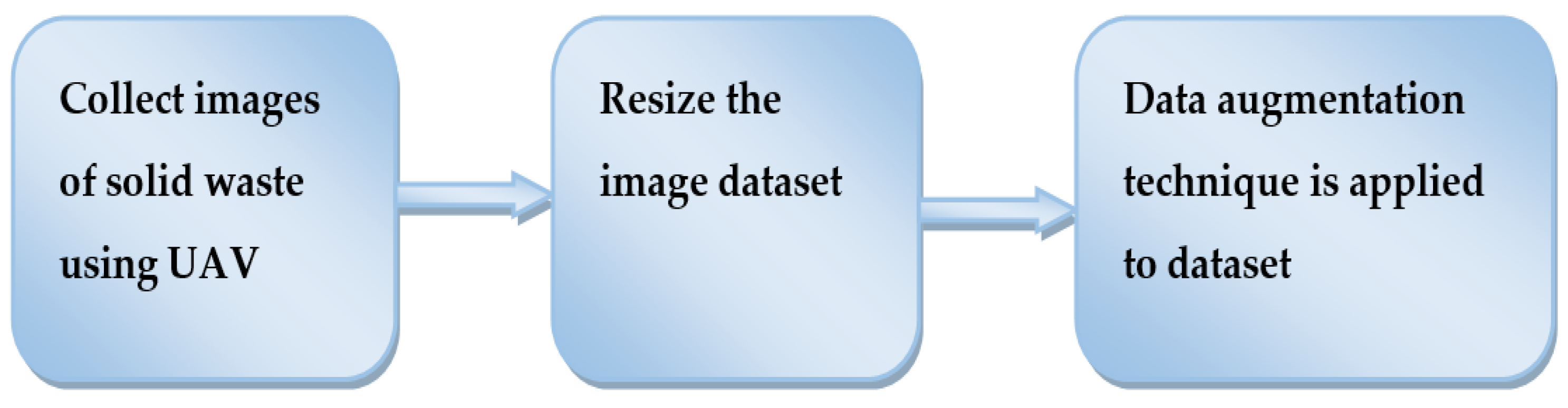
Garbage detection and collection in hilly and coastal areas is a challenging task. Therefore, a CNN-based solid waste detection system using a UAV is proposed for such purposes. The image dataset contains images of plastic waste, agricultural waste, biomedical waste, construction waste, household waste, and electronic waste. Figure 1 shows the flow diagram of the dataset preprocessing.

Figure 1. Flow diagram of dataset preprocessing.

3.1. Capturing Images Using UAV

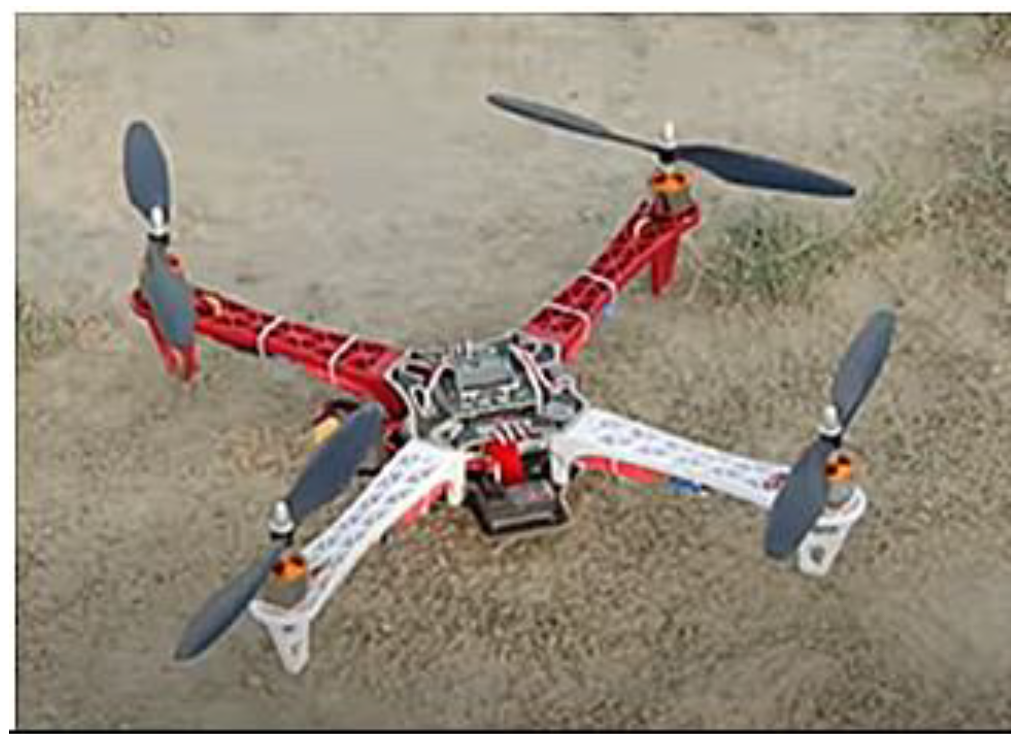
Dataset collection is a considerable challenge in deep learning. The proposed system used a quadcopter with an 8 MP camera (Figure 2) to capture the images of waste areas. There were some places where capturing an image was difficult for the UAV. At such places, the drone recorded a video clip, which was further converted into different image frames.

Figure 2. Drone Used to Capture Solid Waste.

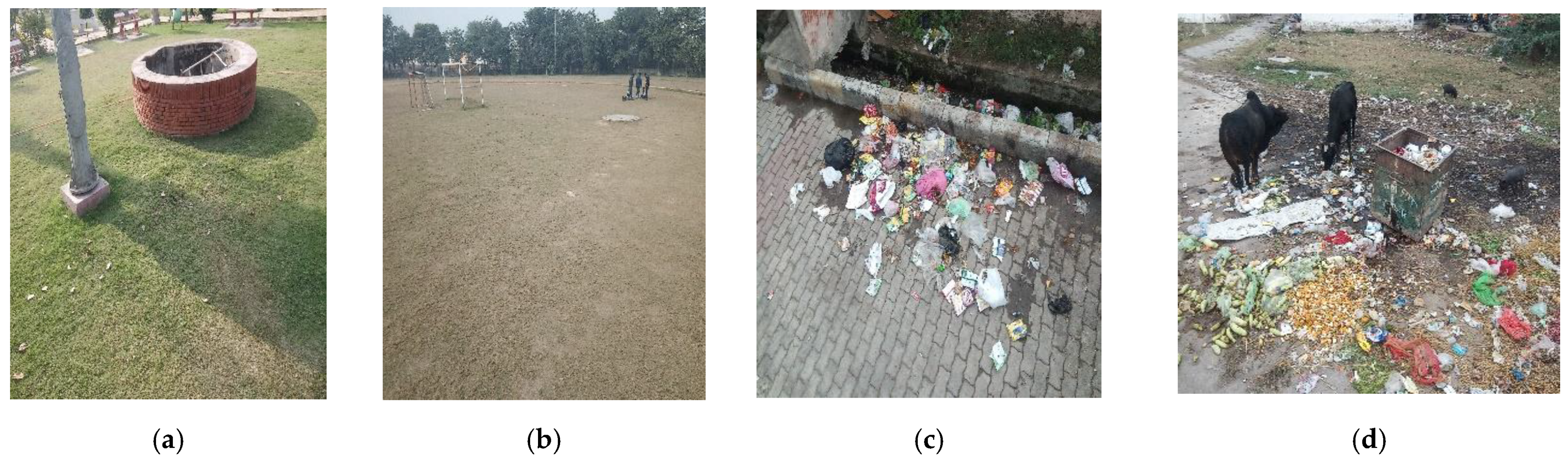
Initially, 2000 images were captured at various time intervals from dusk to dawn. Out of these 2000 images, 1000 images were of clean areas and 1000 images were of garbage areas. The images were captured using a UAV with an 8 MP camera whose height was kept a maximum of 10 feet from ground level. Figure 3 shows the dataset images of a clean area and solid waste area.

Figure 3. UAV Image Dataset: (a) Clean Area-1, (b) Clean Area-2 (c) Solid Waste -1, (d) Solid Waste-2.

3.2. Image Resizing

The dataset of images was collected from different regions of the Punjab state of India located in Asia. The size of the images captured from the UAV was initially 1080 × 1920 pixels, but were resized further to 224 × 224 pixels. Some images were collected from the internet. The size of the UAV images is different from the internet image. The different dimensions of the image adversely affect the performance. The resizing operation converts all unequal images into the same size and enhances the CNN model’s performance. The resizing operation provided numerical stability to the CNN model. The dataset is divided into two categories, the first is known as the training part and the other is known as the validation part. Table 1 lists the complete data set description.

Table 1. UAV Dataset Description.

S.No.	Categories	Number of Training Images	Number of Validating Images
1	Solid Waste Images	800	200
2	Clean Area Images	800	200

3.3. Data Augmentation

Further data augmentation techniques were applied to the collected dataset to increase the number of images so that the proposed CNN model can work efficiently. The augmentation technique was used to improve the accuracy of the designed models. Sometimes the result of an appropriate deep learning model was not satisfactory. In such a case, the problem did not lie in the deep learning model but in the image dataset. When a deep learning model is trained on a small dataset, the results of the model will always be unsatisfactory. Improving the accuracy and the performance of the deep learning model could be done either by collecting various images or using the augmentation technique. The data augmentation increases the size of the image dataset. Augmentation techniques like rotation, brightness, zoom and flip were used on the experiment dataset. The flip augmentation used for flipping the image on a different axis like the x-axis and y-axis is divided into two categories based on their axis. Flipping the image according to the x-axis is called horizontal flip and flipping it according to the y-axis is called vertical flip. Figure 4a shows the original image taken from the data set and Figure 4b represents the horizontal flip. Figure 4c represents the rotation augmentation technique at 120 degrees.

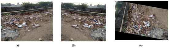
Figure 4. (a) Original Image (b) Horizontal Flipping (c) 120-degree Rotation.

The brightness augmentation technique is used to change the contrast of the sample image. Figure 5 represents the brightness augmentation of the sample image. Figure 5a,b represents the different levels of the brightness augmentation (0.2 and 2.0 respectively). The zoom augmentation is used to zoom the sample image at different levels. Figure 5c,d represents the zoom augmentation technique of the sample image at 0.4 and 0.8 levels of the zoom augmentation respectively.

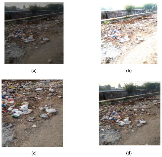
Figure 5. (a) 0.2 Brightness level (b) 2.0 Brightness level (c) 0.4 Zoom level (d) 0.8 Zoom level.

The size of the image data set is increased after applying the augmentation technique as the small image data set causes poor approximation. The deep learning models with small image data sets always suffer from the overfitting problem. Augmentation helps to generate new images and resolve the overfitting problem. In this study, approximately 5000 new images were generated after applying the augmentation technique. Table 2 shows the number of augmented dataset images.

Table 2. Sample Images Before and After Data Augmentation.

S.No.	Categories	Number of Images before Augmentation	Number of Images after Augmentation
1	Solid Waste Images	1000	3000
2	Clean Images	1000	3000

4. Proposed Methodology

Two CNN models for solid waste detection using an image dataset captured by the UAV were used. Table 3 shows the architecture description of the proposed models.

Table 3. CNN Model Architectures.

Models	Convolution Layers	Maxpool Layer	Parameters (in Millions)	Input Layer Size	Output Layer Size
CNN1	3	3	25	(224,224,3)	(2,1)
CNN2	5	5	16	(224,224,3)	(2,1)

The CNN1 model has three convolution layers and max pool layers as shown in the block diagram. One dropout layer is used to avoid overfitting. The flattening layer is used to flatten the input. The dense layer is the regularly deeply connected and frequently used layer. There are two dense layers used in CNN1. Table 4 shows the layer-wise description of the CNN1 model. The 224*224*3 sized images were used as the input to the proposed CNN1. In the convolution layer, the size of the filter was 3*3 and the number of the filter was 16. The output of the first convolution layer was 224*224*16. The max pool layer was used to reduce the size of the image. In the max pool layer, the 2*2 sized filter was used. The maxpool layer converted the input image size 224*224*16 into 112*112*16. The 112*112*16 sized image passed through the 2nd convolution layer from the max pool layer. The 2nd convolution layer had a 3*3 size filter and the number of the filter was 32. The output of the 2nd convolution layer was 112*112*32. The 2nd maxpool layer reduced the size of the image from 112*112*32 to 56*56*32. The output of the 2nd maxpool layer was then passed through the 3rd convolution layer. The 3rd convolution layer used 64 filters. Therefore, the output of the 3rd convolution layer was 56*56*64. The 3rd maxpool layer converted the output image size of the 3rd convolution layer into 28*28*64. The output of the 3rd maxpool layer was passed through the dropout and flatten layers. The dropout ratio of the dropout layer was 0.4. The dropout ratio of 0.4 describes that the 40% features out of total extracting features are neglected. The dense layer performed some operations on the input and returned the output.

Table 4. Layer Description of CNN1.

Sr. No.	Input Image Size	Layer Name	Filter Size	No. of Filter	No. of Parameter	Output Image Size
1.	224*224*3	Conv2D	3*3	16	448	224*224*16
2.	224*224*16	Maxpool Layer	2*2	-	-	112*112*16
3.	112*112*16	Conv2D	3*3	32	4640	112*112*32
4.	112*112*32	Maxpool Layer	2*2	-	-	56*56*32
5.	56*56*32	Conv2D	3*3	64	18,496	56*56*6
6.	56*56*64	Maxpool Layer	2*2	-	-	28*28*64
7.	28*28*64	Dropout Layer (0.4)	-	-	-	28*28*64
8.	28*28*64	Flatten Layer	-	-	-	50,176
9.	50,176	Dense Layer_1 (512)	-	-	25,690,624	512
10.	512	Dense Layer_2(1)	-	-	513	1

The block diagram of the proposed CNN2 model has five convolution layers and max pool layers. One dropout layer was used to avoid the overfitting problem. The flattening layer was used to flatten the input. The dense layer is the regularly deeply connected and frequently used layer. There were two dense layers used in CNN2.

Table 5 shows the layer-wise description of the CNN2 model. The image of 224*224*3 size was used as the input to the convolution layer with a filter size of 3*3.

Table 5. Layer Description of CNN2.

Sr. No.	Input Image Size	Layer Name	Filter Size	No. of Filter	No. of Parameter	Output Image Size
1.	224*224*3	Conv2D	3*3	16	448	224*224*16
2.	224*224*16	Maxpool Layer	2*2	-	-	112*112*16
3.	112*112*16	Conv2D	3*3	16	2320	112*112*16
4.	112*112*16	Maxpool Layer	2*2	-	-	56*56*16
5.	56*56*16	Conv2D	3*3	32	4640	56*56*32
6.	56*56*32	Maxpool Layer	2*2	-	-	28*28*32
7.	28*28*32	Conv2D	3*3	32	9248	28*28*32
8.	28*28*32	Maxpool Layer	2*2	-	-	14*14*32
9.	14*14*32	Conv2D	3*3	64	18,496	14*14*64
10.	14*14*64	Maxpool Layer	2*2	-	-	7*7*64
11.	7*7*64	Dropout Layer (0.4)	-	-	-	7*7*64
12.	7*7*64	Flatten Layer	-	-	-	3136
13.	3136	Dense Layer_1 (512)	-	-	1,606,144	512
14.	512	Dense Layer_2(1)	-	-	513	1

The number of the filter was 16. The output of the first convolution layer was 224*224*16 and was directly connected to the maxpool layer with a filter size of 2*2. The maxpool layer reduced the input image size from 224*224*16 to 112*112*16, which passed through the 2nd convolution layer with a filter size of 3*3. The number of the filter was 16. The output of the 2nd convolution layer was 112*112*16. The 2nd maxpool layer reduced the image from 112*112*16 to 56*56*16. The output of the 2nd maxpool layer passed through the 3rd convolution layer having 32 filters. The output of the 3rd convolution layer was 56*56*32, which was converted into 28*28*32 by the 3rd maxpool layer. The CNN2 model had two more convolution layers and maxpool layers. Therefore, after applying the convolution and maxpool operation, the size of the 5th maxpool layer was 14*14*7, which was passed through the dropout layer and flattening layer. The dropout ratio of the dropout layer was 0.4. The dense layer does the below operation on the input and returns the output.

5. Results and Analysis

The two models CNN1 and CNN2, designed for the experiment in this study, were trained on the solid waste image dataset. The proposed CNN models have only two classes, class-0 and class-1, resulting in a 2*2 confusion matrix for the training model. The confusion matrix contains some parameters like True Positive (TP), False Positive (FP), True Negative (TN) and False Negative (FN). The CNN1 and CNN2 performances were evaluated for different learning rates, optimizers and the number of epochs.

5.1. Results for Proposed Model CNN 1

The proposed model CNN1 performance was analyzed for different learning rates and the number of epochs at two different optimizers: RMSprop and Adam. Four learning rates (0.1, 0.001, 0.0001 and 0.00001) were considered for simulation to achieve the desired results. Moreover, three different epochs (10, 30 and 50) were taken for simulating the CNN1 model. All the simulations used a fixed batch size of 32.

5.1.1. Analysis with RMSPROP Optimizer

Table 6 shows the performance of the proposed model CNN1 using the RMSprop optimizer. The CNN1 model was trained on different learning rates and epochs. These learning rates and epochs were 0.1, 0.001, 0.0001, 0.00001 and 10, 30, 50 respectively. The best accuracy achieved by the RMSprop optimizer was 90% at a learning rate of 0.0001 with ten epochs. The highest precision value with the RMSprop optimizer was 0.86 in class-0 and 0.92 in class-1. The highest recall value achieved by the model CNN1 using RMSprop optimizer was 0.88 in class-0 and 0.91 in class-1. The RMSprop optimizer had the highest F1-score value of 0.87 in class-0 and 0.91 in class-1.

Table 6. Confusion Matrix Parameters of CNN1 Model with 32 Batch Size, RMSPROP Optimizer.

Epoch	Learning Rate	Precision		Recall		F-Score		Accuracy (Percentage)
		Class-0	Class-1	Class-0	Class-1	Class-0	Class-1
10	0.1	0.81	0.90	0.85	0.87	0.83	0.88	86
	0.001	0.00	0.61	0.00	0.67	0.00	0.76	60
	0.0001	0.86	0.92	0.88	0.91	0.87	0.91	90
	0.00001	0.76	0.68	0.26	0.70	0.42	0.81	73
30	0.1	0.00	0.61	0.00	0.70	0.00	0.76	61
	0.001	0.84	0.86	0.76	0.91	0.80	0.88	85
	0.0001	0.82	0.87	0.79	0.89	0.81	0.88	85
	0.00001	0.00	0.61	0.00	0.61	0.00	0.76	61
50	0.1	0.25	0.61	0.19	0.90	0.30	0.76	59
	0.001	0.86	0.84	0.74	0.92	0.79	0.88	85
	0.0001	0.81	0.90	0.85	0.87	0.83	0.88	86
	0.00001	0.80	0.68	0.26	0.75	0.42	0.81	75

5.1.2. Analysis with ADAM Optimizer

The performance of the proposed CNN1 using Adam optimizer is shown in Table 7. The best accuracy achieved by the CNN1 using Adam optimizer was 94% at a learning rate of 0.0001 with 30 epochs. The Adam optimizer had the highest precision value of 0.91 in class-0 and 0.96 in class-1. The highest recall value achieved by the model CNN1 using Adam optimizer was 0.94 in class-0 and 0.94 in class-1. The Adam optimizer yielded the highest F1-score value of 0.93 in class-0 and 0.95 in class-1.

Table 7. Confusion Matrix Parameters of CNN1 Model with 32 Batch Size, ADAM Optimizer.

Epoch	Learning Rate	Precision		Recall		F-Score		Accuracy (Percentage)
		Class-0	Class-1	Class-0	Class-1	Class-0	Class-1
10	0.1	0.84	0.94	0.91	0.89	0.87	0.91	90
	0.001	0.85	0.98	0.97	0.89	0.90	0.93	92
	0.0001	0.89	0.94	0.91	0.92	0.90	0.93	92
	0.00001	0.85	0.98	0.97	0.89	0.90	0.93	92
30	0.1	0.82	0.94	0.91	0.87	0.86	0.90	89
	0.001	0.89	0.94	0.91	0.92	0.90	0.93	92
	0.0001	0.91	0.96	0.94	0.94	0.93	0.95	94
	0.00001	0.94	0.93	0.88	0.96	0.91	0.94	93
50	0.1	0.76	0.96	0.94	0.81	0.84	0.88	86
	0.001	0.82	0.94	0.91	0.87	0.86	0.90	89
	0.0001	0.87	0.86	0.76	0.92	0.81	0.89	86
	0.00001	0.86	0.96	0.94	0.91	0.90	0.93	92

5.1.3. Comparison of RMSPROP and ADAM Optimizer

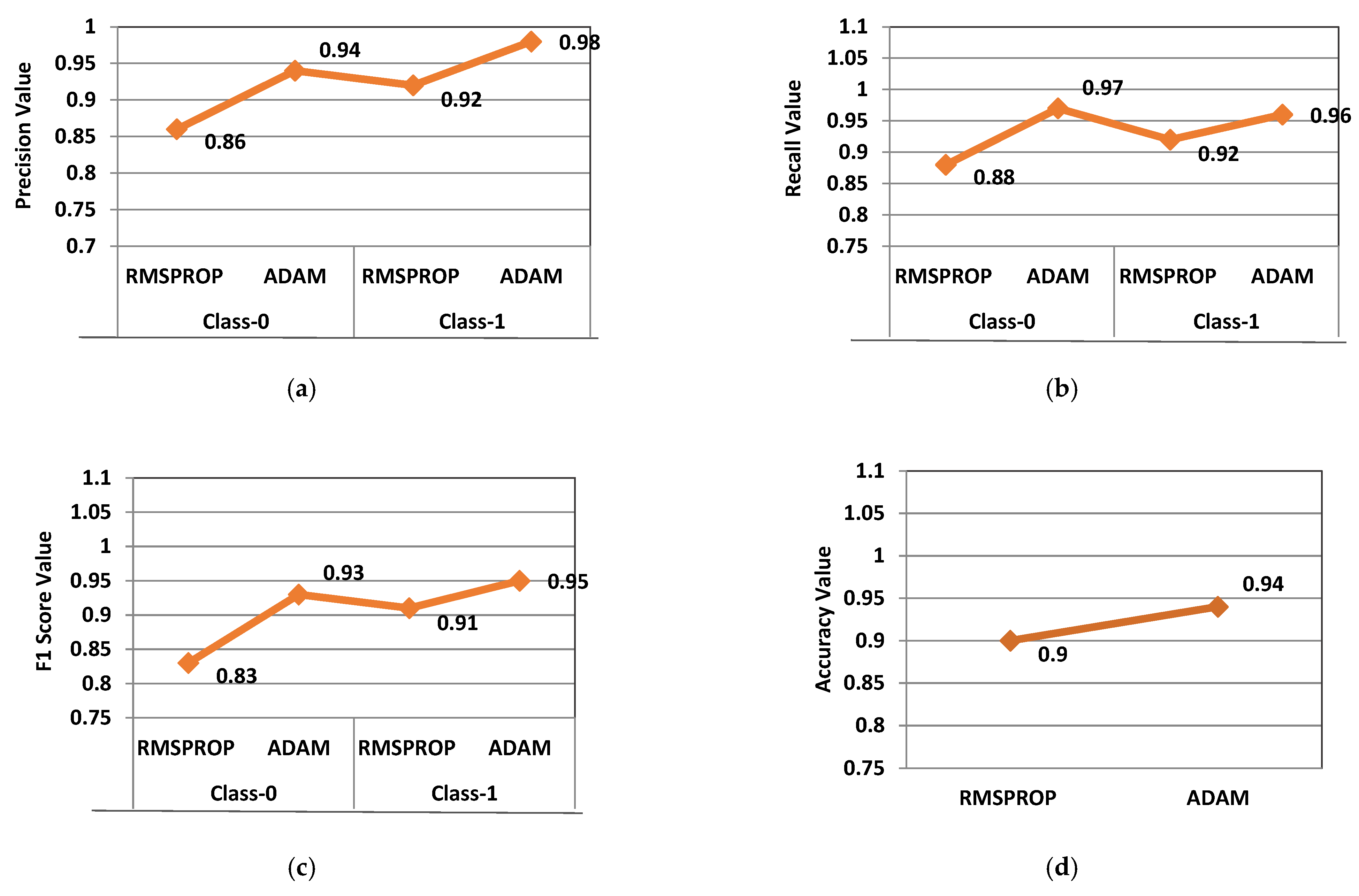
Figure 6 shows the comparison of the performance parameters of the CNN1 model with RMSprop and Adam optimizer. The precision value achieved by the CNN1 was best with Adam in class-1, whereas recall was highest in class-0 by Adam. The Adam optimizer yielded the highest F1-score value of 0.95 in class-1 and accuracy of 94%. RMSProp utilizes the 2nd moment with a decay rate to gain speed whereas Adam utilizes both the 1st and 2nd moment, which is why Adam is the better choice.

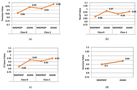
Figure 6. Confusion Matrix Parameter of CNN1 (a) Precision, (b) Recall, (c) F1-Score (d) Accuracy.

5.2. Results for Proposed Model CNN 2

The proposed model CNN2 performance was evaluated for different learning rates and the number of epochs at two different optimizers: RMSprop and Adam. Four learning rates (0.1, 0.001, 0.0001, and 0.00001) were considered for simulation to achieve the desired results. Moreover, three different epochs (10, 30, and 50) were taken for simulating the CNN2 model. All the simulations used a fixed batch size of 32.

5.2.1. Analysis with RMSPROP Optimizer

Table 8 shows the performance of the proposed model CNN2 using the RMSprop optimizer from which it can be easily analyzed that the best accuracy achieved by the RMSprop optimizer is 87% at a learning rate of 0.0001 with 30 epochs. The RMSprop optimizer had the highest precision value of 0.86 in class-0 and 0.92 in class-1. The highest recall value achieved by the model CNN2 using RMSprop optimizer was 0.88 in class-0 and 0.91 in class-1.

Table 8. Confusion Matrix Parameters of CNN2 Model with 32 Batch Size, RMSPROP Optimizer.

Epoch	Learning Rate	Precision		Recall		F-Score		Accuracy (Percentage)
		Class-0	Class-1	Class-0	Class-1	Class-0	Class-1
10	0.1	0.1	0.00	0.61	0.00	0.76	0.00	61
	0.001	0.81	0.90	0.85	0.87	0.83	0.88	85
	0.0001	0.82	0.87	0.79	0.89	0.81	0.88	85
	0.00001	0.69	0.68	0.26	0.61	0.42	0.81	75
30	0.1	0.81	0.90	0.85	0.87	0.83	0.88	86
	0.001	0.86	0.84	0.74	0.92	0.79	0.88	85
	0.0001	0.86	0.92	0.88	0.91	0.80	0.91	87
	0.00001	0.74	0.68	0.26	0.64	0.42	0.81	77
50	0.1	0.25	0.61	0.19	0.90	0.30	0.76	59
	0.001	0.84	0.86	0.76	0.91	0.80	0.88	85
	0.0001	0.87	0.92	0.88	0.91	0.87	0.89	85
	0.00001	0.81	0.85	0.76	0.89	0.79	0.89	81

5.2.2. Analysis with ADAM Optimizer

Table 9 shows the performance of the proposed CNN2 using Adam optimizer. The best accuracy achieved by CNN2 using Adam optimizer was 90% at a learning rate of 0.0001 with 30 epochs. The Adam optimizer had the highest precision value of 0.87 in class-0 and 0.93 in class-1. The highest recall value achieved by the model CNN2 using RMSprop optimizer was 0.88 in class-0 and 0.93 in class-1. The Adam optimizer had the highest F1-score value of 0.89 in class-0 and 0.91 in class-1.

Table 9. Confusion Matrix Parameters of CNN2 Model with 32 Batch Size with ADAM Optimizer.

Epoch	Learning Rate	Precision		Recall		F-Score		Accuracy (Percentage)
		Class-0	Class-1	Class-0	Class-1	Class-0	Class-1
10	0.1	0.39	0.00	0.00	0.00	0.56	0.00	39
	0.001	0.84	0.87	0.79	0.91	0.82	0.89	86
	0.0001	0.79	0.94	0.91	0.85	0.85	0.89	87
	0.00001	0.78	0.84	0.74	0.87	0.76	0.85	82
30	0.1	0.39	0.00	0.61	0.00	0.56	0.00	39
	0.001	0.88	0.82	0.68	0.94	0.77	0.88	84
	0.0001	0.87	0.93	0.88	0.93	0.89	0.91	90
	0.00001	0.86	0.84	0.74	0.92	0.79	0.88	85
50	0.1	0.00	0.61	0.00	0.70	0.00	0.76	61
	0.001	0.86	0.83	0.71	0.92	0.77	0.88	84
	0.0001	0.86	0.84	0.74	0.92	0.79	0.88	85
	0.00001	0.81	0.90	0.85	0.87	0.83	0.91	86

5.2.3. Comparison of RMSprop and Adam Optimizer

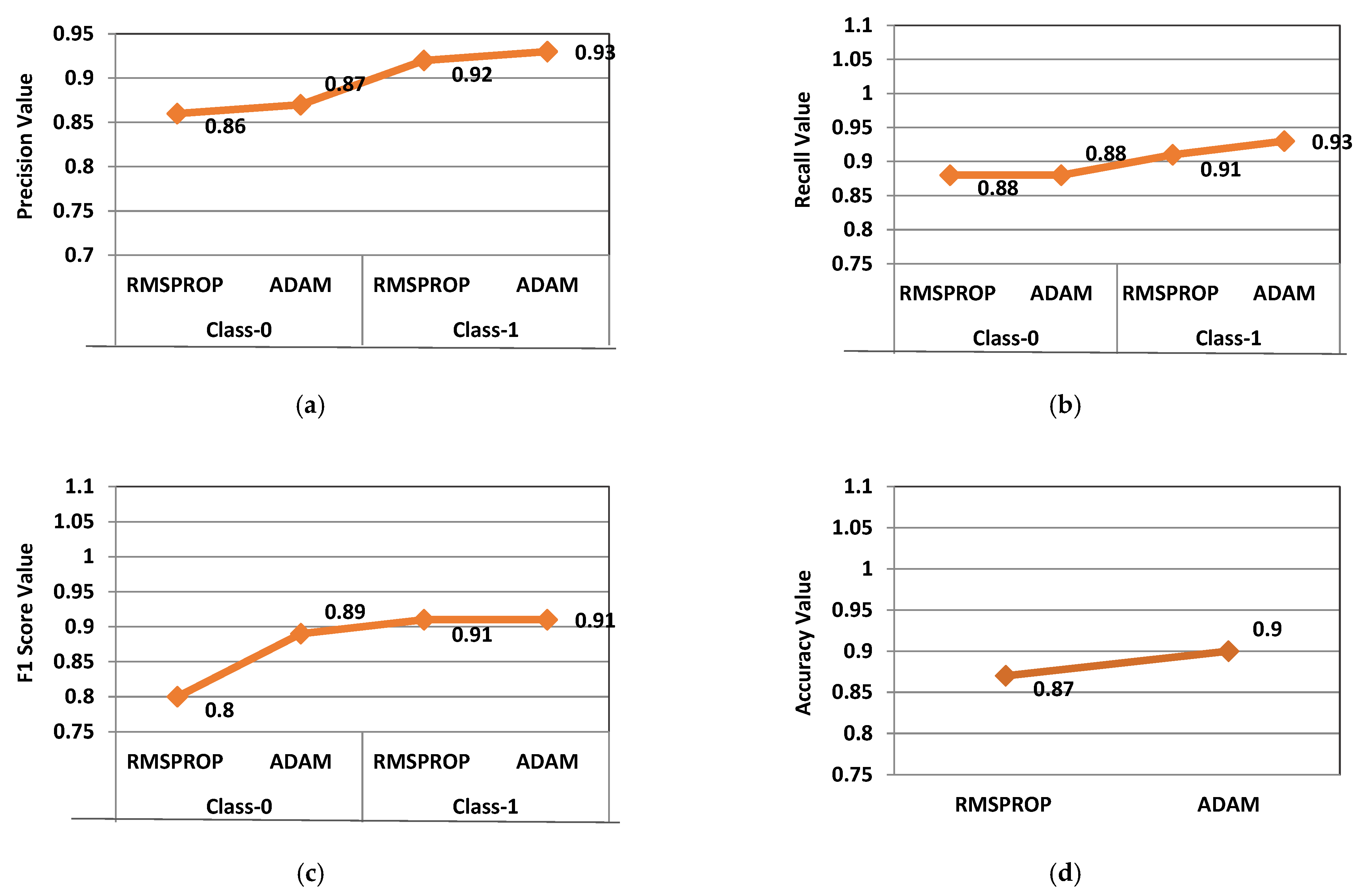
Figure 7 shows the comparison of the performance parameters of the CNN2 model with RMSprop and Adam optimizer. The precision value achieved by the CNN2 was best with Adam in class-1, whereas recall was highest in class-1 by Adam. The Adam optimizer gives the accuracy 90%, whereas RMSprop gives 87%. When the learning rate is small enough, RMSProp averages the gradients over subsequent mini-batches, which is why RMSProp is not a good choice.

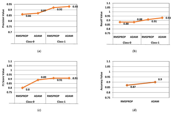
Figure 7. Confusion Matrix Parameter of CNN2 (a) Precision, (b) Recall, (c) F1-Score (d) Accuracy.

Figure 7a represents the precision plot of the model CNN2 using RMSprop and Adam optimizer. The Adam optimizer over-performed the RMSprop optimizer in terms of precision. The precision value of the RMSprop optimizer was 0.86 in class-0 and 0.92 in class-1 and for the Adam optimizer, it was 0.87 in class-0 and 0.93 in class-1. Figure 7b represents the recall plot of the CNN2 model for both optimizers. The Adam optimizer also delivered a better performance than the RMSprop optimizer in terms of precision. The recall value achieved using the RMSprop optimizer was 0.88 in class-0 and 0.91 in class-1, while with Adam optimizer, it was 0.88 in class-0 and 0.93 in class-1. Figure 7c represents the F1-score plot of model CNN2. The highest F1-score value achieved using the RMSprop optimizer by the CNN2 model was 0.80 in class-0 and 0.91 in class-1, while with Adam optimizer, it was 0.89 in class-0 and 0.91 in class-1. Figure 7d represents the overall accuracy achieved by the CNN2 model. The Adam optimizer has achieved 87% accuracy, while the RMSprop optimizer achieved 90% accuracy. Adam optimizer achieved a higher performance efficiency than the RMSprop optimizer.

5.3. Comparison of the Proposed Models

Both the models yielded their best performance on the Adam optimizer as it itself learns all the learning rates. When the problem is large with multiple parameters, Adam optimizer is efficient. Figure 8 depicts the comparison of performances of CNN1 and CNN2 with Adam optimizer. The CNN1 model delivered better performance than the CNN2 model. The CNN1 model yielded the highest value of precision, recall, and F1-score at 0.96, 0.94, and 0.95 respectively. CNN1 also outperformed CNN2 in terms of accuracy: 94% at a learning rate of 0.0001 with an epoch size of 30. When epochs decreased, the F-score and accuracy increased and when epochs increased, the validation error increased, which led to overfitting, which is why 30 epochs are considered best in this scenario. In addition, the decreasing learning rate increases the risk of overfitting, so a learning rate of 0.0001 is considered best for the CNN1 model. CNN2 achieved 90% accuracy with the same simulation parameters.

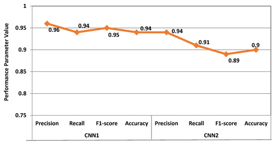
Figure 8. Comparison Analysis of Performance of CNN1 and CNN2.

5.4. Comparison of Proposed Model CNN1 with the State of Art

The below table shows the comparison of the proposed work with state-of-the-art approaches. Table 10 represents the accuracy results obtained for the various scripts.

Table 10. Comparison with Existing State-of-Art Models.

Reference	Convolution Neural Network	No. of Images	No. of Classes	Accuracy %
[2]	Scratch CNN Model	1312	2	83.33
[6]	VGG-16	2527	4	86.6
[9]	Artificial Neural Network	3046	3	67
[10]	Dense Net	600	5	83.7
[11]	Multilayer Hybrid System (MHS), Alex Net	5000	6	90
[12]	VGG-16, Alex Net	2400	4	93
Proposed Model CNN1	CNN1 Model	6000	2	94%

6. Conclusions and Future Scope

Two CNN models named CNN1 and CNN2 were evaluated for solid waste detection. These models were trained on a solid waste image data set based on deep learning and application of symmetry. The author analyzed the performance of CNN models using Adam and RMSprop optimizer at a learning rate of 0.0001, 30 epochs and 32 batch sizes. The Adam optimizer performed better than the RMSprop optimizer. The proposed model CNN1 achieved higher accuracy of 94% than model CNN2 with Adam optimizer. This comparative study would benefit the municipal corporation by saving money and time in garbage collection. Deep CNN is a trendy research topic. The application of deep CNN in unsupervised learning is likely in the future too. The deep CNN technologies have made excellent progress in computer vision. Most of the deep CNN progress is not for the full power hardware or bigger data sets but mainly for the rapid inventions of new algorithms and improved architecture of the networks. This proposed CNN model could become an alternate choice for the municipal corporations and help monitoring the landfill sites. This study demonstrates the potential of the neural network and symmetry in improving the efficiency of waste management so that it is economical and environmentally beneficial for our society.

References

- Singh, A. Managing the uncertainty problems of municipal solid waste disposal. J. Environ. Manag. 2019, 240, 259–265. [Google Scholar] [CrossRef] [PubMed]
- Jakovljevic, G.; Govedarica, M.; Alvarez-Taboada, F. A deep learning model for automatic plastic mapping using unmanned aerial vehicle (UAV) data. Remote Sens. 2020, 12, 1515. [Google Scholar] [CrossRef]
- Hong, S.J.; Han, Y.; Kim, S.Y.; Lee, A.Y.; Kim, G. Application of Deep-Learning Methods to Bird Detection Using Unmanned Aerial Vehicle Imagery. Sensors 2019, 19, 1651. [Google Scholar] [CrossRef] [PubMed] [Green Version]
- Ronneberger, O.; Fischer, P.; Brox, T. U-net: Convolutional networks for biomedical image segmentation. In Proceedings of the International Conference on Medical Image Computing and Computer-Assisted Intervention, Munich, Germany, 5–9 October 2015; Springer: Cham, Switzerland, 2015; pp. 234–241. [Google Scholar]
- Chang, M.; Xing, Y.Y.; ZhanG, Q.Y.; Han, S.J.; Kim, M. A CNN Image Classification Analysis for ‘Clean-Coast Detector’ as Tourism Service Distribution. J. Distrib. Sci. 2020, 18, 15–26. [Google Scholar] [CrossRef]
- Kujawa, S.; Mazurkiewicz, J.; Czekała, W. Using convolutional neural networks to classify the maturity of compost based on sewage sludge and rapeseed straw. J. Clean. Prod. 2020, 258, 120814. [Google Scholar] [CrossRef]
- Xu, X.; Qi, X.; Diao, X. Reach on waste classification and identification by transfer learning and lightweight neural network. Comput. Sci. 2020. [Google Scholar]
- Toğaçar, M.; Ergen, B.; Cömert, Z. Waste classification using AutoEncoder network with integrated feature selection method in con;volutional neural network models. Measurement 2020, 153, 107459. [Google Scholar] [CrossRef]
- Vo, A.H.; Vo, M.T.; Le, T. A novel framework for trash classification using deep transfer learning. IEEE Access 2019, 7, 178631–178639. [Google Scholar] [CrossRef]
- Ruiz, V.; Sánchez, Á.; Vélez, J.F.; Raducanu, B. Automatic image-based waste classification. In Proceedings of the International Work-Conference on the Interplay Between Natural and Artificial Computation, Almeria, Spain, 3–7 June 2019; Springer: Cham, Switzerland, 2019; pp. 422–431. [Google Scholar]
- Bobulski, J.; Kubanek, M. Waste classification system using image processing and convolutional neural networks. In Proceedings of the International Work-Conference on Artificial Neural Networks, Gran Canaria, Spain, 12–14 June 2019; Springer: Cham, Switzerland, 2019; pp. 350–361. [Google Scholar]
- Gyawali, D.; Regmi, A.; Shakya, A.; Gautam, A.; Shrestha, S. Comparative analysis of multiple deep CNN models for waste classification. arXiv 2020, arXiv:2004.02168. [Google Scholar]
- Gupta, P.K.; Shree, V.; Hiremath, L.; Rajendran, S. The Use of Modern Technology in Smart Waste Management and Recycling: Artificial Intelligence and Machine Learning. In Recent Advances in Computational Intelligence; Springer: Cham, Switzerland, 2019; pp. 173–188. [Google Scholar]
- Huiyu, L.; Owolabi Ganiyat, O.; Kim, S.H. Automatic Classifications and Recognition for Recycled Garbage by Utilizing Deep Learning Technology. In Proceedings of the 2019 7th International Conference on Information Technology: IoT and Smart City, Chennai, India, 11–15 March 2019; pp. 1–4. [Google Scholar]
- Chu, Y.; Hung, C.; Xie, X.; Tan, B.; Kamal, S.; Xiong, X. Multilayer hybrid deep-learning method for waste classification and recycling. Comput. Intell. Neurosci. 2018, 2018, 5060857. [Google Scholar] [CrossRef] [Green Version]
- Costa, B.S.; Bernardes, A.C.; Pereira, J.V.; Zampa, V.H.; Pereira, V.A.; Matos, G.F.; Soares, E.A.; Soares, C.L.; Silva, A.F. Artificial intelligence in automated sorting in trash recycling. In Proceedings of the Anais do XV Encontro Nacional de Inteligência Artificial e Computacional, Sao Paolo, Brasil, 22–25 October 2018; SBC: New Delhi, India, 2018; pp. 198–205. [Google Scholar]
- Zhao, X.; Yuan, Y.; Song, M.; Ding, Y.; Lin, F.; Liang, D.; Zhang, D. Use of Unmanned Aerial Vehicle Imagery and Deep Learning UNet to Extract Rice Lodging. Sensors 2019, 19, 3859. [Google Scholar] [CrossRef] [PubMed] [Green Version]
- Soundarya, B.; Parkavi, K.; Sharmila, A.; Kokiladevi, R.; Dharani, M.; Krishnaraj, R. CNN Based Smart Bin for Waste Management. In Proceedings of the 2022 4th International Conference on Smart Systems and Inventive Technology (ICSSIT), Tirunelveli, India, 20–22 January 2022; pp. 1405–1409. [Google Scholar]
- Yi, Y.; Zhang, Z.; Zhang, W.; Zhang, C.; Li, W.; Zhao, T. Semantic Segmentation of Urban Buildings from VHR Remote Sensing Imagery Using a Deep Convolutional Neural Network. Remote Sens. 2019, 11, 1774. [Google Scholar] [CrossRef] [Green Version]
- Ahmad, K.; Khan, K.; AI-Fuqaha, A. Intelligent Fusion of Deep Features for Improved Waste Classification. IEEE Access 2020, 8, 96495–96504. [Google Scholar] [CrossRef]
- Altikat, A.A.A.G.S.; Gulbe, A.; Altikat, S. Intelligent solid waste classification using deep convolutional neural networks. Int. J. Environ. Sci. Technol. 2021, 19, 1–8. [Google Scholar] [CrossRef]
- Seredkin, A.V.; Tokarev, M.P.; Plohih, I.A.; Gobyzov, O.A.; Markovich, D.M. Development of a method of detection and classification of waste objects on a conveyor for a robotic sorting system. J. Phys. Conf. Ser. 2019, 1359, 012127. [Google Scholar] [CrossRef] [Green Version]
- Wang, Y.; Zhao, W.J.; Xu, J.; Hong, R. Recyclable Waste Identification Using CNN Image Recognition and Gaussian Clustering. arXiv 2020, arXiv:2011.01353. [Google Scholar]
- Zhang, Z.; Wang, H.; Song, H.; Zhang, S.; Zhang, J. Industrial Robot Sorting System for Municipal Solid Waste. In Proceedings of the International Conference on Intelligent Robotics and Applications, Macau, India, 4–8 November 2019; Springer: Cham, Switzerland, 2019; pp. 342–353. [Google Scholar]
- Brintha, V.P.; Rekha, R.; Nandhini, J.; Sreekaarthick, N.; Ishwaryaa, B.; Rahul, R. Automatic Classification of Solid Waste Using Deep Learning. In Proceedings of the International Conference on Artificial Intelligence, Smart Grid and Smart City Applications, Macau, India, 5 October 2019; Springer: Cham, Switzerland, 2019; pp. 881–889. [Google Scholar]
- Mudita; Gupta, D. Prediction of Sensor Faults and Outliers in IoT Devices. In Proceedings of the 2021 9th International Conference on Reliability, Infocom Technologies and Optimization (Trends and Future Directions), Noida, India, 3–4 September 2021; pp. 1–5. [Google Scholar]
- Moreira, R.; Teles, A.; Fialho, R.; Baluz, R.; Santos, T.C.; Goulart-Filho, R.; Rocha, L.; Silva, F.J.; Gupta, N.; Bastos, V.H.; et al. Mobile Applications for Assessing Human Posture: A Systematic Literature Review. Electronics 2020, 9, 1196. [Google Scholar] [CrossRef]
- Uppal, M.; Gupta, D.; Juneja, S.; Dhiman, G.; Kautish, S. Cloud-Based Fault Prediction Using IoT in Office Automation for Improvisation of Health of Employees. J. Healthc. Eng. 2021, 2021, 8106467. [Google Scholar] [CrossRef]
- Singh, T.P.; Gupta, S.; Garg, M.; Gupta, D.; Alharbi, A.; Alyami, H.; Anand, D.; Ortega-Mansilla, A.; Goyal, N. Visualization of Customized Convolutional Neural Network for Natural Language Recognition. Sensors 2022, 22, 2881. [Google Scholar] [CrossRef]
- Uppal, M.; Gupta, D.; Anand, D.; Alharithi, F.S.; Almotiri, J.; Mansilla, A.; Singh, D.; Goyal, N. Fault pattern diagnosis and classification in sensor nodes using fall curve. Comput. Mater. Contin. 2022, 72, 1799–1814. [Google Scholar] [CrossRef]
- Malik, S.; Gupta, K.; Gupta, D.; Singh, A.; Ibrahim, M.; Ortega-Mansilla, A.; Goyal, N.; Hamam, H. Intelligent Load-Balancing Framework for Fog-Enabled Communication in Healthcare. Electronics 2022, 11, 566. [Google Scholar] [CrossRef]
- Garcia-Garin, O.; Monleón-Getino, T.; López-Brosa, P.; Borrell, A.; Aguilar, A.; Borja-Robalino, R.; Cardona, L.; Vighi, M. Automatic detection and quantification of floating marine macro-litter in aerial images: Introducing a novel deep learning approach connected to a web application in R. Environ. Pollut. 2021, 273, 116490. [Google Scholar] [CrossRef] [PubMed]
- Sliusar, N.; Filkin, T.; Huber-Humer, M.; Ritzkowski, M. Drone technology in municipal solid waste management and landfilling: A comprehensive review. Waste Manag. 2022, 139, 1–16. [Google Scholar] [CrossRef] [PubMed]
Publisher’s Note: MDPI stays neutral with regard to jurisdictional claims in published maps and institutional affiliations. |
© 2022 by the authors. Licensee MDPI, Basel, Switzerland. This article is an open access article distributed under the terms and conditions of the Creative Commons Attribution (CC BY) license (https://creativecommons.org/licenses/by/4.0/).