An Efficient Red–Black Skewed Modified Accelerated Arithmetic Mean Iterative Method for Solving Two-Dimensional Poisson Equation

Abstract

This paper presents the extended variants to the established two-stage Arithmetic Mean (AM) method known as the Modified Accelerated Arithmetic Mean (MAAM) and Skewed Modified Accelerated Arithmetic Mean (SkMAAM) methods to solve the two-dimensional elliptic problem. The existing two-stage AM and its skewed variants apply one weighted parameter for the computation of nodes in Levels 1 and 2. The suggested MAAM and SkMAAM methods employ red–black ordering with two different weighted parameters and an additional two distinct accelerated parameters for red and black nodes, respectively. By carefully choosing optimum parameter values, the proposed MAAM and SkMAAM improve the computational execution of the algorithm. With red–black ordering, the computational molecules of red and black nodes are symmetrical, in which the computation of red nodes applies the updated values of their four neighbouring black nodes and vice versa. These symmetrical computational molecules of red and black nodes can be seen for the modified variants MAM and MAAM, and their corresponding skewed variants SkMAM and SkMAAM. The proposed MAAM and SkMAAM methods are compared to the existing AM and Modified AM (MAM) and their corresponding skewed variants, namely the Skewed AM (SkAM) and Skewed MAM (SkMAM) methods. The performance of the newly proposed MAAM and SkMAAM methods is compared against the existing methods in terms of computational complexity and actual execution time. It is shown in the simulation results that the skewed variants are superior to their corresponding regular variants, in which the SkMAAM method gives the best performance.

1. Introduction

The two-stage iterative methods had been studied extensively in the past to solve linear system problems [1]. In [2], a two-stage method known as the Arithmetic Mean (AM) method was introduced. The AM method was applied recently to solve a linear Fredholm integral equation [3]. In [4], a variant of a two-stage approach based on the Alternating Decomposition Explicit method was explored to solve the diffusion equation. An application of the two-stage arithmetic method to solve the glioma growth model was presented in [5]. A combination of AM and Newton methods was reported in [3]. In [6], Sulaiman et al. introduced the Half-Sweep Arithmetic Mean method, in which the half-sweep approach has been successfully applied on the skewed grid to reduce the computational complexity drastically. The existing variants of the AM method employ a weighted parameter to speed up the convergence rate. This sole weighted parameter method, also widely known as the Successive Overrelaxation (SOR) method, was extensively studied by Young [7] to solve the partial differential equation of elliptic type and its impact in the 20th century was presented in [8].

In recent studies, the SOR and its variants were applied to solve problems in image processing [9] and agent navigation [10]. An extension to the SOR known as the Accelerated Overrelaxation (AOR) method that employs two acceleration parameters was later introduced by Hadjidimos [11]. As pointed out in [11], if fully exploited, the presence of two parameters in AOR and its variant [12,13] will provide a faster convergence rate than any other methods of the same type. Moreover, the red–black ordering strategy was applied in a previous work where two different weighted parameters were used for the calculation of red and black nodes to improve the execution time [14,15]. It is interesting to note that the numerical solutions to the fractional version of the partial differential equation were actively studied in recent works. Ali and Abdullah [16] proposed an implicit finite difference method to solve a one-dimensional wave equation. In [17], an efficient computational approach for a local fractional Poisson equation in fractal media was suggested. In future work, we aim to consider employing the two-stage iterative methods for solving fractional partial differential equations.

In this study, we introduced two variants of AM methods, namely the MAAM and SkMAAM methods, for solving elliptic partial differential equations in two-dimensional space. We applied the AOR scheme to the existing AM method to construct a new variant of the AM method known as the Modified Accelerated Arithmetic Method (MAAM) method, which is implemented on a regular grid using a red–black ordering strategy. Apart from MAAM, its variant, namely the Skewed Modified Accelerated Arithmetic Method (SkMAAM), was implemented on the skewed grid. It is widely known that the half-sweep approach can be applied to the skewed grid, which is capable of reducing the amount of computation by half.

In our previous work, the half-sweep variants of the AM and MAM methods, known as Half-Sweep AM (HSAM) [18] and Half-Sweep MAM (HSMAM) [19], were applied to solve the two-dimensional elliptic equation. The performance of the proposed MAAM and SkMAAM methods was compared with the AM and MAM methods, and the current state-of-the-art HSAM method (also known as the SkAM method) and SkMAM method. The encouraging results given by the two-stage iterative methods motivate us to develop an extension to the previous work. All skewed variants considered in this study apply the rotated grid to reduce the amount of computation. Thus, the main contribution of this work is that the newly proposed MAAM and SkMAAM methods introduce the use of accelerated parameters that are shown to provide faster convergence when optimum values are chosen.

The description of the finite difference methods of SOR and AOR is provided in Section 2. In Section 3, we present the description of the existing AM method and its skewed variant in two-dimensional space implementation. The MAM and SkMAM methods are also presented in Section 3. In Section 4, we describe the proposed MAAM and SkMAAM methods and explain the implementation of both methods for computing the solution of the elliptic equation. The novelty of the proposed methods by introducing additional different accelerated parameters for red and black nodes is explained. The obtained numerical results are provided and summarised in Section 5. The computational complexities of the considered iterative methods are discussed in Section 5. Finally, the conclusions are drawn in Section 6.

2. Finite Difference Approximation Equations

By considering the following elliptic boundary value problem

$${\nabla }^{2}u=\frac{{\partial }^{2}u}{\partial x^2}+\frac{{\partial }^{2}u}{\partial y^2}=f(x,y),(x,y)\in \mathrm{\Omega },$$

(1)

with Dirichlet boundary conditions

$$u(x,y)=g(x,y),(x,y)\in \partial \mathrm{\Omega },$$

(2)

where $\mathrm{\Omega }$ is a bounded region in ${\Re }^2$. The finite difference method is used to discretise the Poisson Equation (1), which is often applied to model the phenomena of fluid dynamics and heat conduction processes. Equation (1) can be approximated using the standard five-point difference approximation formula given as

$$u_{i-1,j}+u_{i+1,j}+u_{i,j-1}+u_{i,j+1}-4u_{i,j}=h^2{f}_{i,j},$$

(3)

where h denotes the spacing between node points in i and j directions of a rectangular grid.

If the axis of the rectangular grid is rotated by ${45}^{\circ }$ [20], we can obtain the skewed five-point difference approximation formula given as

$$u_{i-1,j-1}+u_{i+1,j-1}+u_{i-1,j+1}+u_{i+1,j+1}-4u_{i,j}=2h^2{f}_{i,j}.$$

(4)

Equations (3) and (4) are then used for the iterative methods implemented on the regular or skewed grids. Accordingly, the iterative schemes for the standard five-point difference formula on the regular and skewed grids can be written as

$$\begin{array}{cc}\hfill u_{i,j}^{(k+1)}& =\frac{1}{4}\left(u_{i-1,j}^{(k+1)}+u_{i+1,j}^{\left(k\right)}+u_{i,j-1}^{(k+1)}+u_{i,j+1}^{\left(k\right)}-h^2{f}_{i,j}\right)\hfill \end{array}$$

(5)

and

$$\begin{array}{cc}\hfill u_{i,j}^{(k+1)}& =\frac{1}{4}\left(u_{i-1,j-1}^{(k+1)}+u_{i+1,j-1}^{(k+1)}+u_{i-1,j+1}^{\left(k\right)}+u_{i+1,j+1}^{\left(k\right)}-2h^2{f}_{i,j}\right),\hfill \end{array}$$

(6)

respectively. Consequently, the SOR iterative schemes for the corresponding regular and skewed five-point difference formula can be expressed as

$$\begin{array}{cc}\hfill u_{i,j}^{(k+1)}& =\frac{\omega }{4}\left(u_{i-1,j}^{(k+1)}+u_{i+1,j}^{\left(k\right)}+u_{i,j-1}^{(k+1)}+u_{i,j+1}^{\left(k\right)}-h^2{f}_{i,j}\right)+(1-\omega )u_{i,j}^{\left(k\right)},\hfill \end{array}$$

(7)

$$\begin{array}{cc}\hfill u_{i,j}^{(k+1)}& =\frac{\omega }{4}\left(u_{i-1,j-1}^{(k+1)}+u_{i+1,j-1}^{(k+1)}+u_{i-1,j+1}^{\left(k\right)}+u_{i+1,j+1}^{\left(k\right)}-2h^2{f}_{i,j}\right)+(1-\omega )u_{i,j}^{\left(k\right)}.\hfill \end{array}$$

(8)

As defined by Hadjidimos [11], to obtain the AOR iterative scheme for the standard five-point approximation, we replace $u_{i-1,j}^{(k+1)}$ and $u_{i,j-1}^{(k+1)}$ with $u_{i-1,j}^{\left(k\right)}$ and $u_{i,j-1}^{\left(k\right)}$, respectively, and add the terms $\frac{r}{4}(u_{i-1,j}^{(k+1)}-u_{i-1,j}^{\left(k\right)})$ and $\frac{r}{4}(u_{i,j-1}^{(k+1)}-u_{i,j-1}^{\left(k\right)})$. Hence, the AOR iterative scheme for the standard five-point formula on the regular grid can be written as

$$\begin{array}{cc}\hfill u_{i,j}^{(k+1)}=& \frac{\omega }{4}\left(u_{i-1,j}^{\left(k\right)}+u_{i+1,j}^{\left(k\right)}+u_{i,j-1}^{\left(k\right)}+u_{i,j+1}^{\left(k\right)}-h^2{f}_{i,j}\right)+(1-\omega )u_{i,j}^{\left(k\right)}+\hfill \\ \hfill & \frac{r}{4}\left(u_{i-1,j}^{(k+1)}-u_{i-1,j}^{\left(k\right)}+u_{i,j-1}^{(k+1)}-u_{i,j-1}^{\left(k\right)}\right).\hfill \end{array}$$

(9)

Similarly, the AOR iterative scheme for the five-point difference formula on the skewed grid can be constructed and is given as

$$\begin{array}{cc}\hfill u_{i,j}^{(k+1)}=& \frac{\omega }{4}\left(u_{i-1,j-1}^{\left(k\right)}+u_{i+1,j-1}^{\left(k\right)}+u_{i-1,j+1}^{\left(k\right)}+u_{i+1,j+1}^{\left(k\right)}-2h^2{f}_{i,j}\right)+(1-\omega )u_{i,j}^{\left(k\right)}\hfill \\ \hfill & \frac{r}{4}\left(u_{i-1,j-1}^{(k+1)}-u_{i-1,j-1}^{\left(k\right)}+u_{i+1,j-1}^{(k+1)}-u_{i+1,j-1}^{\left(k\right)}\right).\hfill \end{array}$$

(10)

The application of these finite difference Formulae (5)–(10) to approximate problem (1) will generate a large and sparse linear system that can be stated in matrix form as

$$Au=f$$

(11)

where A and f are known, and u is unknown. Matrix A can be decomposed into

$$A=D-L-T$$

(12)

where D, L and T are diagonal, strictly lower and strictly upper triangular matrices, respectively. The general iterative scheme of the generated linear system can be written as

$$\begin{array}{ccc}\hfill D{u}^{(k+1)}& =L{u}^{(k+1)}+T{u}^{\left(k\right)}+D{u}^{\left(k\right)}+f\hfill & \hfill \\ \hfill & =L{u}^{(k+1)}+(T+D)u^{\left(k\right)}+f.\hfill \end{array}$$

(13)

Accordingly, the SOR iterative scheme can be written as

$$\begin{array}{ccc}\hfill D{u}^{(k+1)}& =\omega L{u}^{(k+1)}+\omega T{u}^{\left(k\right)}+(1-\omega )D{u}^{\left(k\right)}+\omega f\hfill & \hfill \\ \hfill & =\omega L{u}^{(k+1)}+(\omega T+(1-\omega )D)u^{\left(k\right)}+\omega f.\hfill \end{array}$$

(14)

The AOR formula may be obtained from (14) by replacing $\omega L{u}^{(k+1)}$ with $\omega L{u}^{\left(k\right)}$ and adding the term $rL(u^{(k+1)}-u^{\left(k\right)})$ as shown below:

$$\begin{array}{ccc}\hfill D{u}^{(k+1)}& =\omega L{u}^{\left(k\right)}+\omega T{u}^{\left(k\right)}+(1-\omega )D{u}^{\left(k\right)}+\omega f+rL(u^{(k+1)}-u^{\left(k\right)})\hfill & \hfill \\ \hfill & =(\omega L+\omega T+(1-\omega )D)u^{\left(k\right)}+\omega f+rL(u^{(k+1)}-u^{\left(k\right)}).\hfill \end{array}$$

(15)

From now on, we shall call $\omega$ the weighted parameter and r the acceleration parameter. Furthermore, it can be noted that the AOR can be treated as an extrapolation of the SOR method with overrelaxation parameter r and extrapolation parameter $s=\omega /r$, as described in [11]. From Equations (13)–(15), $u^{(k+1)}$ denotes the unknown vector at iteration $(k+1)$, which we attempt to compute efficiently.

The classical Equation (13) does not provide a convergence optimisation mechanism. In Equation (14), the SOR scheme provides one overrelaxation parameter only to speed up the rate of convergence. Using Equation (15), two parameters can be adjusted to obtain the optimal convergence rate for solving the problem (1). Different values of $\omega$ and r can be chosen within the range between 1 and 2, in which good parameter values will give an acceptable optimum number of iterations.

3. Arithmetic Mean (AM) Method

The iterative process of the two-stage AM iterative method involves solving two independent systems such as ${\widehat{u}}^{\left(1\right)}$ and ${\widehat{u}}^{\left(2\right)}$, which are calculated at Levels 1 and 2, respectively. The average sum of the two matrices is computed at Level 3. By applying Equation (14), the general iterative scheme for the AM method can be defined as

$$\left.\begin{array}{cc}\hfill D{\widehat{u}}^{\left(1\right)}& =\omega (L{\widehat{u}}^{\left(1\right)}+T{u}^{\left(k\right)})+(1-\omega )D{u}^{\left(k\right)}+\omega f,\hfill \\ \hfill D{\widehat{u}}^{\left(2\right)}& =\omega (L{u}^{\left(k\right)}+T{\widehat{u}}^{\left(2\right)})+(1-\omega )D{u}^{\left(k\right)}+\omega f,\hfill \\ \hfill u^{(k+1)}& =\frac{1}{2}\left({\widehat{u}}^{\left(1\right)}+{\widehat{u}}^{\left(2\right)}\right),\hfill \end{array}\right\}$$

(16)

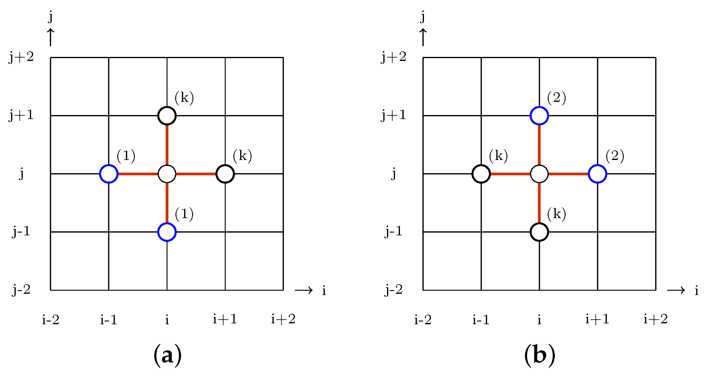
where the optimal value of the weighted parameter is in the range $1<\omega <2$. Note that if $\omega =1$, the standard Gauss–Seidel method is obtained. From Equation (16), it can be seen that the formulae applied in Levels 1 and 2 are symmetrical, as illustrated in the portion of the computational grid of the regular and skewed cases shown in Figure 1 and Figure 2, respectively.

The iterative method (16) is known to have well-defined structures that are suitable for parallel implementation [21]. The lower triangular system and the upper triangular system in this method can be executed independently on two different processors. The convergence proof of the iterative method is described in the following theorems [21].

Theorem 1.

Let $A=\left(a_{ij}\right)$ be an $N\times N$ irreducibly diagonally dominant matrix with $a_{ij}\le 0$, for all $i\ne j$ and $a_{ii}>0,i=1,2,\dots ,n$. Then, the iterative method (16) is convergent for all $0<\omega <2$.

Proof of Theorem 1. 

A detailed proof is described in [21].    □

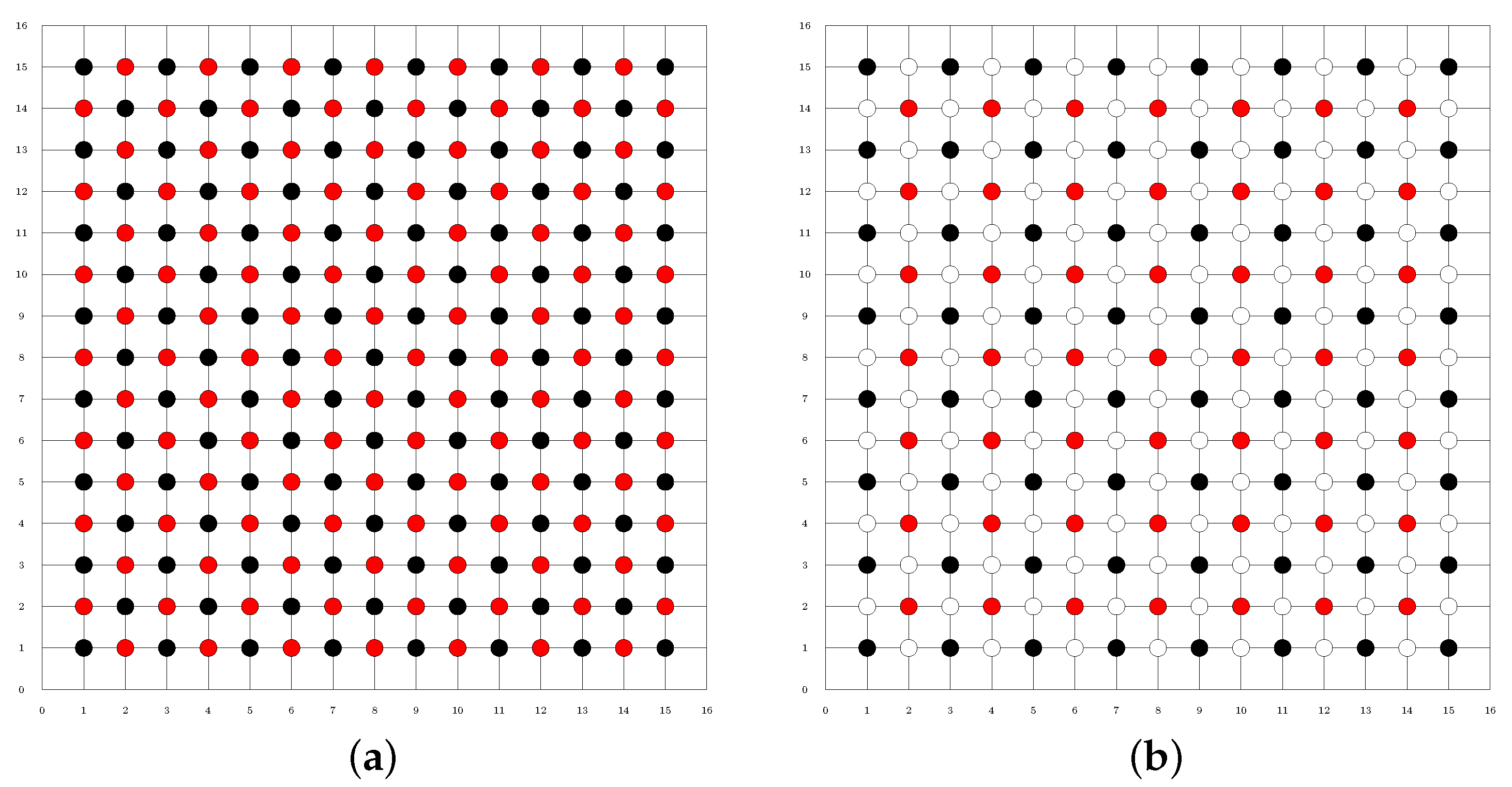
With the AM method, all nodes are involved in the computation, as shown in Figure 3a. The weighted parameter $\omega$ is utilised so that an optimal convergence rate can be obtained by carefully choosing a good value in the range between 1 and 2. Note that in Level 1, the iteration continues from lower node to upper node, while in Level 2, the iteration is carried out in reverse order. Level 3 computes the average sum of the updated values of $u^{\left(1\right)}$ and $u^{\left(2\right)}$ obtained from Levels 1 and 2, respectively. The updating process is repeated until the error rate $ϵ$ satisfies the specified maximum tolerance value.

The SkAM method utilises a skewed grid where computational nodes are equally divided by half into black and white colors; see Figure 3b. The following condition is applied in the computation process so that only black nodes are involved during the iteration procedure:

if (i+j) mod 2 is equal to 0 then

    Update u at point $(i,j)$ for iteration k

else

    Continue

end if

By using the above condition, all white nodes are ignored in the loop of the SkAM algorithm.

3.1. Red–Black Modified AM (MAM) Method

The MAM method employs two different weighted parameters, ${\alpha }_r$ and ${\alpha }_b$, for the respective red and black nodes, and is defined as

$$\left.\begin{array}{cc}\hfill D{\widehat{u}}^{\left(1\right)}& ={\alpha }_c(L{\widehat{u}}^{\left(1\right)}+T{\widehat{u}}^{\left(1\right)})+(1-{\alpha }_c)D{u}^{\left(k\right)}+{\alpha }_{c}f,\hfill \\ \hfill D{\widehat{u}}^{\left(2\right)}& ={\alpha }_c(L{\widehat{u}}^{\left(2\right)}+T{\widehat{u}}^{\left(2\right)})+(1-{\alpha }_c)D{u}^{\left(k\right)}+{\alpha }_{c}f,\hfill \\ \hfill u^{(k+1)}& =\frac{1}{2}\left({\widehat{u}}^{\left(1\right)}+{\widehat{u}}^{\left(2\right)}\right),\hfill \end{array}\right\}$$

(17)

where $c=\{r,b\}$, and ${\alpha }_r$ and ${\alpha }_b$ are the weighted parameters, for the red and black nodes, respectively. The optimal values of the relaxation parameters are in the range $1<{\alpha }_r,{\alpha }_b<2$. It is worth noting that if ${\alpha }_r={\alpha }_b=1$, we will obtain the standard Gauss–Seidel scheme.

All nodes are computed for the MAM method, where red and black nodes are computed in alternating order, as further explained in Section 3.2. The weighted parameters ${\alpha }_1$ and ${\alpha }_2$ are used for red and black iterations, respectively, to achieve the best convergence rate by carefully selecting good values in the range of 1 to 2. It is worth noting that in Level 1, iteration proceeds from lower to upper node, whereas in Level 2, iteration proceeds in the other direction. Level 3 computes the average of the total of the updated ${\widehat{u}}^{\left(1\right)}$ and ${\widehat{u}}^{\left(2\right)}$ values obtained from Levels 1 and 2. The procedure of updating is continued until the error rate $ϵ$ meets the maximum tolerance value.

The SkMAM method is implemented on the skewed grid, where only red and black nodes are involved in the computations. Since the red and black nodes represent 50% of the total nodes in the grid, the computation is reduced approximately by half. All white nodes are ignored during the iteration process.

3.2. Red–Black Ordering

The MAM and SkMAM methods employ red–black ordering, as depicted in Figure 4, where the computational nodes are divided into red and black nodes. For the regular grid applied in the MAM method, half of the nodes are in red color and the other half are in black color. In the case of a skewed grid used for the SkMAM method, half of the nodes are in white color, 25% are red nodes and the remaining 25% are black nodes.

With the red–black strategy, two different weighted parameters, ${\alpha }_1$ and ${\alpha }_2$, are applied to substitute parameter $\omega$ for the respective red and black nodes. Additionally, the accelerated parameter r is replaced with two distinct accelerated parameters, ${\beta }_1$ and ${\beta }_2$. By providing a wider choice of values in the range between 1 and 2 and with appropriate parameter values, this procedure will result in an acceptable optimum number of iterations, and thus speed up the computational time. It can be observed clearly in Figure 5 that the computational molecules for red and black nodes are symmetrical, where the black node applies the updated values of its four neighbouring red nodes and vice versa.

By utilising the red–black ordering approach, red and black nodes are computed alternately. One iteration will involve red nodes only, while in the next iteration, only black nodes are computed. For a skewed grid, all white nodes are ignored during the iterations. These white nodes are only computed once after the convergence is achieved.

4. Red–Black Modified Accelerated Arithmetic Mean (MAAM) Method

The formulation of the proposed two-stage MAAM method also employs a red–black strategy, so an independent equation is applied for the red and black nodes. Unlike the MAM method, which employs weighted parameters only, additional accelerated parameters are utilised for this newly proposed method. It can be constructed based on the AOR iterative scheme (15) to solve the given problem and is written as

$$\left.\begin{array}{cc}\hfill D{\widehat{u}}^{\left(1\right)}& ={\alpha }_c(L+T)u^{\left(k\right)}+(1-{\alpha }_c)D{u}^{\left(k\right)}+{\alpha }_{c}f+{\beta }_d(L({\widehat{u}}^{\left(1\right)}-u^{\left(k\right)})+T({\widehat{u}}^{\left(1\right)}-u^{\left(k\right)})),\hfill \\ \hfill D{\widehat{u}}^{\left(2\right)}& ={\alpha }_c(L+T)u^{\left(k\right)}+(1-{\alpha }_c)D{u}^{\left(k\right)}+{\alpha }_{c}f+{\beta }_d(L({\widehat{u}}^{\left(2\right)}-u^{\left(k\right)})+T({\widehat{u}}^{\left(2\right)}-u^{\left(k\right)})),\hfill \\ \hfill u^{(k+1)}& =\frac{1}{2}\left({\widehat{u}}^{\left(1\right)}+{\widehat{u}}^{\left(2\right)}\right),\hfill \end{array}\right\}$$

(18)

where $c=\{r,b\}$, $d=\{1,2\}$, and ${\alpha }_r$ and ${\alpha }_b$ are the weighted parameters, for the respective red and black nodes, and the constant values ${\beta }_1$ and ${\beta }_2$ are the accelerated parameters at their corresponding Levels 1 and 2. The optimal values for all parameters are in the range $1<{\alpha }_r,{\alpha }_b,{\beta }_1,{\beta }_2<2$. If ${\alpha }_r={\alpha }_b={\beta }_1={\beta }_2$, the original AM method is obtained. Moreover, if ${\alpha }_r={\alpha }_b={\beta }_1={\beta }_2=1$, we obtain the standard Gauss–Seidel method. A proof identical to that given above for Theorem 1 guarantees that the iterative method (18) is convergent for $0<{\alpha }_r,{\alpha }_b,{\beta }_1,{\beta }_2<2$.

The iterative schemes for the MAAM are based on Equation (9), and are written as

$$\begin{array}{cc}\hfill u_{i,j}^{\left(d\right)}=& \frac{{\alpha }_r}{4}\left(u_{i-1,j}^{\left(k\right)}+u_{i+1,j}^{\left(k\right)}+u_{i,j-1}^{\left(k\right)}+u_{i,j+1}^{\left(k\right)}-h^2{f}_{i,j}\right)+(1-{\alpha }_r)u_{i,j}^{\left(k\right)}\hfill \end{array}$$

(19)

and

$$\begin{array}{cc}\hfill u_{i,j}^{\left(d\right)}=& \frac{{\alpha }_b}{4}\left(u_{i-1,j}^{\left(k\right)}+u_{i+1,j}^{\left(k\right)}+u_{i,j-1}^{\left(k\right)}+u_{i,j+1}^{\left(k\right)}-h^2{f}_{i,j}\right)+(1-{\alpha }_b)u_{i,j}^{\left(k\right)}+\hfill \\ \hfill & \frac{{\beta }_d}{4}\left(u_{i-1,j}^{\left(d\right)}-u_{i-1,j}^{\left(k\right)}+u_{i+1,j}^{\left(d\right)}-u_{i+1,j}^{\left(k\right)}+u_{i,j-1}^{\left(d\right)}-u_{i,j-1}^{\left(k\right)}+u_{i,j+1}^{\left(d\right)}-u_{i,j+1}^{\left(k\right)}\right),\hfill \end{array}$$

(20)

for the respective red and black nodes, where d denotes Level 1 or 2. Note that Equation (19) is simply a weighted Jacobi scheme, since it uses the previous values of black nodes. In contrast, Equation (20) utilises the updated values obtained from the prior procedure that computes all red nodes.

Likewise, based on Equation (10), the iterative schemes for the SkMAAM method can be obtained and are written as

$$\begin{array}{cc}\hfill u_{i,j}^{\left(d\right)}=& \frac{{\alpha }_r}{4}\left(u_{i-1,j-1}^{\left(k\right)}+u_{i+1,j-1}^{\left(k\right)}+u_{i-1,j+1}^{\left(k\right)}+u_{i+1,j+1}^{\left(k\right)}-2h^2{f}_{i,j}\right)+(1-{\alpha }_r)u_{i,j}^{\left(k\right)}\hfill \end{array}$$

(21)

and

$$\begin{array}{cc}& u_{i,j}^{\left(d\right)}=\frac{{\alpha }_b}{4}\left(u_{i-1,j-1}^{\left(k\right)}+u_{i+1,j-1}^{\left(k\right)}+u_{i-1,j+1}^{\left(k\right)}+u_{i+1,j+1}^{\left(k\right)}-2h^2{f}_{i,j}\right)+(1-{\alpha }_b)u_{i,j}^{\left(k\right)}+\hfill \\ & \frac{{\beta }_d}{4}\left(u_{i-1,j-1}^{\left(d\right)}-u_{i-1,j-1}^{\left(k\right)}+u_{i+1,j-1}^{\left(d\right)}-u_{d,j-1}^{\left(k\right)}+u_{i-1,j+1}^{\left(d\right)}-u_{i-1,j+1}^{\left(k\right)}+u_{i+1,j+1}^{\left(d\right)}-u_{i+1,j+1}^{\left(k\right)}\right),\hfill \end{array}$$

(22)

for the corresponding red and black nodes, where d is Level 1 or 2.

By using the iterative schemes given in Equations (19)–(22), the corresponding implementations of the MAAM and SkMAAM methods are described in Algorithms 1 and 2, respectively.

Algorithm 1: Modified Accelerated Arithmetic Mean (MAAM)

1: $k=0$ 2: repeat 3:    Level 1: 4:        Compute all red nodes $u_{i,j}^{\left(1\right)}$ using Equation (19) with $c=r,d=1$ 5:        Compute all black nodes $u_{i,j}^{\left(1\right)}$ using Equation (20) with $c=b,d=1$ 6:    Level 2: 7:        Compute all red nodes $u_{i,j}^{\left(2\right)}$ using Equation (19) with $c=r,d=2$ 8:        Compute all black nodes $u_{i,j}^{\left(2\right)}$ using Equation (20) with $c=b,d=2$ 9:    Level 3: 10:        Compute all nodes 11:         $u_{i,j}^{(k+1)}=\frac{1}{2}\left(u_{i,j}^{\left(1\right)}+u_{i,j}^{\left(2\right)}\right)$ 12:    $k=k+1$ 13: until $\left|\right|u_{i,j}^{(k+1)}-u_{i,j}^{\left(k\right)}\left|\right|<ϵ$

As described in the above MAAM algorithm, all nodes are involved during the iteration procedure, in which parameters ${\alpha }_r$, ${\alpha }_b$, ${\beta }_1$ and ${\beta }_2$ are used to optimise the convergence rate, and $ϵ$ is the tolerance error rate. In practice, the optimal values of these parameters are often very close to each other, in which when ${\beta }_2\ge {\beta }_1\ge {\alpha }_b\ge {\alpha }_r$, the convergence is usually found slightly faster.

Algorithm 2: Skewed Modified Accelerated Arithmetic Mean (SkMAAM)

1: $k=0$ 2: repeat 3:    Level 1: 4:        Compute all red nodes $u_{i,j}^{\left(1\right)}$ using Equation (21) with $c=r,d=1$ 5:        Compute all black nodes $u_{i,j}^{\left(1\right)}$ using Equation (22) with $c=b,d=1$ 6:    Level 2: 7:        Compute all red nodes $u_{i,j}^{\left(2\right)}$ using Equation (21) with $c=r,d=2$ 8:        Compute all black nodes $u_{i,j}^{\left(2\right)}$ using Equation (22) with $c=b,d=2$ 9:    Level 3: 10:        Compute all red and black nodes 11:         $u_{i,j}^{(k+1)}=\frac{1}{2}\left(u_{i,j}^{\left(1\right)}+u_{i,j}^{\left(2\right)}\right)$ 12:    $k=k+1$ 13: until $\left|\right|u_{i,j}^{(k+1)}-u_{i,j}^{\left(k\right)}\left|\right|<ϵ$ 14: Compute all white nodes using Equation (5)

Similar to the SkMAM algorithm, only black nodes are computed in the above SkMAAM algorithm. As described above, parameters ${\alpha }_r$, ${\alpha }_b$, ${\beta }_1$ and ${\beta }_2$ are applied to obtain the optimal convergence rate. By checking if $(i+j)$ obtains an even value, all white nodes are ignored during the iteration procedure. Once the maximum error $ϵ$ converges to the specified tolerance value, the remaining white nodes are computed using the standard Formula (5).

5. Numerical Results

In this section, we present some numerical examples in order to compare the considered iterative methods that were described in the previous sections. For simplicity, the iterative methods were applied to Laplace’s equation,

$${\nabla }^{2}u=\frac{{\partial }^{2}u}{\partial x^2}+\frac{{\partial }^{2}u}{\partial y^2}=0,(x,y)\in \mathrm{\Omega }$$

(23)

and the Dirichlet boundary conditions

$$u(x,0)=0.1,u(x,m)=1.0,u(0,y)=0.1,(m,y)=1.0,$$

(24)

where $0\le x\le m$, $0\le y\le m$, and $m=N-1$. These conditions are applied to an $N\times N$ square rectangle computational grid. The experiments were conducted on a Linux machine equipped with an Intel i5-3570K CPU at 3.40 GHz and 8 GB memory.

5.1. Experiment 1

Initially, small grid sizes were chosen to examine the behaviour of the AM method, where $N=16,32,48,64,80$ and 96. Different weighted parameter $\omega$ values were tested in the range of $1<\omega <2$. The convergence rate to stop the iteration procedure was $1.0^{-2}\le ϵ\le 1.0^{-6}$. The number of iterations k and maximum error E were recorded. The boundary conditions (24) were applied and initial inner nodes were set to $u(x^{*},y^{*})=0.1$, where $1\le x^{*}\le N-2$ and $1\le y^{*}\le N-2$.

From

Table 1. Performance of AM method in terms of iterations count (k) and maximum error (E). N is the grid size and $\omega$ denotes the weighted parameter.

	$\mathit{\omega }$	1.20		1.70		1.80		1.99
	$\mathbf{ϵ}$	${\mathbf{1.0}}^{-\mathbf{2}}$		${\mathbf{1.0}}^{-\mathbf{4}}$		${\mathbf{1.0}}^{-\mathbf{6}}$		${\mathbf{1.0}}^{-\mathbf{6}}$
$\mathit{N}$		$\mathit{k}$	$\mathit{E}$	$\mathit{k}$	$\mathit{E}$	$\mathit{k}$	$\mathit{E}$	$\mathit{k}$	$\mathit{E}$
16		24	$9.21\times {10}^{-4}$	34	$8.69\times {10}^{-6}$	55	$8.84\times {10}^{-8}$	340	$9.64\times {10}^{-8}$
32		34	$9.87\times {10}^{-4}$	89	$9.77\times {10}^{-6}$	111	$9.42\times {10}^{-8}$	583	$9.77\times {10}^{-8}$
48		35	$9.78\times {10}^{-4}$	164	$9.99\times {10}^{-6}$	210	$9.70\times {10}^{-8}$	679	$9.92\times {10}^{-8}$
64		35	$9.78\times {10}^{-4}$	256	$9.84\times {10}^{-6}$	336	$9.89\times {10}^{-8}$	712	$9.93\times {10}^{-8}$
80		35	$9.78\times {10}^{-4}$	359	$9.98\times {10}^{-6}$	489	$9.95\times {10}^{-8}$	769	$9.66\times {10}^{-8}$
96		35	$9.78\times {10}^{-4}$	473	$9.93\times {10}^{-6}$	668	$9.90\times {10}^{-8}$	768	$9.67\times {10}^{-8}$

, it can be observed that if the required accuracy is low $ϵ=1.0^{-2}$, the iterations count k does not increase even when a larger grid size is used. However, when higher accuracy $ϵ=1.0^{-6}$ is required, the number of iterations k increases very quickly. It should also be noted that the optimal convergence rate is obtained when the tolerance value is in the range of $1.70\le \omega \le 1.80$ since, when $\omega$ is very close to 2, it will result in a very high iterations count. Therefore, these parameter values were then applied in Experiment 2 so that an optimal convergence rate could be obtained with acceptable accuracy of the solutions.

Figure 6 illustrates that for grid size $N=16$, it requires at least $ϵ=0.01$ so that the solutions can be obtained with acceptable accuracy. When larger grid size $N=96$ is used, higher accuracy $ϵ=0.0001$ is required, as shown in Figure 7.

Stability Analysis

We define that the proposed methods are stable if the obtained maximum absolute error becomes smaller as the computation proceeds. In order to observe this behaviour, the AM and MAM methods were tested with several different parameters. The resulting maximum absolute errors obtained from both methods were observed against the number of iterations. It was assumed that the same behaviour would be achieved for the proposed methods.

Figure 8 demonstrates the stability of the AM and MAM methods with several different parameters. It can be seen clearly from the graphs that as the number of iterations increases, the maximum error becomes smaller to achieve the convergence criterion. This stable condition was true for different grid sizes ($N=\{64,128,256,512\}$), several weighted parameter values ($1.4\le \omega \le 1.7,1.2\le {\alpha }_r,{\alpha }_b\le 1.8$) and various tolerance errors ($1.0^{-6}\le ϵ\le 1.0^{-4}$).

5.2. Experiment 2

In the final experiments, the convergence rate was $ϵ=1.0\times {10}^{-7}$, and the chosen values of $\omega$ and r were in the range of between $1.70$ and $1.90$. Sufficient different grid sizes of $N=128,256,384,512,640$ and 768 were chosen to record the iteration counts and execution time of the considered methods.

Table 2. Number of iterations (k) and execution time (t) in seconds of the considered iterative methods. N is the size of grid, ${\alpha }_1$ and ${\alpha }_2$ are the weighted parameters, ${\beta }_1$ and ${\beta }_2$ are the accelerated parameters, and E is the maximum error.

	Methods	N	${\mathit{\alpha }}_1$	${\mathit{\alpha }}_2$	${\mathit{\beta }}_1$	${\mathit{\beta }}_2$	k	t	E
REGULAR MESH	AM	128	1.70	1.70	1.70	1.70	1641	0.83	$9.9836\times {10}^{-8}$
		256	1.71	1.71	1.71	1.71	5312	11.05	$9.9880\times {10}^{-8}$
		384	1.72	1.72	1.72	1.72	10,228	46.55	$9.9965\times {10}^{-8}$
		512	1.73	1.73	1.73	1.73	15,961	135.95	$9.9987\times {10}^{-8}$
		640	1.74	1.74	1.74	1.74	22,214	292.58	$9.9986\times {10}^{-8}$
		768	1.75	1.75	1.75	1.75	28,763	570.83	$9.9999\times {10}^{-8}$
	MAM	128	1.72	1.70	1.72	1.72	1453	0.73	$9.9659\times {10}^{-8}$
		256	1.73	1.71	1.73	1.73	4701	9.41	$9.9999\times {10}^{-8}$
		384	1.74	1.72	1.74	1.74	9037	40.99	$9.9947\times {10}^{-8}$
		512	1.75	1.73	1.75	1.75	14,067	122.14	$9.9988\times {10}^{-8}$
		640	1.76	1.74	1.76	1.76	19,519	255.97	$9.9994\times {10}^{-8}$
		768	1.77	1.75	1.77	1.77	25,186	492.20	$9.9993\times {10}^{-8}$
	MAAM	128	1.72	1.70	1.74	1.80	1116	0.55	$9.9433\times {10}^{-8}$
		256	1.73	1.71	1.75	1.81	3604	7.56	$9.9814\times {10}^{-8}$
		384	1.74	1.72	1.76	1.82	6877	31.47	$9.9943\times {10}^{-8}$
		512	1.75	1.73	1.77	1.83	10,606	91.70	$9.9967\times {10}^{-8}$
		640	1.76	1.74	1.78	1.84	14,554	188.85	$9.9993\times {10}^{-8}$
		768	1.77	1.75	1.79	1.85	18,539	363.39	$9.9977\times {10}^{-8}$
SKEWED MESH	SkAM	128	1.70	1.70	1.70	1.70	885	0.32	$9.9756\times {10}^{-8}$
		256	1.71	1.71	1.71	1.71	2913	4.21	$9.9991\times {10}^{-8}$
		384	1.72	1.72	1.72	1.72	5674	18.54	$9.9892\times {10}^{-8}$
		512	1.73	1.73	1.73	1.73	8936	53.10	$9.9978\times {10}^{-8}$
		640	1.74	1.74	1.74	1.74	12,538	117.61	$9.9961\times {10}^{-8}$
		768	1.75	1.75	1.75	1.75	16,352	222.95	$9.9992\times {10}^{-8}$
	SkMAM	128	1.72	1.70	1.72	1.72	800	0.31	$9.9445\times {10}^{-8}$
		256	1.73	1.71	1.73	1.73	2634	3.81	$9.9707\times {10}^{-8}$
		384	1.74	1.72	1.74	1.74	5120	16.68	$9.9929\times {10}^{-8}$
		512	1.75	1.73	1.75	1.75	8046	48.31	$9.9943\times {10}^{-8}$
		640	1.76	1.74	1.76	1.76	11,258	106.15	$9.9955\times {10}^{-8}$
		768	1.77	1.75	1.77	1.77	14,637	210.31	$9.9968\times {10}^{-8}$
	SkMAAM	128	1.72	1.70	1.74	1.80	691	0.27	$9.9883\times {10}^{-8}$
		256	1.73	1.71	1.75	1.81	2276	3.56	$9.9751\times {10}^{-8}$
		384	1.74	1.72	1.76	1.82	4409	15.60	$9.9919\times {10}^{-8}$
		512	1.75	1.73	1.77	1.83	6896	42.77	$9.9993\times {10}^{-8}$
		640	1.76	1.74	1.78	1.84	9597	95.11	$9.9937\times {10}^{-8}$
		768	1.77	1.75	1.79	1.85	12,398	168.90	$9.9991\times {10}^{-8}$

shows that the proposed MAAM outperforms the existing AM and MAM methods in terms of iterations and execution time. Moreover, the skewed variants clearly outperform their conventional counterparts, with the SkMAAM method providing the greatest results. The MAAM and SkMAAM methods are also more flexible than the previous AM, MAM, SkAM and SkMAM methods, because they include additional accelerated parameters, allowing for a greater range of parameter values. As shown in the maximum error value, all methods achieve an acceptable tolerance rate in terms of accuracy.

Table 3. Average reduction percentage in terms of iterations count and execution time.

METHODS	Iterations Reduction	Time Reduction
MAM vs. AM	11.84%	12.55%
MAAM vs. AM	33.41%	33.68%
MAAM vs. MAM	24.48%	24.14%
SkAM vs. AM	44.41%	60.87%
SkMAM vs. MAM	43.21%	58.77%
SkMAAM vs. MAAM	35.50%	51.79%
SkMAM vs. SkAM	9.93%	7.85%
SkMAAM vs. SkAM	22.76%	18.29%
SkMAAM vs. SkMAM	14.24%	11.25%

shows the reduction percentages in terms of iterations and time. The MAM method performs better than the AM method. In comparison to the AM and MAM methods, the suggested MAAM method decreases iterations and execution time by roughly 33% and 24%, respectively. The skewed methods reduce iterations and execution time by 34% to 44% and 52% to 61%, respectively, when compared to their standard variants. Meanwhile, the improved SkMAAM method has a reduced iteration count and execution time compared to the SkMAAM method by around 14% and 11%, respectively. The SkMAAM is also clearly better than the SkAM method by providing much lower iteration counts and execution time.

Figure 9 shows the comparison between the considered methods in terms of the number of iterations, where the skewed variants (shown in solid lines) require a lower number of iterations compared to their corresponding standard variants (dashed lines). Meanwhile, Figure 10 illustrates the execution time of the considered iterative methods, in which the SkMAAM method has consistently outperformed the other methods. It is also shown that the execution time increases rapidly compared to the size of the grid. The graph shows that the iterations of all methods grow almost linearly with the increase in grid size.

6. Discussion

Only one weighted value is used as a relaxation parameter to speed up the computation for the existing AM and its skewed SkAM variant. For the modified variants of the MAM and MAAM methods and their corresponding skewed methods, two different weighted values are applied for red and black nodes, respectively. Meanwhile, the proposed MAAM and its skewed variant also apply an additional two distinct accelerated parameters. As a result, there is a greater variety of parameter tuning options available. When good parameter values are chosen, as shown in the numerical experiment findings, the MAAM variants execute quicker than the existing AM and MAM variants.

All skewed variants, SkAM, SkMAM and SkMAAM, outperform their corresponding regular variants since they only consider half of the total nodes. Only red and black nodes are computed in the iteration process when using a skewed grid. After the convergence requirement is met, the remaining white nodes are computed only once. The skewed variants lower the number of iterations and execution time by half in terms of computational complexity. In terms of accuracy, all methods achieve an acceptable maximum error rate.

Computation at Level 1 begins by computing all red nodes. After that, all black nodes are computed, in which each black node utilises the updated red nodes. Similarly, at Level 2, the process begins by computing all red nodes and is followed by the computation of all black nodes. Finally, the average of the updated values obtained from Levels 1 and 2 is computed at Level 3. As a result, since these methods require two independent computations that may be performed in parallel, their parallel versions should outperform their sequential implementations. The application of the red–black strategy allows each red node to be computed concurrently and vice versa. Therefore, the computation of red and black nodes can be carried out in alternating order, where the parallel algorithms can be implemented easily. Furthermore, the availability of a fast and affordable Graphical Processing Unit (GPU) makes such parallel implementation very attractive. The suggested improved accelerated two-stage iterative methods with red–black ordering can also be applied to solve other types of partial differential equations.

Although additional parameters provide a wider choice of options, they pose a challenge in finding good optimum values. Since there is no formula currently available to immediately give the optimum value, several trial runs have to be conducted to study the response of the AM method to the chosen parameters, as explained in Experiment 1. It is assumed that the good optimum values found for the AM method are also valid for the other methods since their iterative schemes are all derived from the same finite difference approximation equations.

7. Conclusions

All of the methods investigated in this study have two levels of computations, each of which is totally independent, making them ideal for parallel implementation. As a result, such a parallel solution should greatly reduce the execution time. In addition to the existing relaxation parameter in the AM and SkAM, the use of two weighted parameters provides different relaxation values for red and black nodes applied in the MAM, SkMAM, MAAM and SkMAAM methods. The introduction of two accelerated parameters to the respective red and black nodes further improves the overall performance of the newly proposed MAAM and SkMAAM methods.

The computational complexity of the iterative method implemented on the skewed grid can be decreased by around half by using the half-sweep iteration procedure. Because only half of the total nodes in the computational grid are considered throughout the iteration process, the skewed variant implemented using the half-sweep technique outperforms the regular variant constructed using the full-sweep technique on a regular grid. We plan to look into parallel implementations of the proposed methods in future work. More advanced approaches such as a quarter-sweep technique and implementation on a block grid would be examined. The potential application of the proposed methods for solving fractional-order partial differential equations in the extended work is seriously considered.

References

- Evans, D.J.; Sahimi, M.S. The alternating group explicit (age) iterative method for solving parabolic equations i: 2-dimensional problems. Int. J. Comput. Math. 1988, 24, 311–341. [Google Scholar] [CrossRef]
- Galligani, I.; Ruggiero, V. The arithmetic mean method for solving essentially positive systems on a vector computer. Int. J. Comput. Math. 1990, 32, 113–121. [Google Scholar] [CrossRef]
- Muthuvalu, M.S.; Galligani, E.; Ali, M.K.M.; Sulaiman, J.; Lebelo, R.S. Performance analysis of Arithmetic Mean method for solving composite 6-point closed Newton–Cotes quadrature algebraic equation. Asian-Eur. J. Math. 2019, 12, 1950061. [Google Scholar] [CrossRef]
- Sahimi, M.S.; Khatim, M. The Reduced Iterative Alternating Decomposition Explicit (RIADE) method for the diffusion equation. Pertanika J. Sci. Tech. 2001, 9, 13–20. [Google Scholar] [CrossRef]
- Hussain, A.; Muthuvalu, M.S.; Faye, I.; Ali, M.K.M.; Lebelo, R.S. Numerical Study of Glioma Growth Model with Treatment Using the Two-Stage Gauss-Seidel Method. J. Phys. Conf. Ser. 2018, 1123, 012040. [Google Scholar] [CrossRef]
- Sulaiman, J.; Othman, M.; Hasan, M.K. A new Half-Sweep Arithmetic Mean (HSAM) algorithm for two-point boundary value problems. In Proceedings of the International Conference on Statistics and Mathematics and Its Application in the Development of Science and Technology, Bandung, Indonesia, 4–6 October 2004; pp. 169–173. [Google Scholar]
- Young, D.M. Iterative Solution of Large Linear Systems; Academic Press: Cambridge, MA, USA, 1971. [Google Scholar]
- Saad, Y.; van der Vorst, H.A. Iterative solution of linear systems in the 20th century. J. Comput. Appl. Math. 2000, 123, 1–33. [Google Scholar] [CrossRef] [Green Version]
- Hong, E.J.; Saudi, A.; Sulaiman, J. Numerical Evaluation of Quarter-Sweep SOR Iteration for Solving Poisson Image Blending Problem. In Proceedings of the 2018 IEEE International Conference on Artificial Intelligence in Engineering and Technology (IICAIET), Kota Kinabalu, Malaysia, 8 November 2018; pp. 1–5. [Google Scholar] [CrossRef]
- Musli, F.A.; Saudi, A. Agent Navigation via Harmonic Potentials with Half-Sweep Kaudd Successive over Relaxation (HSKSOR) Method. In Proceedings of the 2019 IEEE 9th Symposium on Computer Applications Industrial Electronics (ISCAIE), Kota Kinabalu, Malaysia, 27–28 April 2019; pp. 335–339. [Google Scholar] [CrossRef]
- Hadjidimos, A. Accelerated overrelaxation method. Math. Comput. 1978, 32, 149–157. [Google Scholar] [CrossRef]
- Sunarto, A.; Agarwal, P.; Sulaiman, J.; Chew, J.V.L.; Aruchunan, E. Iterative method for solving one-dimensional fractional mathematical physics model via quarter-sweep and PAOR. Adv. Differ. Equ. 2021, 2021, 147. [Google Scholar] [CrossRef]
- Huang, Z.G.; Cui, J.J. Accelerated Relaxation Modulus-Based Matrix Splitting Iteration Method for Linear Complementarity Problems. Bull. Malays. Math. Sci. Soc. 2021, 44, 2175–2213. [Google Scholar] [CrossRef]
- Dahalan, A.; Saudi, A.; Sulaiman, J. Autonomous navigation on modified AOR iterative method in static indoor environment. J. Phys. Conf. Ser. 2019, 1366, 012020. [Google Scholar] [CrossRef]
- Li, R.; Gong, L.; Xu, M. A heterogeneous parallel Red-Black SOR technique and the numerical study on SIMPLE. J. Supercomput. 2020, 76, 9585–9608. [Google Scholar] [CrossRef]
- Ali, U.; Abdullah, F.A. Modified implicit difference method for one-dimensional fractional wave equation. AIP Conf. Proc. 2019, 2184, 060021. [Google Scholar] [CrossRef]
- Singh, J.; Ahmadian, A.; Rathore, S.; Kumar, D.; Baleanu, D.; Salimi, M.; Salahshour, S. An efficient computational approach for local fractional Poisson equation in fractal media. Numer. Methods Partial Differ. Equ. 2021, 37, 1439–1448. [Google Scholar] [CrossRef]
- Saudi, A.; Sulaiman, J. Half-Sweep Arithmetic Mean Method for Solving 2D Elliptic Equation. Int. J. Appl. Math. Stat. 2019, 58, 52–59. [Google Scholar]
- Saudi, A.; Sulaiman, J. An Efficient Two-Stage Half-Sweep Modified Arithmetic Mean (HSMAM) Method for the Solution of 2D Elliptic Equation. Adv. Sci. Lett. 2018, 24, 1417–1921. [Google Scholar] [CrossRef]
- Abdullah, A.R. The four point Explicit Decoupled Group (EDG) method: A fast Poisson solver. Int. J. Comput. Math. 1991, 38, 61–70. [Google Scholar] [CrossRef]
- Ruggiero, V.; Galligani, E. An iterative method for large sparse linear systems on a vector computer. Comput. Math. Appl. 1990, 20, 25–28. [Google Scholar] [CrossRef] [Green Version]
Figure 1.
Portion of regular computational grid about point for AM method at (a) Level 1 and (b) Level 2.
Figure 2.
Portion of skewed computational grid about point for SkAM method at (a) Level 1 and (b) Level 2.
Figure 3.
The standard computational mesh of (a) regular and (b) skewed cases for the AM and SkAM methods, respectively.
Figure 4.
The red–black computational mesh for (a) regular and (b) skewed cases.
Figure 5.
The computational molecules for finite difference approximation of regular (left a,b) and skewed (right c,d) cases. The molecules of red and black nodes are symmetrical for both cases, in which the black node applies the updated values of its four neighbouring red nodes and vice versa.
Figure 6.
Solution of Laplace’s equation using different maximum error rate and grid size . Graphs (a,b) give lower accuracy, whereas (c,d) illustrate the solutions that require toobtain acceptable accuracy.
Figure 7.
Solution of Laplace’s equation for grid size with different maximum error rate. Acceptable accuracy is obtained when . (a) ; (b) ; (c) ; (d) .
Figure 8.
As the computation proceeds, the maximum errors become smaller. (a) ; (b) ; (c) ; (d) ; (e) ; (f) ; (g) ; (h) .
Figure 9.
The number of iterations for the considered iterative methods.
Figure 10.
The execution time of the considered iterative methods.