Fast Shape Recognition via the Restraint Reduction of Bone Point Segment

Abstract

In computer science, and especially in computer vision, the contour of an object is used to describe its features; thus, the shape descriptor plays an indispensable role in target detection and recognition. Further, Fourier is an important mathematical description method, and the Fourier transform of a shape contour has symmetry. This paper will demonstrate the symmetry of shape contour in the frequency domain. In recent years, increasing numbers of shape descriptors have come to the fore, but many descriptors ignore the details of shape. It is found that the most fundamental reason affecting the performance of shape descriptors is structural restraints, especially feature structure restraint. Therefore, in this paper, the restraint of feature structure that intrinsically deteriorates recognition performance is shown, and a fast shape recognition method via the Bone Point Segment (BPS) restraint reduction is proposed. An approach using the inner distance to find bone shapes and segment the shape contour by these bones is proposed. Then, Fourier transform is performed on each segment to form the shape feature. Finally, the restraints of the shape feature are reduced in order to build a more effective shape feature. What is commendable is that its discriminability and robustness is strong, the process is simple, and matching speed is fast. More importantly, the experiment results show that the shape descriptor has higher recognition accuracy and the matching speed runs up to more than 1000 times faster than the existing description methods like CBW and TCD. More importantly, it is worth noting that the recognition accuracy approaches 100% in the self-build dataset.

1. Introduction

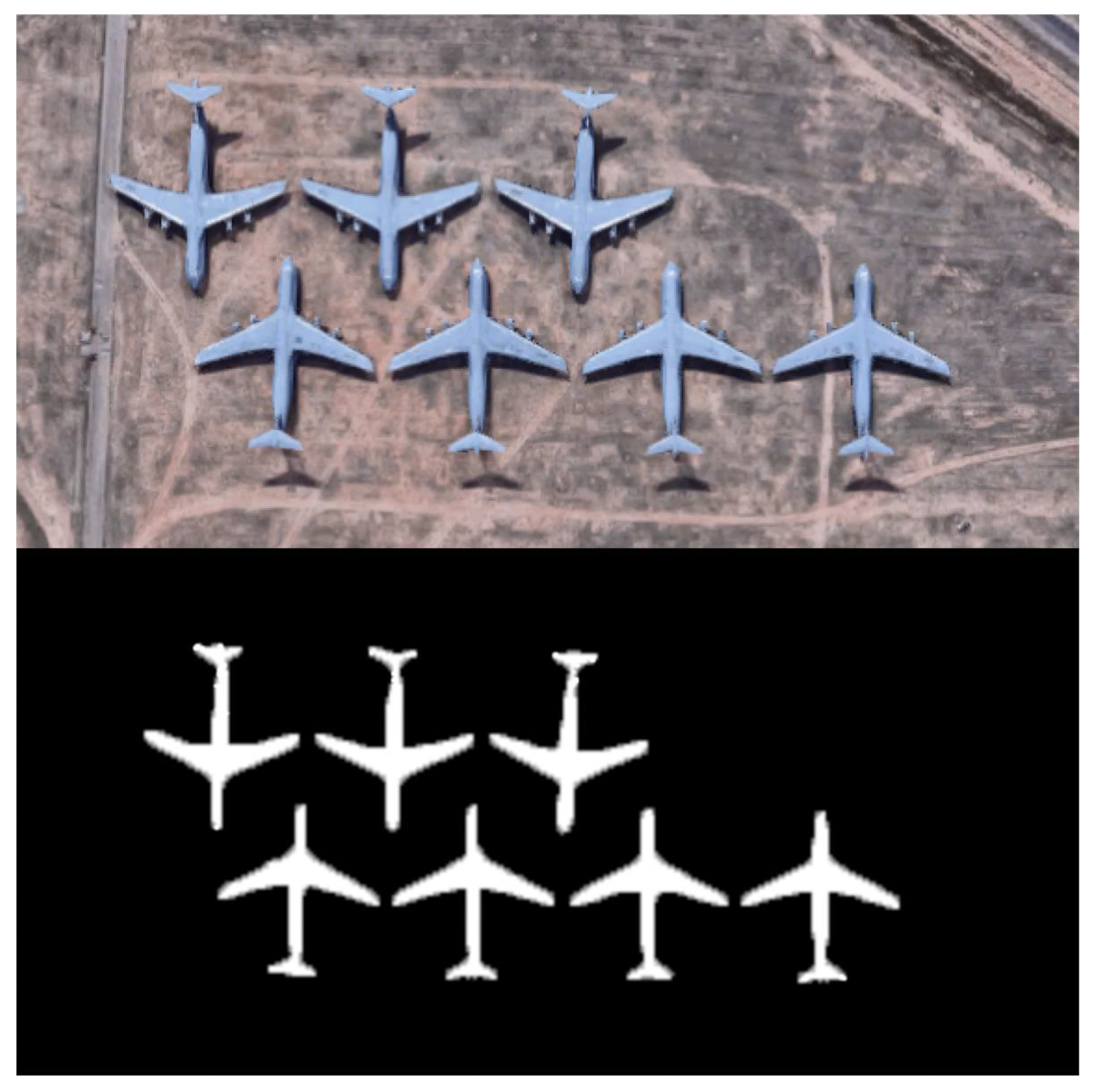
With the continuous progress of computer vision, researchers are increasingly studying sensors and remote sensing image information, including a substantial number of articles describing image features, particularly shape features. Shape descriptors play an important role in object recognition and detection, they are also universally used in remote image processing and analyzing, remote sensing measurement, and machine vision. When the object in the whole image is too small or the shape of the object is variable, the shape descriptor can be used to describe the object by extracting shape features, where the shape feature and object feature are the same, as shown in Figure 1.

Figure 1. The upper half is a remote sensing image for warcrafts and the lower half shows the shapes of the objects in the upper. As clearly shown in the figure, shape plays an important role in remote sensing image detection and recognition.

Many shape descriptors have been proposed [1,2,3,4,5]. They can be roughly divided into three clalsses: global descriptors, local descriptors, and syncretic descriptors. They can also be divided into shape descriptors in the spatial domain and shape descriptors in the frequency domain. Global descriptors can represent the overall features of the shape, but might miss the details of the shape. Local descriptors describe the features in more detail, but may only partially display the feature. The spatial domain descriptor describes features that are more visible, and easy to understand. However, although the frequency domain descriptor represents a more abstract feature, it is more robust.

Shape descriptors are used to extract shape features of objects [6,7]. Some well known shape descriptors include FD (Fourier descriptor) [8], CCD (centroid contour distance), FD-CCD (CCD based FD) [8], FPD (farthest point distance) [9], WD (wavelet descriptor) [10], SC (shape context) [3]. There are also some improved descriptors, such as FMSCCD (Fourier descriptor based on multi-scale centroid distance) [11], IDSC (shape context based on inner distance) [12], and ASD & CCD (angular scale descriptor based on distance from centroid) [13]. The ability of a shape descriptor is evaluated mainly by translating, rotating, and scaling the shape to see whether it can still correctly distinguish. A shape descriptor must satisfy translation, rotation, and scale invariance.

FD [13] is a representative frequency domain descriptor, which has the potential of practical application due to its excellent stability and balance in feature performance. Usually, FD first obtains the spatial domain vectors of features and then converts them into frequency domain vectors. For example, in the FD-CCD method, the shape CCD feature vector is first calculated and then transformed into the frequency domain to construct the FD-CCD shape descriptor. Because the CCD method cannot guarantee a consistent starting point of feature. But for FD-CCD, authors don’t have to worry about the starting point after taking the Fourier transform of the feature, which can reduce the matching time and increase the accuracy of the result.

Generally, the Fourier method [14] based on contour points calculates the area where other contour points are relative to a given contour point in the frequency domain. However, there is a common problem with FD, in that it fuses local features to form global features. In this way, the deformation of local contour will greatly affect the Fourier feature, and then affect the shape recognition result. Traditional target recognition methods based on Fourier transform mostly focus on recognition accuracy and precision. Due to the low speed, it becomes an application bottleneck. The essential problem is the existence of “structural restraints”. Moreover, the research method for this paper focuses on the structural restraints of features in shape recognition.

Recently, deep learning-based methods [15,16,17] and neural network-based methods [4,18,19] exhibit outstanding performance in object detection and recognition after data training. However, practicability is restricted by two major factors, some image data sets are difficult to obtain, and existing public datasets are generally small. Therefore, feature-based shape description is particularly important. On the other hand, rather than conventional methods, Bicego and Lovato [20] proposed the biogenic informatics model to achieve two-dimensional shape recognition. The key idea is to code the shape contour into biological information sequences according to its spatial distribution, i.e., DNA molecular sequences, and then adopt some chain code-matching calculation methods to analyze the similarity between sequences, thus achieving shape recognition and classification.

So, in this paper, we proposed Fast shape recognition via Bone Points Segment (BPS) restraint reduction. First, the inner distance is used to find the bone points of the shape contour, then segment the contour by the bone points and put all the segmented contour parts on the same coordinate axis. Second, Fourier transform is performed on each respective contour segment. Finally, the reduction restraint is applied on the Fourier feature, and in this way, heavily deformed contour segments can be removed. In the matching stage, the final accuracy of shape recognition is obtained by the Fourier feature based on BPS, which provides considerable performance compared with other state-of-the-art methods in shape recognition.

The author’s contributions in this paper include:

(1)

The author proposes a new method for contour segmentation based on bone points using inner distance;

(2)

The author introduces a new concept of “structural restraint” in shape recognition;

(3)

The author exhibits a new framework of shape Fourier feature and the reduction restraint is applied into this feature.

The rest of the paper begins with the following. In the second part, the new concepts and research work related to Fourier shape recognition with reducing the restraint of feature are introduced, including the definition and description of some new concepts, the inner distance based on shape contour points, and the advantages and disadvantages of shape descriptors based on Fourier transform. The third part describes the relevant research ideas and work of the proposed method, and explains the model of the proposed shape recognition method in detail. The fourth part is the experimental part. The proposed method is tested in the small dataset and compared with the results of other existing shape recognition methods in three international mainstream general databases. At the same time, the results of the proposed method are compared with those of the method without the reduction constraint. Finally, the conclusions, prospects, and acknowledgments of the method are presented.

2. Related Work

In this part, we find some essential problems that affect the speed and accuracy of shape recognition, describe the concept and definition of related shape recognition restraints, introduce the advantages of shape distance, and finally introduce the advantages and disadvantages of current representative shape descriptors based on Fourier transform. The shape descriptors obtained by directly extracting all edge contour points from planar shapes are usually of poor stability and robustness, which leads to low matching accuracy of target shape features.

2.1. The Essential Problem of Shape Recognition and Relevant Restraint Concepts

2.1.1. The Essential Problem of Shape Recognition Methods Based on Fourier Transform

Traditional shape matching and recognition methods [21] mostly focus on recognition accuracy and precision. Due to the time consuming and low-speed process [1,22], it becomes an application bottleneck. The essential problem is the existence of “structural restraints”. Moreover, the research method for this paper focuses on the structural restraints of features in shape recognition. The shape descriptors obtained by directly extracting all edge contour point information for flat shapes usually have poor stability, which leads to poor accuracy in matching shape features of the target. In addition, the feature structure of common shape descriptors [23] is too complex and integrated when extracting shape features, resulting in slow recognition speed. The four reasons for the “structural restraint feature” are analyzed as follows:

• The plane image of the target may have strong local deformation, which will cause the global feature of the target to be distorted. The global feature is used to describe that the shape may be completely mismatched in the matching stage;
• As the plane image of the target obtained is changeable and its shape structure are unstable, the shape and feature are changeable and unstable;
• Using overly complex shape features for simple shapes will cause excessive computational effort in the subsequent matching stage;
• For the vast majority of international general databases, the shape degree of shape contour, i.e., the features of contour frequency domain, are different. The shape features with the same restraints may produce different description ability for different databases, thus restricting the overall expression ability of shape descriptors.

2.1.2. Creative Concepts of Relevant Restraints

In mathematics, a restraint is the condition that the solution of an optimization problem needs to meet. When analyzing some specific logic functions, researchers often encounter situations where the value of input variables is not arbitrary. Restrictions on the value of input variables become restraints. Reducing restraints is to change the relevant factors affecting the process and meet a specific result or requirement, that is, the input or output parameters of a process, and reducing the influence these factors will have in terms of a positive effect on the expected results. Similarly, there may be a series of restraints in shape recognition analysis, including restraints generated by extracting shape features, restraints generated in the process of shape feature calculation and restraints generated in the process of shape matching, etc. Here, all factors that affect the accuracy and speed of shape recognition results in the process of shape recognition are collectively referred to as shape recognition restraints. Therefore, in shape recognition, the authors consider the new concept of reducing shape recognition restraints in order to improve the speed and accuracy of shape recognition. In this paper, the concept of “structural restraint”, which is the essential issue affecting the shape recognition result, is proposed for the first time. Besides, the related concepts of parent and child restraints are defined in this section, which include structural restraints and feature structure restraints.

Structural restraints: The process of shape recognition mainly contains three stages: shape feature description, shape feature calculation and shape feature matching. Therefore, a series of restraints affecting the performance (speed and accuracy) of shape recognition in the three stages are defined as structural restraints, which includes feature structure restraint, calculation structure restraint and matching structure restraint.

Feature structure restraint: Feature structure restraint is the parent restraint in the feature description stage of shape recognition. The feature structure restraint is defined as the sub-restraint of the structural restraints which affects the shape recognition performance in the feature description stage.

2.2. Inner Distance

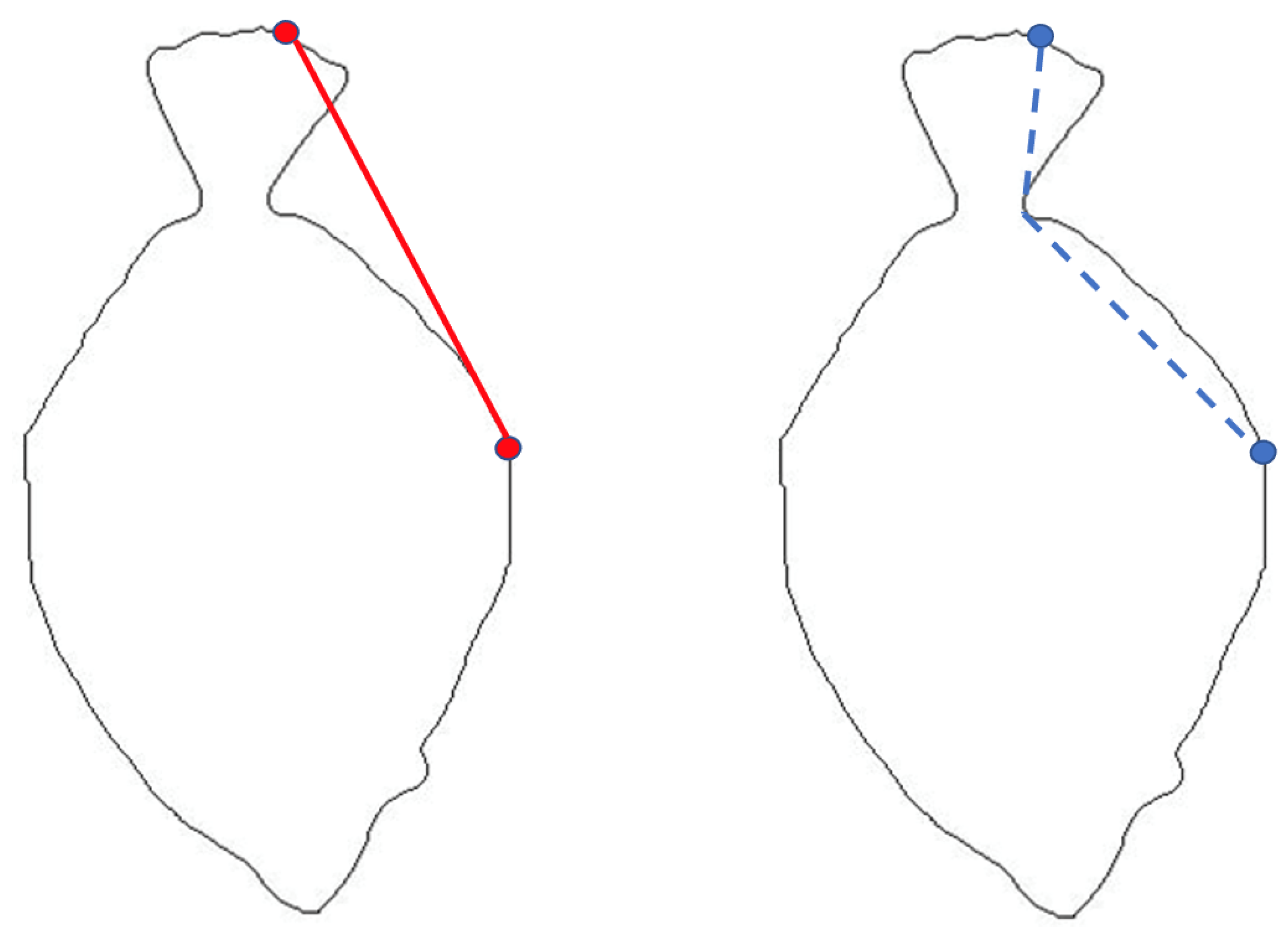
Distance is an important mathematical variable to describe shapes [24]. The distance we generally refer to is called the Euclidean distance, which is the distance of a straight line. The inner distance refers to the polyline distance, which is completely inside the shape contour. The Euclidean and inner distances of two points in the same shape are shown in Figure 2. Obviously, there is a significant difference between the distance AB and the inner distance A’B’ between the two points of this pair of shapes.

Figure 2. Two objects. The left straight line shows the Euclidean distance from A to B, the right polyline shows the inner distance from A’ to B’. It’s clear that the correlation with shape is closer for the inner distance between the two points of the shape but not the Euclidean distance.

For local insensitivity, many researchers believe that the inner distance captures part structures better than the Euclidean distance. For example, Distance Interior Ratio (DIR) [25], Inner Distance Shape Context (IDSC) [12] and Vertical Interior Distance Ratio (VIDR) [26] all use the interior distance for the feature of shapes, and the results verify that those shape features based on the inside of the shape have higher recognition accuracy than the feature based on Euclidean distance. Indeed, the shape feature using the method related to the inner shape can achieve higher accuracy to a great extent.

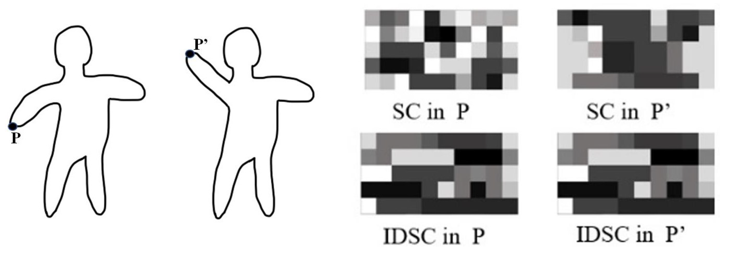
This is hard to prove because the definition of local features remains unclear. However, there is a test for this purpose. For example, Shape Context (SC) [3] is a well-known shape contour descriptor proposed in 2002. It is a global descriptor. The shape context of each point in the contour point set is a circular distribution area, which reveals the spatial relationship of remaining points to the current point, and the shape context of the target is represented by a set of histograms. However, based on the idea of Shape Context, Ling and Jacobs [12] proposed to use IDSC between contour points to replace Belongie et al. [3] in calculating Euclidean Distance adopted in Shape Context. The shortest path length of two sampling points in contour sequence through the inside of the shape is defined as the inner distance. This method is suitable for the identification of the target with flexible change, and good results are achieved in the experiment. Figure 3 gives a shape which is a nonrigid object and shows severe deformation, and for one point, as tested by SC and IDSC. It is clear that the feature of SC is dissimilar, while IDSC is almost similar in the points of P and P’. From this figure, it can see that the inner distance is better at capturing parts than SC. The inner distance is just a byproduct of the shortest path algorithms and does not affect the complexity. So, inner distance has strong robustness to describe shape features. More importantly, the proposed method will use inner distance to find the bone point shapes in Section 3.

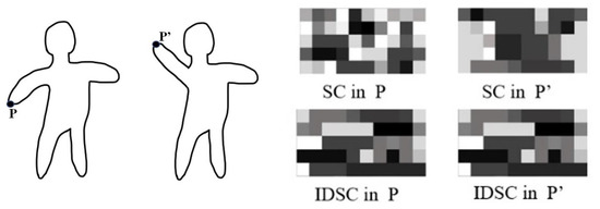
Figure 3. The left side is one pair of shapes with different arm positions. The right side shows the SC and IDSC features of two points P and P’ on the left shapes.

Figure 3 shows the results of the comparison between SC and IDSC, and shows an example where the inner distance distinguishes a pair of the same target while the Euclidean distance encounters problems because the sample points on the shape have the same spatial distribution. For example, the original SC may fail on these shapes. One could argue that Euclidean distance also applies to these examples. There are some practical troubles in this argument. First of all, the computational cost greatly increases, and no matter how many points are used, it can always possess a finer structure. Finally, for some nonrigid objects this strategy will run into trouble. It can be seen from the Figure 3 that inner distance exhibits a great ability to describe shapes.

2.3. Fourier Transform of the Shape

Fourier transform was first systematically proposed by the French mathematician and physicist Fourier in 1807 [27]. It’s a common orthogonal transformation. If the image is described in terms of functions, the orthogonal transformation is the decomposition of a function into a linear combination of orthogonal functions. The idea of Fourier transformation for shapes is the transformation of geometric features from the spatial domain to the frequency domain for processing [28]. The advantages are as follows:

• It has good anti-noise ability and adaptability to analyze shape features in the frequency domain;
• The frequency domain conversion reduces the redundancy of sample space, optimizes the storage space and reduces the computational complexity. Fourier transform plays an important role in feature extraction, shape analysis, and shape recognition.

2.3.1. Fourier Transform of the Shape

For the Fourier transformation of an image, the two-dimensional image is first represented as a one-dimensional contour function shape. On this basis, Fourier transform theory is used to expand it, and the Fourier coefficient is used as a shape descriptor. The essence of Fourier descriptors is to describe contour features by a set of numbers representing the overall frequency components of shapes.

Suppose the contour of an object shape is composed of a series of coordinate pixels $\left(x_i,y_i\right)$ with a total length of N, pixel point $i\in [0,N-1]$. The coordinates $\left(x_0,y_0\right),\left(x_1,y_1\right)$ $\dots ,(x_{(n-1)},y_{(n-1)})$ are the point set that passes clockwise or counterclockwise along the contour, and the sequence formed by the point set is represented as the contour coordinate sequence, which can be expressed as the below Equation (1).

$$f(x,y)=f\left(m\right)=\left[\left(x_0,y_0\right),\left(x_1,y_1\right),\dots ,\left(x_{(n-1)},y_{(n-1)}\right)\right]$$

(1)

where, m represents the coordinate point of the shape contour. Discrete Fourier transform (DFT) not only has definite physical meaning, but is also easy to calculate, and is widely used in digital signal processing system. DFT establishes the “bridge relation” between the discrete time domain and the discrete frequency domain. In essence, the finite point discrete sampling of the finite-length Fourier transform sequence is carried out to discretize the frequency domain, so that image digital signal correlation processing can be carried out in the frequency domain using the digital operation method. Fourier descriptors have the following characteristics: (1) They are a compact descriptor; (2) They can effectively eliminate high-frequency components in image shape information; (3) They are a description method that is easily normalized. Assuming that the two-dimensional shape contour function is $F\left(x\right)$, its discrete Fourier transform can be expressed as the Equation (2).

$$F\left(f\left(x\right)\right)=F\left(m\right)=1/N\sum _{x=0}^{N-1}f\left(x\right)e^{\left((-j2\pi mx)/N\right)},m=0,1,\dots ,N-1$$

(2)

Here, the author put the coefficient $1/N$, which is commonly used in the inverse one-dimensional Discrete Fourier transform, into the forward transform, to ensure that the product of the coefficients before the forward transform and the inverse transform is equal to $1/N$, or that it can multiply the forward transform and the inverse transform by $1/\sqrt{N}$, respectively. A discrete sequence is still a discrete sequence after the Fourier transform. Where each m corresponds to the weighted sum of all the inputs $f\left(x\right)$ after the Fourier transform, and m determines the frequency of the results of each Fourier transform. The fast Fourier Transform (FFT) was proposed in the 1960s to reduce the calculation time cost of Fourier transform [29]. It collates the previous Fourier transform calculation formula and finds a parameter that can transform the complex continuous addition operation into a simple addition operation of two numbers, and the calculation amount can be reduced to half of the original. The resulting $F\left(m\right)$ is what is called the Shape Fourier descriptor $F_s$. These coefficients represent the shape features of the object in frequency, in which the low-frequency component expresses the macroscopic properties of the shape, and the high-frequency component expresses the details of the shape of the object. The Fourier coefficients thus obtained do not possess a whole set of scaling invariance, rotation invariance, and shift invariance, and are disturbed by the starting point. Therefore, further normalization of the obtained Fourier descriptor is required.

2.3.2. Normalization of the Fourier Transform for the Shape

In the shape-based retrieval methods [30,31] researchers only concern is for shapes with similar contour features, while the position, size, and rotation information of objects are not important. In order to make model and data shape retrieval consistent, the extracted shape descriptor must have translation, rotation, and scale invariance. The Fourier coefficients obtained do not have a whole set of invariance characteristics and are affected by the starting point. Therefore, further normalization of the obtained Fourier descriptor is required. After Fourier transform, for each function must keep only the range parameter size information of $|F_s|$, mainly to maintain rotating independence. The position of the starting point of the contour boundary differs, which is equivalent to the circular displacement of coordinate sequence. Among them, the starting point for the selection of another extracted Fourier coefficient does not affect the magnitude of value $|F_s|$, it only changes the Fourier phase value. The definition of cumulative angle function itself has translation invariance, rotation invariance, and scaling invariance. Therefore, all its coefficients can be used to form shape indexes, to be used for normalization functions. In addition, this method only requires the Fourier transform of N/2 samples. The normalized feature vector sequence with translation invariance, scaling invariance, rotation invariance, and starting point independence is:

$$sequence=\left|F_0\right|,\left|F_1\right|,\dots ,\left|F_{(N/2)}\right|$$

(3)

3. Bone Point Segment

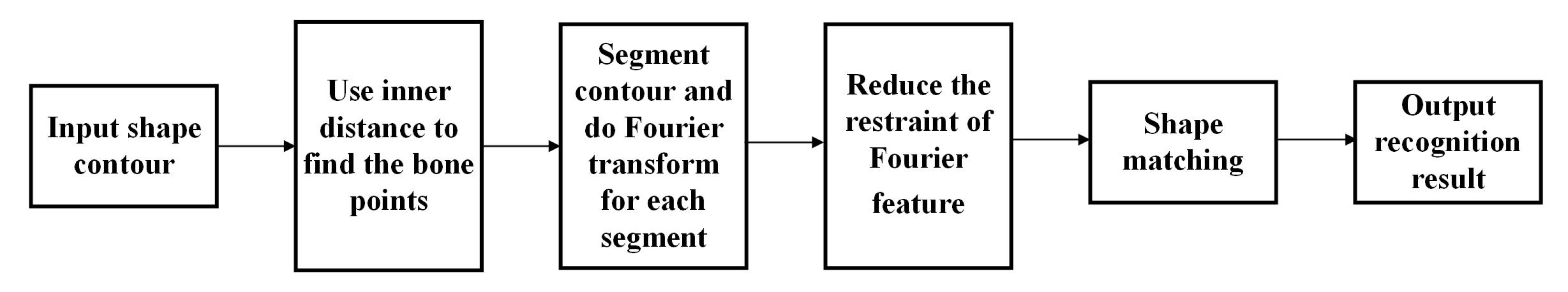
In this section, the detailed procedure of the proposed method is explained. It includes shape bone points generation strategy, shape contour segmentation strategy, Fourier feature representation of each contour segment, and reduction restraint of shape feature. Among them, the generative strategies of shape bone points include concave bone points and convex bone points. The BPS method framework is shown in Figure 4. The proposed method can be divided into six parts, from the input shape contour to the output shape recognition result, which represents the complete step of shape recognition. See Section 3 for a detailed comparison and evaluation.

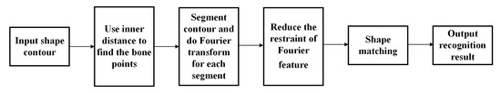
Figure 4. Framework of the proposed fast shape recognition method via the restraint reduction of BPS.

The proposed method can be divided into six parts, from the input shape contour to the output shape recognition result, which represents the complete step of shape recognition. See Section 3 for a detailed comparison and evaluation. The pseudo-code of BPS is listed in Algorithm 1.

Algorithm 1

Input: Shape contour sampling points, $\left\{P_1,P_2,P_3,\dots ,P_{N_i}\right\}$;

Output: Shape recognition similarity of reduction restraint, $di{s}_{f}r$;

1: Create some sets $P_c\leftarrow ⌀,P_v\leftarrow ⌀,P_b\leftarrow ⌀$,

2: for each $m\in \left[1,N_i\right]$, do

3: if Euclidean distance = Inner distance, and the line of two points intersects with shape contour only at three points do;

4: $P_c\leftarrow P_m$;

5: end if

6: Calculate the convex bone points according to the concave bone points, $P_v\leftarrow P_m,P_b\leftarrow \left(P_c\bigcup P_v\right)$;

7: end for

8: Segment shape contour with bone points, $P_b$;

9: N represents the number of segments, $N\in [1,b]$;

10: Fourier transform on the each of segment to form the Fourier feature of $F_{BPS}^i=\left[F_{BPS}^1,F_{BPS}^N\left(k\right),\dots ,F_{BPS}^N\left(k\right)\right]$;

11: Reduce restraint for $F_{BPS}^i\left(k\right)$ to obtain the low restraint of Fourier feature $F_{BPSr}^i=\left[F_{BPSr}^1,F_{BPSr}^2,\dots ,F_{BPSr}^{\left(N_r\right)}\right]$, $N_r$ represents the number of Fourier features of segment under reduction restraint;

12: Then, shape matching and shape recognition, get recognition accuracy.

13: Return

3.1. Shape Bone Point

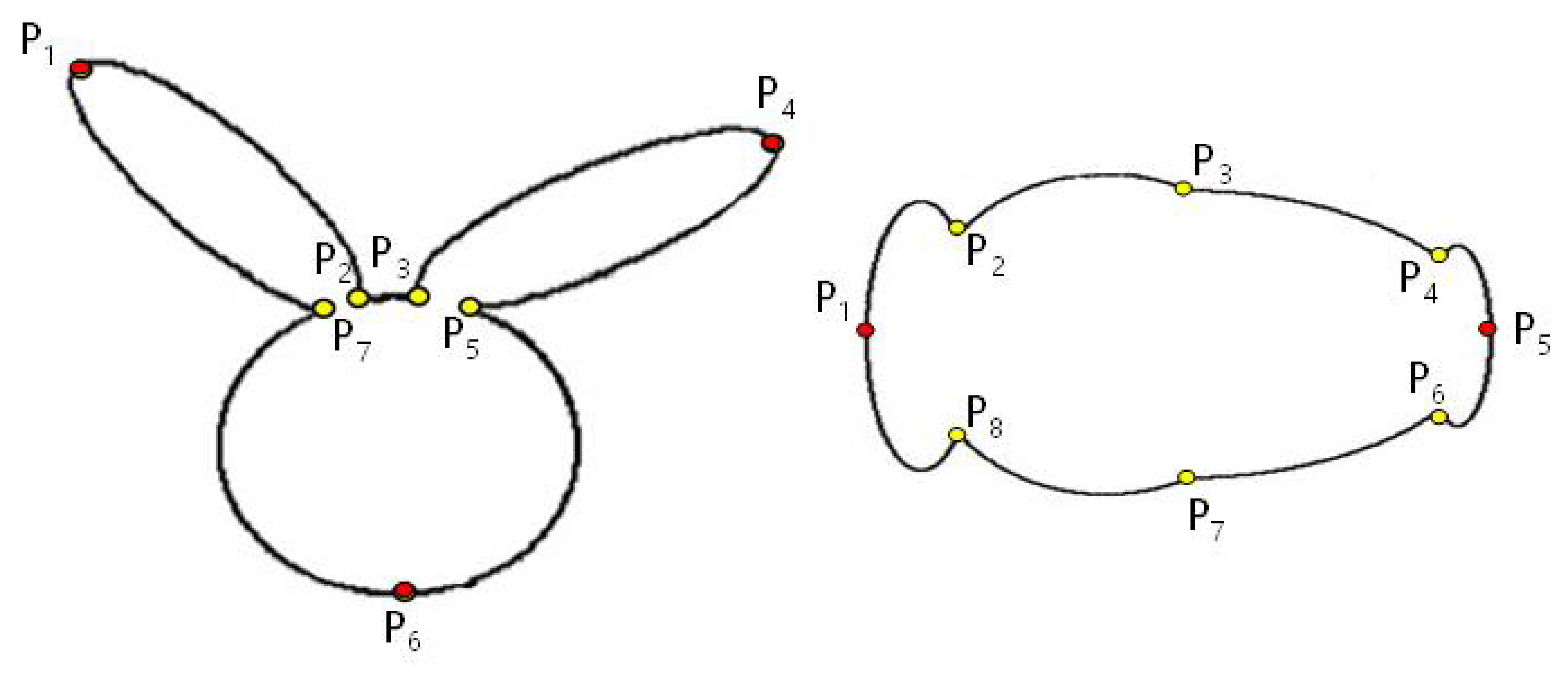
Generally speaking, bone points are the highest and lowest points in the structure of the skull (everyone pays more attention to the raised bone points, but the concave bone points are easily ignored, and are also indispensable to the skull structure). Lacking function, with the existence of bone points, the skull will have its ups and downs and a turning point; otherwise, the skull is really just a few planes. Bone points play more important roles in the structure of the skull, such as height, undulation, front and back, turning, and more importantly, the sense of space, etc. These are the focus of research on bone points. The shape bone point is expressed as the turning point of the shape contour protrusion or depression. Different shapes show different bone points. According to the shape and contour of the bone points, the unique protrusion or depression line segment can be obtained, expressed as a single peak in mathematical theory. The bone point shape itself is a shape feature, and the partial contour segmented by the bone points is also a feature of the shape, so the bone point shapes and partial contour segmented by the bone points can be used to describe the shape feature. There are also many ways to find out the shape of bone points, such as manual observation, graphics and algorithms, and mathematical solutions. This paper uses the inner distance of the shape contour points to acquire the shape bone points, including concave bone points and convex bone points. Figure 5 marks all the bone points of a few simple shapes.

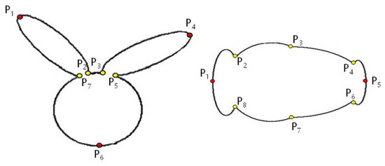
Figure 5. Two shapes. The shape contour marked shows all the bone points calculated by inner distance. Among them, yellow dot is the shape of concave bone points, and red dot is the shape of convex bone points.

3.1.1. The Generative Strategy of Concave Bone Points

In the method proposed in this paper, the concave bone points of the shape contour are first obtained. As shown in Figure 5, the yellow dots are the concave bone points of the shape contour.

Step 1: Obtain the coordinate values of the contour points of the shape and sample the contour points, in this paper the author sampled 100 contour points. After sampling is completed, each sampling point is used as the starting point to get the Euclidean distance and the inner distance between the current point and all the other contour points;

Step 2: Compare the value of the Euclidean distance and the inner distance. If the Euclidean distance between two points on the contour is less than the inner distance, it means that part of the segment between the two points is concave. At the same time, it indicates that there is at least one bone point shape between the two points;

Step 3: If the Euclidean distance from the one contour point to another point is equal to the inner distance, and the line of distance between the two points intersects at the same time with the shape contour only at three points, there is a bone point shape at the middle point;

Step 4: Repeat the operation of Step 3 until all the concave bone points of the shape contour are found.

3.1.2. The Generative Strategy of Convex Bone Points

After acquiring all concave bone points of the shape, this paper uses concave bone points to obtain shape convex bone points, and the red dots in Figure 4 are shape contour convex bone points. The generative strategy of convex bone points is as follows:

Step 1: Set the amplitude of the two adjacent concave bone points to 0, and calculate the amplitude of all contour points on the contour segment between the two bone points;

Step 2: Judge the value of the amplitude. If the maximum value is greater than a certain set threshold, it is considered that the maximum value is the convex bone point of this contour segment; otherwise, there is no convex bone point in the contour segment;

Step 3: Repeat the above steps until you find the convex bone points of all contour segments. According to the above two bone point generative strategies, this paper uses internal distance to generate all shaped bone points.

3.2. BPS of Shape

Generally speaking, the features of the part of the segment are also the features of the overall shape contour. For some shapes, the more detailed the segments of the shape contour, the more completely the features of a shape can be fully expressed. It may be because of the difference in the small parts that two shapes with extremely similar features can be distinguished. Therefore, for the partial structure of the shape segmented by the shape bone points, the more complete the bone points found, the more robust the partial shape feature obtained by segmentation. In this paper, with the method of inner distance, bone points can be found completely. In theory, all of the segments obtained in this article possess a higher representativeness of the overall shape.

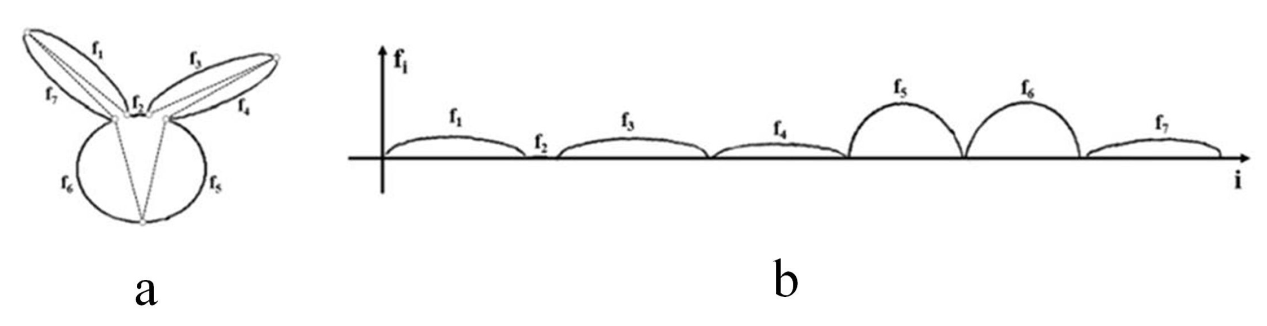
In this paper, after the shape bone points are extracted, they are connected to other bone points clockwise or counterclockwise along a certain starting bone point, and then all parts of the shape structure between the two bone points are arranged in sequence along the x-coordinate axis, where the connecting line and the x-coordinate axes coincide. At this time, there is a set of discrete point sequences on the coordinate system. Thus, the Amplitude Fourier transform can be used in the segments of the shape. The left side of Figure 6 shows the segments of the rabbit shape in Figure 5, and the right side shows the representation of the segments of the rabbit on the coordinate axis.

Figure 6. (a) shows the segments of the rabbit shape segmented by bone points; (b) shows the representation of the segments of the rabbit on the coordinate axis.

Obviously, the rabbit’s new shape contour can be clearly seen. As can be seen in the Figure 6, the shape of rabbit’s contour was divided into seven parts by the bone points, which can be defined as $f1,f2,f3,f4,f5,f6,f7$. And these parts segmented by seven shape bone points $p1,p2,p3,p4,p5,p6,p7$. For instance, for the part of $f1$, connect the shape bone points $p1$ and $p2$, and then put this part segment of shape on the x-axis of the two-dimensional coordinate axis and ensure that the connecting line of $p1$ and $p2$ coincides with the x-axis.

3.3. Fourier Transform for the All Segments of Shape

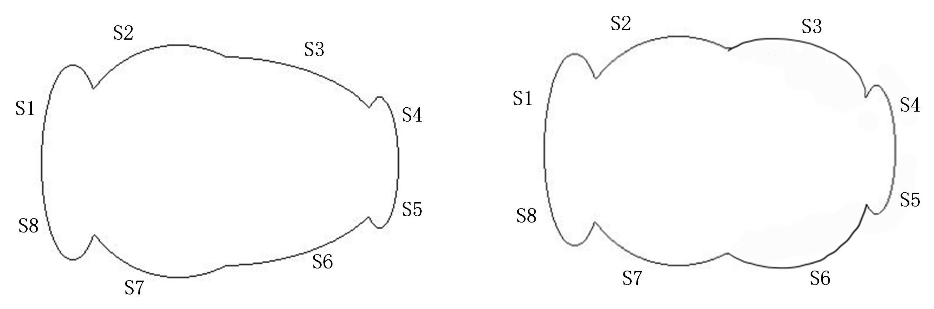
The two vase shapes are shown in Figure 7 below. After splitting the two vase shapes according to bone points, only the contour segments of S1 and S6 have significant differences, while other contour segments are relatively similar.

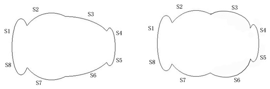
Figure 7. With the naked eye, it is easy to see that the shapes of the two vases are almost the same except that there is a big difference between the contour segments $S3$ and $S6$.

After finding the bone point shapes, segment the shape contour according to the bone points and arrange the segmented segments on the coordinate axis in order (like the right image in Figure 6). After the arrangement, a discrete sequence containing each contour segment will be formed. The discrete sequence is defined as $f_{BPS}^i,i=1,2,3,\dots N$, N defined as the number of segments, the sequence contains all contour points of the shape. For the vase shape, N is defined as 8.

In this paper, the author transforms all the segments from the spatial domain to the frequency domain, in order to form more robust frequency domain features, obtained with following Equation (4).

$$F_{BPS}\left(k\right)=1/N_P\left|\sum _{(k=0)}^{\left(N_P-1\right)}{f}_{BPS}^i{e}^{\left((-j2\pi ik)/N_P\right)}\right|,k=0,1,\dots ,N_s-1$$

(4)

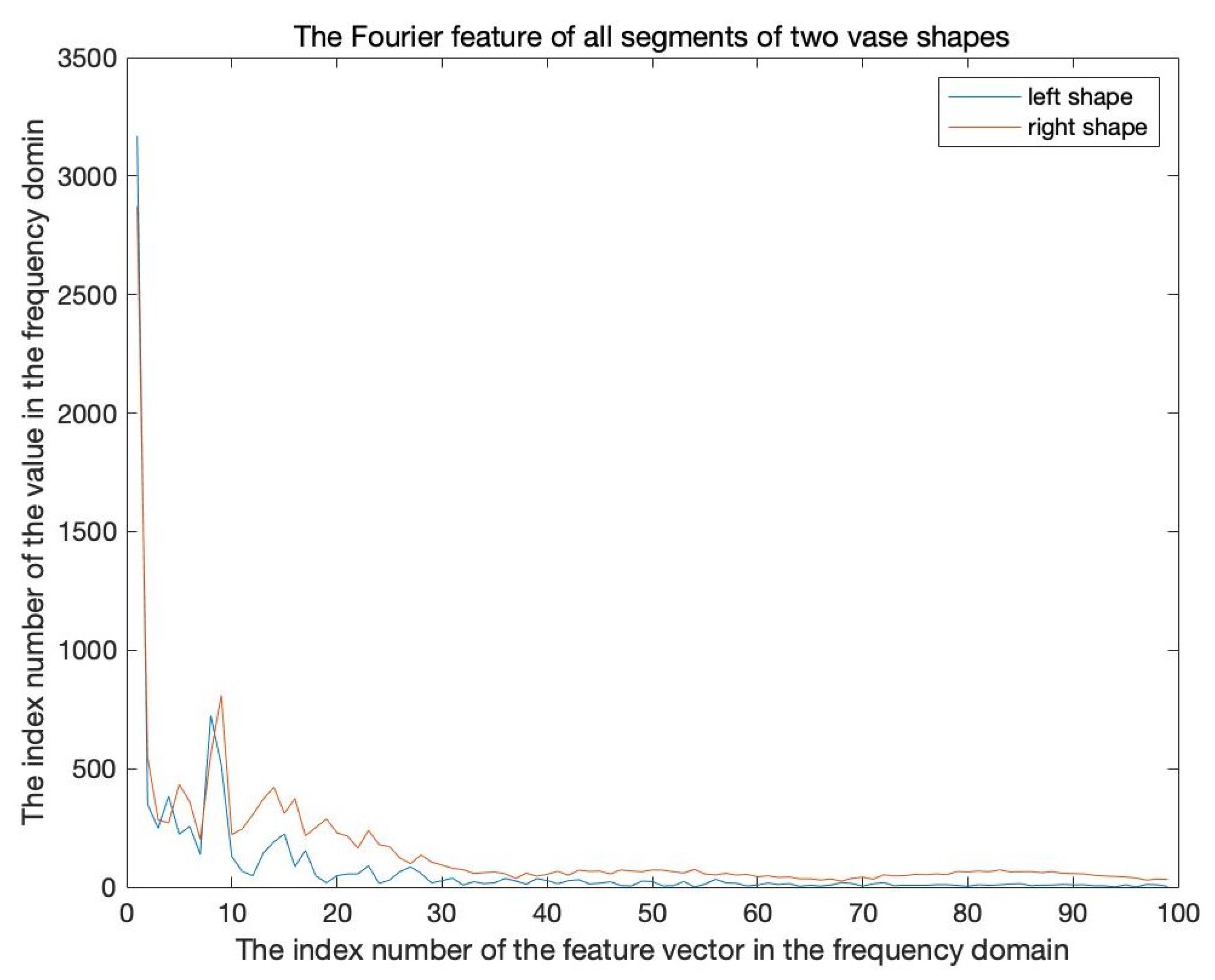
The Fourier transform results of all contour segments of this pair of shapes are shown in Figure 8 below. Obviously, the Fourier transform results of all segments of these two shapes differ greatly, so they cannot be considered as the same shape in the next stage of shape matching. This will greatly reduce the matching accuracy of the shape, thus affecting the recognition accuracy of the whole database.

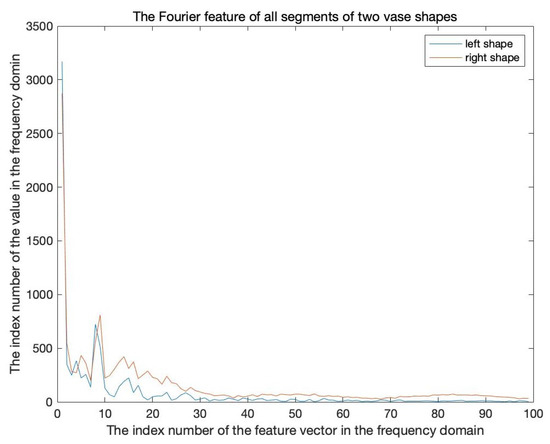
Figure 8. Fourier features of all contour segments of the two vase shapes in Figure 7. The red curve represents the Fourier feature of the left-hand shape, and the blue curve represents the Fourier character of the right-hand shape. Obviously, these two Fourier curves are very different.

3.4. Fourier Transform for the BPS Based on the Restraint Reduction

All contour segments segmented by the shaped bone points can be processed according to the method in Section 3.2. However, it is found that if different shapes of the same target are deformed in a small number of contour segments, the Fourier characteristics of the whole shape will be seriously affected, and the recognition accuracy will be greatly reduced if the whole contour segment is directly matched after the Fourier transform. However, most of the existing international general shape recognition data sets show local deformation after analysis. For example, a pair of shapes in Figure 7 are all vase shapes, but the shape features obtained by Fourier transform of all the shape bone point segments have little similarity and cannot be correctly identified and matched. It can be seen from Figure 8 that the two Fourier curves are quite different and have little similarity.

Therefore, this paper proposes a Fourier transform method of shaped bone segment based on reduction constraint. Firstly, the shape contour is segmented into corresponding contour segments using shape concave bone points, and then the Fourier transform is performed on each contour segment respectively to form a Fourier transform feature sequence $F_{BPS}^i,i=1,2,3,\dots N$, N defined as the number of segments. This paper transforms each segmented segments from the spatial domain to the frequency domain, in order to form more robust frequency domain features, obtained using Equation (5).

$$F_{BPS}^i\left(k\right)=\left[F_{BPS}^1\left(k\right),F_{B}P{S}^2\left(k\right),\dots ,F_{BPS}^N\left(k\right)\right],i=1,2,\dots ,N,k=0,1,\dots ,N-1$$

(5)

where, $F_{BPS}^i\left(k\right)$ represents the frequency domain feature of segment i, which obtains with following Equation (6)

$$F_{BPS}^i\left(k\right)=1/N_P\left|\sum _{(k=0)}^{\left(N_P-1\right)}{f}_{BPS}^i{e}^{\left((-j2\pi ik)/N_P\right)}\right|,i=1,2,\dots ,N,k=0,1,\dots ,N_P-1$$

(6)

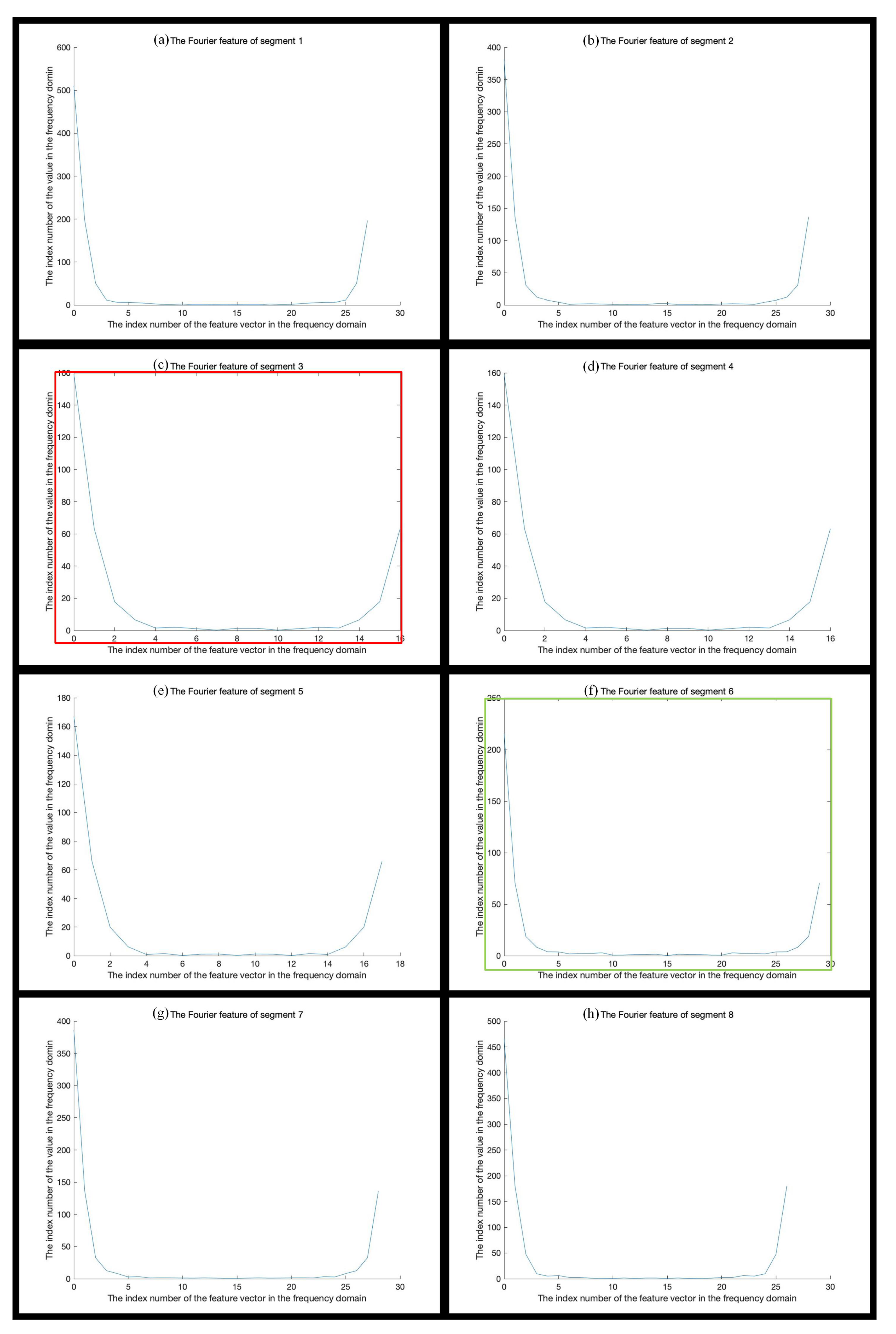
Figure 9 shows the Fourier transform curves of each contour segment of the vase shape on the left in Figure 7.

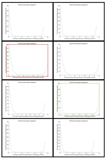
Figure 9. The Fourier transform of each contour segment of the vase shape on the left in Figure 7.

For the Fourier feature of BPSs based on the reduction restraint, this method transforms the frequency feature $F_{BPS}$ to the feature of sequence $F_{BPSr}$, which makes the constraint of global contour on Fourier feature reduced greatly. Accordingly, the local contour feature will be processed and analyzed separately and the local deformation will not affect the overall shape features. As a result, contour feature restraints will be reduced, and the matching accuracy of shapes will be greatly improved.

Figure 10 shows the Fourier transform curves of each contour segment of the vase shape on the right in Figure 7.

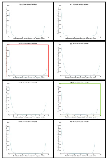
Figure 10. The Fourier transform of each contour segment of the vase shape on the right in Figure 7.

It can be seen from the Figure 9 and Figure 10 that only the Fourier feature of the segments on $S3$ and $S6$ (such as the two pairs of feature curves framed in red and green, respectively, (c) and (f)) shows the significant difference, while other segments express a mass amount of similarity. So, in the following stage of the method, the feature similarity measure can be applied to each contour segment separately. In other words, each contour segment of the current shape will be measured for similarity with all other contour segments. And a new shape feature structure based on reduction restraint will be introduced, at the same time, higher shape matching accuracy results will be obtained in this paper.

According to the above equations, the Fourier feature based on the reduction restraint can be transformed to the Equation (7).

$$F_{BPSr}^i\left(k\right)=\left[F_{BPSr}^1\left(k\right),F_{BPSr}^2\left(k\right),\dots ,F_{BPSr}^{\left(N_r\right)}\left(k\right)\right],i=1,2,\dots ,N_r,k=0,1,\dots ,N_p-1$$

(7)

where, $N_r$ represents the number of segments’ Fourier features under the reduction restraint.

3.5. Shape Dissimilarity Measurement

Shape dissimilarity measurement is a very standard method [1,2,32,33] for explaining shape matching [28,30,31,32]. The method of BPS is based on the distance in frequency domain, this paper uses the difference Equation to calculate the distance between two shapes, shown as Equation (8):

$$di{s}_f\left(s_1,s_2\right)=\sum _{(k=0)}^K\left|F_{BPS}^{\left(s_1\right)}\left(k\right)-F_{BPS}^{\left(s_2\right)}\left(k\right)\right|,0\le K\le N_P$$

(8)

where, $s1$ and $s2$ are the index numbers of two shapes and K indicates the number of coefficients of the frequency domain feature used in the matching process. In this article, K = 200 exists.

According to Section 3.4, with the reduction restrain of BPSs on Fourier feature, Equation (7) can be rewritten as Equation (9) below:

$$di{s}_f\left(s_1,s_2\right)={\sum }_{(k=0)}^K\left|\left[F_{BPS}^{s}1,1\left(k\right),F_{BPS}^{s}1,2\left(k\right),\dots ,F_{BPS}^{(s1,N1)}\left(k\right)\right]-\left[F_{BPS}^{s}2,1\left(k\right),F_{BPS}^{s}2,2\left(k\right),\dots ,F_{BPS}^{(s2,N2)}\left(k\right)\right]\right|,0\le K\le N_P$$

(9)

where, $N1$ and $N2$ represent the number of segments of shape $s1$ and $s2$, respectively. In this paper, the similarity matching is defined as the matching of Fourier features for BPS between current shape and shape to match. If one pair of Fourier features on BPSs are a matching success, the feature of current shape’s contour segment is regarded as the reduction restraint feature of the shape, expressed as $F_{BPSr}$. Otherwise, the BPS is removed. Repeating this process will obtain the feature sequence of all the bone points and segments of a shape constrained by a certain shape as the final feature of the shape. For instance, the two vase shapes in Figure 6 were matched for shape similarity. And the segments of $S3$ and $S6$ fail to match, so the feature of BPS based on reduction restraint can be written as Equation (10).

$$F_{BPSr}^{(vase,i)}\left(k\right)=\left[F_{BPS}^{(vase,1)}\left(k\right),F_{BPS}^{(vase,2)}\left(k\right),F_{BPS}^{(vase,4)}\left(k\right),F_{BPS}^{(vase,5)}\left(k\right),F_{BPS}^{(vase,7)}\left(k\right),F_{BPS}^{(vase,8)}\left(k\right)\right]$$

(10)

Therefore, according to Equation (7), the final shape matching Equation is expressed as Equation (11).

$$di{s}_{f}r\left(s_1,s_2\right)=\sum _{(k=0)}^K\left|F_{BPSr}^{\left(s_1\right)}\left(k\right)-F_{BPSr}^{\left(s_2\right)}\left(k\right)\right|,0\le K\le N_P$$

(11)

3.6. Computational Complexity

Computational complexity in shape recognition is regarded as the complexity of shape description methods [34,35,36] in feature calculation. The BPS method used in this paper is itself a mathematical calculation method with low computational complexity. Coupled with the processing of the reduction restraint in this paper, the amount of computational data is greatly reduced, so the method proposed in this paper has low computational complexity. When the input data is a certain shape contour point ($N_i$), compared with some shape description methods with the same calculation method, this paper has the lowest computational complexity. Although the BPS method also carries out the Fourier transform for all contour points, it adds the reduction restraint in the stage of shape similarity measurement, and the final total complexity is less than $O\left(N_i\right)$, which also becomes an important basis for the faster recognition speed of this method. Table 1 below lists the computational complexity of some representative shape description methods. T represents the number of iterations of the method.

Table 1. Computational complexity of some representative shape description methods.

Method	Computational Complexity
Co-transduction [22]	$O\left(T{N}_i\right)$
FD-CCD [8]	$O\left(T{N}_i\right)$
LP [32]	$O\left(T{N}_i\right)$
LCDP [22]	$O\left(T{N}_i^2\right)$
IDSC [12]	$O\left(N_i^2\right)$
SC [3]	$O\left(N_i^2\right)$
CBW [37]	$O\left(T{N}_i\right)$
BPS (ours)	O (≤$T{N}_i$)

4. Experimental Results and Analysis

In order to evaluate the performance results of the shape recognition method proposed in this paper, the shape descriptors formed by the method were respectively verified in one personal dataset collected by the author and three mainstream international general datasets (many algorithms were tested by [38,39,40,41]) for shape recognition. Including BPS 100 dataset, MPEG-7 Part B dataset, leaf dataset, and Kim 99 dataset. There are different types of 2D shapes in the three datasets, which can be used as validation datasets for shape recognition speed and accuracy performance. In the experiments in this paper, all shape recognition methods used for comparison are written in MATLAB language. Running macOS 11.6 on a personal computer with an Intel(R) Core(Inter, Santa Clara, CA, USA) (TM) i7-4850 2.30 GHz CPU and 8gb DDR3 DRAM. Since the dynamic programming procedures of IDSC [12] take a long time, for temporal comparison with other methods, it is written in C language.

4.1. Result in BPS100

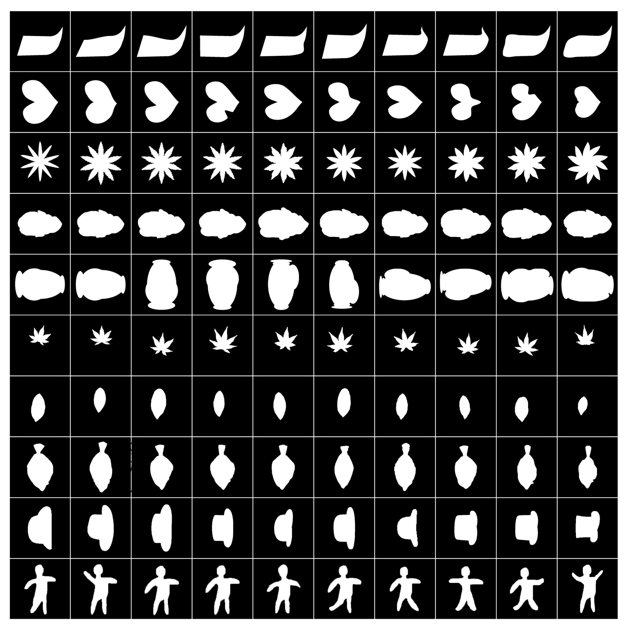
The BPS 100 dataset is a personal shape dataset built by the author in order to explain the performance of BPS based on the reduction restraint. The dataset has 100 shapes in total (10 classes, each class contains 10 shapes) collected from the general datasets of shapes on the internet. The shapes in this dataset all have a common feature (the contour of the shapes is relatively smooth and the shape bone point is relatively clear), which is very suitable for the segmentation of bone points. The shapes of 10 classes are shown in Figure 11 below. The performance and the test results of some state-of-the art descriptors are shown in Table 2, including the descriptor of BPS.

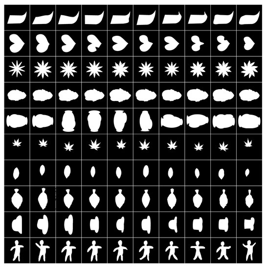
Figure 11. Some shapes collected on the internet, including 10 classes, each class has 10 shapes, which have a great amount of robustness for the BPS method.

Table 2. Recognition accuracy and matching time of BPS and some other well-known descriptors in the Swedish Plant Leaf dataset.

Descriptor	Accuracy Rate $(\%)$	Matching Time (ms)
BPS (our)	99.66	1.0
CBW [37,42]	89.78	4400.0
TCD [43]	89.90	1990.0
SC [3]	89.12	1507.0
IDSC [12]	95.13	1830.0
DIR [25]	86.60	12.3
FD-CCD [20]	75.85	3.3

4.2. Result in Mpeg-7 Part B

MPEG-7 Part B is used as a shape retrieval test dataset by a large number of researchers, and many algorithms [3,12,21,24] use this database for experiments. The dataset has a total of 1400 shape templates (70 types, each contains 20 shapes), which possess a great amount of help to the research of shape features. Figure 12 shows a part of the shape of the database. Many classical descriptors [40] are tested on this dataset. The descriptor proposed in this paper is also tested on this dataset. The performance and the test results of some well-known descriptors are shown in Table 3, including BPS.

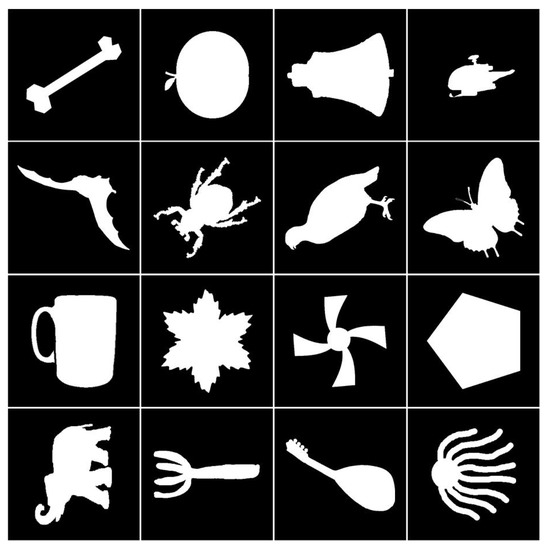
Figure 12. 16 shapes in MPEG-7 Part B dataset.

Table 3. Bull’s eye test scores and matching time of our descriptor and some other descriptors on the MPEG-7 CE1 B.

Descriptor	Bulls-Eye Score $(\%)$	Matching Time (ms)
BPS (our)	89.35	3.3
CBW [37,42]	85.20	4650
TCD  [43]	86.96	2040
SC  [3]	68.59	1060.0
IDSC [12]	85.34	1023.0
DIR [25]	77.69	12.3
FD-CCD [20]	68.94	3.6

4.3. Result in Swedish Plant Leaf

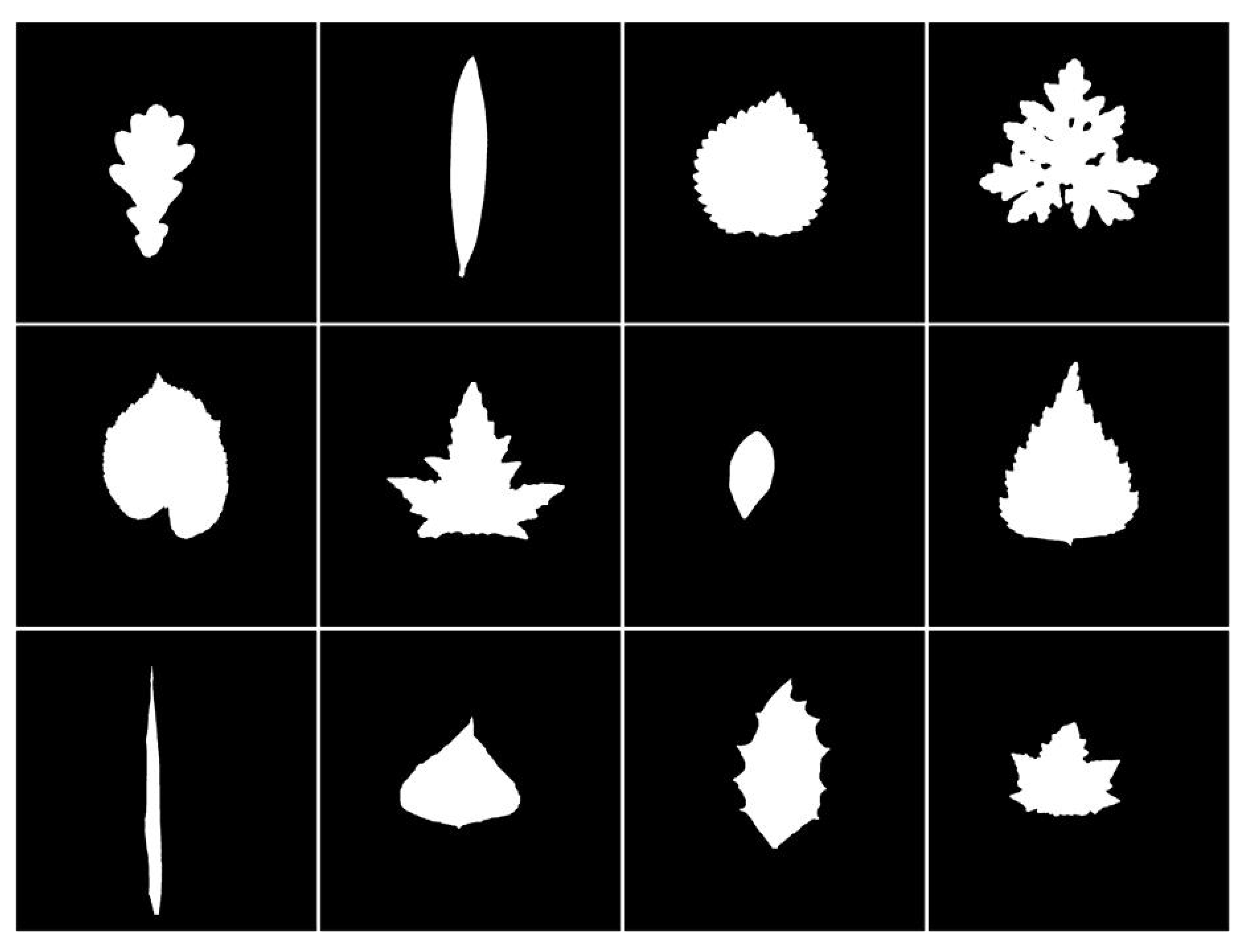
Since the BPS is a more detailed shape descriptor, it is necessary to test the result in a dataset of leaves, which have more subtle differences. The Swedish Plant Leaf is a dataset of plant leaves. It contains 1125 images divided into 15 classes, and each class contains 75 shapes. Some shapes in the dataset are shown in Figure 13. The experimental results and the test results of other famous shape descriptors are shown in Table 4, including the descriptor used here.

Figure 13. Example of shapes in Swedish Plant Leaf database. Some objects of all the 27 categories are shown.

Table 4. Accuracy rate and matching time of our descriptor and some other descriptors on the Swedish Plant Leaf dataset.

Descriptor	Accuracy Rate $\left(\%\right)$	Matching Time (ms)
BPS (our)	95.06	3.0
CBW [37,42]	93.45	4600
TCD [43]	91.06	2560
SC [3]	88.12	1054.0
IDSC [12]	94.13	1010.0
DIR [25]	67.60	11.3
FD-CCD [20]	60.85	3.8

4.4. Result in Kim99

Kim 99 is also a common shape dataset [14]. A large number of shape descriptors [41] in the article use Kim 99 as the test database. It contains 9 classes, and each class contains 11 shapes, for a total of 99 shapes. Although the dataset is small in size, it is not suitable for shape recognition methods that require a lot of learning in the early stage, but the shape contours in it are relatively comprehensive and are very suitable for validating contour-based shape description methods. Example of shapes in Kim 99 database. One object for each one of the 9 categories is shown in Figure 14. The performance and the test results of some well-known descriptors and our mehod are shown in Table 5.

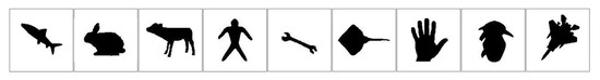
Figure 14. Example of shapes in Kim99 dataset. One object for each one of the 9 categories is shown.

Table 5. Average hit rate and matching time of the 11 most similar shapes on the Kim99.

Descriptor	Accuracy Rate $\left(\%\right)$	Matching Time (ms)
BPS (ours)	89.78	3.1
CBW [37,42]	81.25	4800
TCD  [43]	83.62	2002
DIR [25]	67.53	9.5
SC [3]	69.44	1102.0
IDSC [12]	86.00	1055.0
MDM [15]	82.72	11.1
FASD [11]	66.78	3.3
FD-CCD [20]	68.66	3.7

It can be seen from the experimental results that the contour coding reduction method proposed in this paper still has relatively high accuracy and faster matching time on the Kim 99 dataset, and the reason for its higher accuracy when compared to the Mpeg-7 dataset is that the dataset has fewer shapes, and the overall contour distribution of the shapes is more comprehensive and the overlapping of shape features is less restrained by double reduction of restraints, which is easier to identify.

4.5. To Use or Not Use Reduction Restraint

In order to verify the effectiveness of the proposed method of reduction restraint in shape recognition, a comparative experiment was conducted on the recognition accuracy between the normal restraint and the reduction restraint. The experiment is divided into two parts: the experimental result of normal restraint, the experimental result of reduction restraint in Fourier feature based on the BPS. All experiments were carried out in the above four shape datasets. The comparative experimental results are shown in Figure 15 below. It can be clearly seen from the curves that the recognition accuracy is low with the normal restraint, while the experimental results with the reduction restraint are greatly improved, even close to 100%. This shows the effectiveness of the proposed method based on reduction restraint.

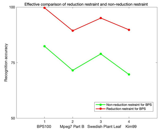
Figure 15. The recognition accuracy of reduction restraint and non-reduction restraint for BPS are tested in the four databases, the x coordinate represents four different datasets in this paper, and the y coordinate represents the recognition accuracy under different restraints.

5. Conclusions

BPS is a robust, fast, and effective shape descriptor due to its frequency domain feature and the feature reduction restraint. This method uses inner distance to obtain the key points (bone points) of the shape and segment the contour into segments. And for each segment, the Fourier transform is put into use in each. With the reduction restraint for Fourier features, the Fourier features of some severely deformed contour segments are filtered out, leaving less restrained and more outperforming Fourier feature shapes. It can be seen from the test results that the BPS approach demonstrates better description performance than other well known shape descriptors (like CBW and TCD), regardless of whether it is in the MPEG-7 Part B dataset, in the Swedish Plant Leaf dataset or in the Kim99 dataset. Further, for the BPS100 dataset, which is available on the internet and includes 100 shapes that possess clear bone points, it is worth mentioning that the recognition accuracy even approached 100%. What’s more, the speed of similarity measurements can be more than 1000 times faster than some state-of-the-art methods.

Future work will continue to enhance the theory system of reduction restraint in shape recognition, in particular with regard to structural restraint features. In order to build the engineering theory and contribute theoretical support to the practical application of shape recognition in engineering systems.

References

- Bai, X.; Yang, X.; Latecki, L.J.; Liu, W.; Tu, Z. Learning context-sensitive shape similarity by graph transduction. IEEE Trans. Pattern Anal. Mach. Intell. 2009, 32, 861–874. [Google Scholar]
- Bai, S.; Bai, X. Sparse contextual activation for efficient visual re-ranking. IEEE Trans. Image Process. 2016, 25, 1056–1069. [Google Scholar] [CrossRef] [PubMed]
- Belongie, S.; Malik, J.; Puzicha, J. Shape matching and object recognition using shape contexts. IEEE Trans. Pattern Anal. Mach. Intell. 2002, 24, 509–522. [Google Scholar] [CrossRef]
- Bonanno, E.; Ebejer, J.P. Applying machine learning to ultrafast shape recognition in ligand-based virtual screening. Front. Pharmacol. 2020, 10, 1675. [Google Scholar] [CrossRef]
- Li, Z.; Guo, B.; He, F. A multi-angle shape descriptor with the distance ratio to vertical bounding rectangles. In Proceedings of the 2021 International Conference on Content-Based Multimedia Indexing (CBMI), Lille, France, 28–30 June 2021; pp. 1–4. [Google Scholar]
- Kendall, D.G.; Barden, D.; Carne, T.K.; Le, H. Shape and Shape Theory; John Wiley & Sons: Hoboken, NJ, USA, 2009. [Google Scholar]
- Mardesic, S.; Segal, J. Shape Theory; North-Holland Publishing Company: Amsterdam, The Netherlands, 1982. [Google Scholar]
- Zhang, D.; Lu, G. Study and evaluation of different Fourier methods for image retrieval. Image Vis. Comput. 2005, 23, 33–49. [Google Scholar] [CrossRef]
- Ling, H.; Yang, X.; Latecki, L.J. Balancing Deformability and Discriminability for Shape Matching. In Proceedings of the European Conference on Computer Vision, Crete, Greece, 5–11 September 2010; Volume 6313, pp. 411–424. [Google Scholar]
- Yang, H.S.; Lee, S.U.; Lee, K.M. Recognition of 2D Object Contours Using Starting-Point-Independent Wavelet Coefficient Matching. J. Vis. Commun. Image Represent. 1998, 9, 171–181. [Google Scholar] [CrossRef]
- Zheng, Y.; Guo, B.; Chen, Z.; Li, C. A Fourier Descriptor of 2D Shapes Based on Multiscale Centroid Contour Distances Used in Object Recognition in Remote Sensing Images. Sensors 2019, 19, 486. [Google Scholar] [CrossRef] [PubMed]
- Ling, H.; Jacobs, D.W. Shape classification using the inner-distance. IEEE Trans. Pattern Anal. Mach. Intell. 2007, 29, 286–299. [Google Scholar] [CrossRef] [PubMed]
- Fotopoulou, F.; Economou, G. Multivariate angle scale descriptor of shape retrieval. In Proceedings of the Signal Processing and Applied Mathematics for Electronics and Communications Conference, Cluj-Napoca, Romania, 26–28 August 2011; pp. 26–28. [Google Scholar]
- Zhang, D.; Lu, G. Shape-based image retrieval using generic Fourier descriptor. Signal Process. Image Commun. 2002, 17, 825–848. [Google Scholar] [CrossRef]
- Hu, R.; Jia, W.; Ling, H.; Huang, D. Multiscale Distance Matrix for Fast Plant Leaf Recognition. IEEE Trans. Image Process. 2012, 21, 4667–4672. [Google Scholar]
- El-ghazal, A.; Basir, O.A.; Belkasim, S. Farthest point distance: A new shape signature for Fourier descriptors. Signal Process. Image Commun. 2009, 24, 572–586. [Google Scholar] [CrossRef]
- Ali-Dib, M.; Menou, K.; Zhu, C.; Hammond, N.; Jackson, A.P. Automated crater shape retrieval using weakly-supervised deep learning. Icarus 2020, 345, 113749. [Google Scholar] [CrossRef]
- Shen, W.; Du, C.; Jiang, Y.; Zeng, D.; Zhang, Z. Bag of Shape Features with a learned pooling function for shape recognition. Pattern Recognit. Lett. 2018, 106, 33–40. [Google Scholar] [CrossRef]
- Rakowski, A.; Wandzik, L. Hand shape recognition using very deep convolutional neural networks. In Proceedings of the 2018 International Conference on Control and Computer Vision, Singapore, 15–18 June 2018; pp. 8–12. [Google Scholar]
- Zhang, J.; Wenyin, L. A pixel-level statistical structural descriptor for shape measure and recognition. In Proceedings of the 2009 10th International Conference on Document Analysis and Recognition, Barcelona, Spain, 26–29 July 2009; pp. 386–390. [Google Scholar]
- Shu, X.; Wu, X.J. A novel contour descriptor for 2D shape matching and its application to image retrieval. Image Vis. Comput. 2011, 29, 286–294. [Google Scholar] [CrossRef]
- Bai, X.; Wang, B.; Yao, C.; Liu, W.; Tu, Z. Co-Transduction for Shape Retrieval. IEEE Trans. Image Process. 2012, 21, 2747–2757. [Google Scholar] [PubMed]
- Gu, T.; Min, R. A Swin Transformer based Framework for Shape Recognition. In Proceedings of the2022 14th International Conference on Machine Learning and Computing (ICMLC), Guangzhou, China, 18–21 February 2022; pp. 388–393. [Google Scholar]
- Chang, C.; Hwang, S.M.; Buehrer, D.J. A shape recognition scheme based on relative distances of feature points from the centroid. Pattern Recognit. 1991, 24, 1053–1063. [Google Scholar] [CrossRef]
- Kaothanthong, N.; Chun, J.; Tokuyama, T. Distance interior ratio: A new shape signature for 2D shape retrieval. Pattern Recognit. Lett. 2016, 78, 14–21. [Google Scholar] [CrossRef]
- Li, Z.; Guo, B.; Ren, X.; Liao, N.N. Vertical Interior Distance Ratio to Minimum Bounding Rectangle of a Shape. In Proceedings of the International Conference on Hybrid Intelligent Systems, Virtual Event, India, 14–16 December 2020; pp. 1–10. [Google Scholar]
- Baron Fourier, J.B.J. The Analytical Theory of Heat; The University Press: Cambridge, UK, 1878. [Google Scholar]
- Lu, Y.; Hu, C.; Zhu, X.; Zhang, H.; Yang, Q. A unified framework for semantics and feature based relevance feedback in image retrieval systems. In Proceedings of the 8th ACM international Conference on Multimedia, Los Angeles, CA, USA, 30 October– 3 November 2000; pp. 31–37. [Google Scholar]
- Cooley, J.W.; Tukey, J.W. An algorithm for the machine calculation of complex Fourier series. Math. Comput. 1965, 19, 297–301. [Google Scholar] [CrossRef]
- Devaraja, R.R.; Maskeliunas, R.; Damasevicius, R. Design and Evaluation of Anthropomorphic Robotic Hand for Object Grasping and Shape Recognition. Computers 2021, 10, 1. [Google Scholar] [CrossRef]
- Greene, E. New encoding concepts for shape recognition are needed. AIMS Neurosci. 2018, 5, 162. [Google Scholar] [CrossRef] [PubMed]
- Bicego, M.; Lovato, P. A bioinformatics approach to 2D shape classification. Comput. Vis. Image Underst. 2016, 145, 59–69. [Google Scholar] [CrossRef]
- Bai, X.; Liu, W.; Tu, Z. Integrating contour and skeleton for shape classification. In Proceedings of the ICCV Workshops of IEEE Computer Society, Kyoto, Japan, 27 September–4 October 2009; pp. 360–367. [Google Scholar]
- Zheng, A.; Cheung, G.; Florencio, D. Context tree-based image contour coding using a geometric prior. IEEE Trans. Image Process. 2016, 26, 574–589. [Google Scholar] [CrossRef] [PubMed]
- Zhang, S.; Yang, M.; Cour, T.; Yu, K.; Metaxas, D.N. Query specific rank fusion for image retrieval. IEEE Trans. Pattern Anal. Mach. Intell. 2014, 37, 803–815. [Google Scholar] [CrossRef]
- Park, W.; Jin, D.; Kim, C.S. Eigencontours: Novel contour descriptors based on low-rank approximation. In Proceedings of the IEEE/CVF Conference on Computer Vision and Pattern Recognition, New Orleans, LO, USA, 19–24 June 2022; pp. 2667–2675. [Google Scholar]
- Wang, B.; Gao, Y.; Sun, C.; Blumenstein, M.; Salle, J.L. Can Walking and Measuring Along Chord Bunches Better Describe Leaf Shapes? In Proceedings of the CVPR IEEE Computer Society Proceedings, Honolulu, HI, USA, 21–26 July 2017; pp. 2047–2056. [Google Scholar]
- Maroof, M.A.; Mahboubi, A.; Noorzad, A.; Safi, Y. A new approach to particle shape classification of granular materials. Transp. Geotech. 2020, 22, 100296. [Google Scholar] [CrossRef]
- Zhou, Y.; Zeng, F.; Qian, J.; Han, X. 3D shape classification and retrieval based on polar view. Inf. Sci. 2019, 474, 205–220. [Google Scholar] [CrossRef]
- Kumar, R.; Mali, K. Fragment of Binary Object Contour Points on the Basis of Energy Level for Shape Classification. In Proceedings of the 2021 8th International Conference on Signal Processing and Integrated Networks (SPIN), Noida, India, 26–27 August 2021; pp. 609–615. [Google Scholar]
- Wolf, B.J.; Pirih, P.; Kruusmaa, M.; van Netten, S.M. Shape Classification Using Hydrodynamic Detection via a Sparse Large-Scale 2D-Sensitive Artificial Lateral Line. IEEE Access 2020, 8, 11393–11404. [Google Scholar] [CrossRef]
- Wang, B.; Gao, Y.; Sun, C.; Blumenstein, M.; Salle, J.L. Chord Bunch Walks for Recognizing Naturally Self-Overlapped and Compound Leaves. IEEE Trans. Image Process. 2019, 28, 5963–5976. [Google Scholar] [CrossRef]
- Yang, C.; Wei, H.; Yu, Q. A novel method for 2D nonrigid partial shape matching. Neurocomputing 2018, 275, 1160–1176. [Google Scholar] [CrossRef]
Publisher’s Note: MDPI stays neutral with regard to jurisdictional claims in published maps and institutional affiliations. |
© 2022 by the authors. Licensee MDPI, Basel, Switzerland. This article is an open access article distributed under the terms and conditions of the Creative Commons Attribution (CC BY) license (https://creativecommons.org/licenses/by/4.0/).