Existence and Uniqueness of Generalized Solutions of Variational Inequalities with Fourth-Order Parabolic Operators in Finance

Abstract

In the present study, we analyze a kind of variation-inequality problem based on symmetric structure, which also incorporates fourth-order parabolic operators with a degenerate type. The penalty method is used to construct the approximate solution of the variation-inequality problem, and then the existence and uniqueness of the generalized solution are studied by a limit approximation method.

1. Introduction

Suppose $\mathsf{\Omega }\subset {\mathrm{R}}_N(N\ge 2)$ is a connected bounded region and $0<T<\infty$. We study a kind of variation-inequality problem which can be stated as follows:

$$\left\{\begin{array}{c}min\{Lu,u-u_0\}=0,(x,t)\in Q_T,\hfill \\ u(0,x)=u_0\left(x\right),x\in \mathsf{\Omega },\hfill \\ u(t,x)=0,(x,t)\in \mathsf{\partial }\mathsf{\Omega }\times (0,T),\hfill \end{array}\right.$$

(1)

with fourth-order parabolic operators, where

$$Lu=\mathsf{\partial }u+\Delta ({\rho }^{\alpha }\left(u\right){\left|\Delta u\right|}^{p-2}\Delta u),$$

$\alpha >0$ and $p>2$ are both constants. $\Delta u$ represents the second partial derivative of the space variable of u. $\rho$ is a distance function satisfies $\rho =\mathrm{dist}(x,\mathsf{\partial }\mathsf{\Omega })$. The variation-inequality problem (1) is divided into two symmetric parts based on the positional relationship between $u(x,t)$ and $u_0\left(x\right)$. When $u(x,t)>u_0\left(x\right)$ for any $(x,t)\in {\mathsf{\Omega }}_T$, $Lu=0$ in $Q_T$, whereas $Lu>0$ holds.

The variation-inequality problem has a good application in the financial field [1,2,3]. Under the following B-S model, American options and their derivatives can be transformed into a variational inequality model. In addition, the mortgage problem with a default mechanism can also be transformed into a variational inequality problem. Because the variational inequality problem has no analytical results, scholars often use numerical methods or differential equation theory to study it.

In recent years, the research on the existence, uniqueness and the properties of the solutions has attracted more and more attention to the variation-inequality problem with a second order parabolic operator. We refer to the bibliography [1,2,3,4,5,6,7] in which the American option pricing in the financial market can also establish such a variation-inequality model through a series of transformations [8,9]. Starting from the generalized solution of the penalty problem, the generalized solution of the variation-inequality problem is analyzed by the limit approximation method with the following operator

$$Lu={\mathsf{\partial }}_{t}u-u·\mathrm{div}\left(\right|\nabla u{|}^{p-2}\nabla u)-\gamma |\nabla u{|}^p.$$

The case that $Lu$ is linear parabolic operator, the existence and uniqueness results are obviously also studied [9]. Later, a two-dimensional variation-inequality system has attracted the attention of scholars [10]. Based on fixed point theorem and combined with a full mapping operator, the unique solvability theorem was analyzed. There are still a lot of literature on the theoretical research of this kind of problem, which will not be discussed here [11].

In order to study the existence, the authors of this paper mainly use comparison theorem and penalty method to construct some differential equations with approximate solutions using a recursive technique. Then, we obtain the existence of solutions to the system (1). Of course, the uniqueness of the generalized solution is also analyzed by the inequality technique.

The first innovation of this paper is to study the existence and uniqueness of solutions to variation-inequality problems under the fourth-order degenerate parabolic operators, which is coupled with a distance function. The second innovation of this paper is that compared with other references, this paper also analyzes the stability of generalized solutions.

This paper is divided into four parts. Section 1 is the introduction. In Section 2, we list the main results of this paper. Section 3 gives some estimates about penalty problems to be used to prove our main results. The proof of the main results is arranged in Section 4.

2. The Main Results of Generalized Solutions

Inspired by [1,2,3], we use the following maximal monotone operator to depict (1)

$$G\left(x\right)=\left\{\begin{array}{c}0,x>0,\hfill \\ 1,x=0.\hfill \end{array}\right.$$

(2)

This paper try to study the theoretical results of the generalized solution of problem (1). Combined with the idea of [1,2,3], we give the necessary conditions for weak solutions, and define them as follows:

Definition 1.

Function $u=(u,\xi )$ is called a generalized solution of the systems (1), if $u\in C^1(0,T;L^2\left(\mathsf{\Omega }\right))\cap L^{\infty }(0,T,L^2\left(\mathsf{\Omega }\right))$, ${\mathsf{\partial }}_{t}u\in L^2\left({\mathsf{\Omega }}_T\right)$,$\xi \in L^{\infty }(0,T;L^{\infty }\left(\mathsf{\Omega }\right))$, ${\rho }^{\alpha }{\left|\Delta u\right|}^p\in L^1\left(Q_T\right)$, $\Delta u\in L^p\left(Q_T\right)$ and satisfies

(a) 

$u(x,t)\ge u_0\left(x\right)$,

(b) 

$u(x,0)=u_0\left(x\right)$,

(c) 

$\xi \in G(u-u_0)$,

(d) 

For each $\phi \in L^p(0,T;{\mathcal{W}}_0^2\left({\overline{\mathsf{\Omega }}}_T\right))\cap L^2\left(Q_T\right)$, it has

$$\int {\int }_{{\mathsf{\Omega }}_T}({\mathsf{\partial }}_{t}u·\phi +{\rho }^{\alpha }{\left|\Delta u\right|}^{p-2}\Delta u\Delta \phi )\mathrm{d}x\mathrm{d}t={\int }_0^t{\int }_{\mathsf{\Omega }}\xi ·\phi \mathrm{d}x\mathrm{d}t,$$

(3)

where ${\mathcal{W}}_0^2\left(\mathsf{\Omega }\right)=W_0^{1,p}\left(\mathsf{\Omega }\right)\cap W_{}^{2,p}\left(\mathsf{\Omega }\right)$.

Let us show our main results as follows. For convenience, we use C to denote a positive constant.

Theorem 1.

Assume that $u_0\in L^{\infty }\left({\mathsf{\Omega }}_T\right)$ and ${\rho }^{\alpha }{\left|\Delta u_0\right|}^p\in L^1\left(\mathsf{\Omega }\right)$. Then, (1) admits a unique solution u in the sense of Definition 1.

Theorem 2.

Suppose that $(u_i,{\xi }_i)$ is a generalized of (1) with initial values $u(0,x)=u_{0,i}\left(x\right),x\in \mathsf{\Omega },i=1,2.$ Then, we have

$$|u_1-u_2|{|}_{L^2\left({\mathsf{\Omega }}_T\right)}\le \left|\right|u_{0,1}(·)-u_{0,2}(·)|{|}_{L^2\left(\mathsf{\Omega }\right)},$$

(4)

$$\left|\right|u_1-u_2|{|}_{L^2(0,T;W^{2,p}{\mathsf{\Omega }}_T)}\le C\left|\right|u_{0,1}(·)-u_{0,2}(·)|{|}_{L^2\left(\mathsf{\Omega }\right)}.$$

(5)

Hereafter, we state the following lemma, which will be used later [12,13].

Lemma 1.

Let $A\left(\tau \right)={\left|\tau \right|}^{p(x,t)-2}\tau$, $p\ge 2$, then $\forall x_1,x_2\in {\mathrm{R}}^N$,

$$\left(A\left(x_1\right)-A\left(x_2\right)\right)·(x_1-x_2)\ge {\int }_0^1|s{x}_1-(1-s)x_2{|}^{p-2}\mathrm{d}s\times {\left|x_1-x_2\right|}^2,$$

(6)

$$\left(A\left(x_1\right)-A\left(x_2\right)\right)·(x_1-x_2)\ge C\left(p\right)·{\left|x_1-x_2\right|}^p.$$

(7)

Moreover, there exists a constant C independent of M such that

$$|A\left(\xi \right)-A\left(x_2\right)|\le C\left|{\int }_0^1|s{x}_1-(1-s)x_2{|}^{p-2}\mathrm{d}s\right|·\left|x_1-x_2\right|.$$

(8)

3. A Penalty Problem

Since the operator “min” is not differentiable, we need to study an initial boundary value problem with penalty function

$$\left\{\begin{array}{c}{L}_{\epsilon }^{}{u}_{\epsilon }^{}=-{\beta }_{\epsilon }(u_{\epsilon }^{}-u_0),(x,t)\in Q_T,\hfill \\ u_{\epsilon }^{}(x,0)=u_{0\epsilon }^{}\left(x\right)=u_0+\epsilon ,x\in \mathsf{\Omega },\hfill \\ u_{\epsilon }^{}(x,t)=\epsilon ,(x,t)\in \mathsf{\partial }{Q}_T,\hfill \end{array}\right.$$

(9)

In this way, we first analyze the weak solutions of the above problems. Here, the parabolic operator is

$$L_{\epsilon }^{}{u}_{\epsilon }^{}=\frac{\mathsf{\partial }{u}_{\epsilon }^{}}{\mathsf{\partial }t}-\Delta \left({\rho }_{\epsilon }^{\alpha }{\left(\right|\Delta u_{\epsilon }^{}{|}^2+\epsilon )}^{\frac{p-2}{2}}\Delta u_{\epsilon }^{}\right).$$

Here, ${\rho }_{\epsilon }=\rho +\epsilon$, the penalty mapping ${\beta }_{\epsilon }(·)$ satisfies

$$\begin{array}{c}\epsilon \in (0,1), {\beta }_{\epsilon }(·)\in C^2\left(\mathrm{R}\right), {{\beta }^{\prime }}_{\epsilon }\left(\tau \right)\ge 0,{{\beta }^{\prime \prime }}_{\epsilon }\left(\tau \right)\le 0,\hfill \\ {\beta }_{\epsilon }\left(\tau \right)=\left\{\begin{array}{cc}0& \tau \ge \epsilon ,\\ -1& \tau =0,\end{array}\right.\underset{\epsilon \to 0+}{lim}\beta \left(\tau \right)=\left\{\begin{array}{c}0,\tau >0,\hfill \\ -1,\tau =0.\hfill \end{array}\right.\hfill \end{array}$$

(10)

An important result is that if $u>u_0$, $Lu=0$, and if $u=u_0$, one gets $Lu\ge 0$ in (1) that ${\beta }_{\epsilon }(u_{\epsilon }^{}-u_0)$ plays a similar role in (9). If $u_{\epsilon }^{}>u_0+\epsilon$,

$$L_{\epsilon }^{}{u}_{\epsilon }^{}=-{\beta }_{\epsilon }(u_{\epsilon }^{}-u_0)=0,$$

and if $u_0\le u_{\epsilon }^{}\le u_0+\epsilon$, we have

$$L_{\epsilon }^{}{u}_{\epsilon }^{}=-{\beta }_{\epsilon }(u_{\epsilon }^{}-u_0)\ge 0.$$

With a similar method as in [10], problem (9) admits a unique generalized solution satisfies

$$u_{\epsilon }\in C^1(0,T;L^2\left(\mathsf{\Omega }\right))\cap L^{\infty }(0,T,L^2\left(\mathsf{\Omega }\right)),{\mathsf{\partial }}_t{u}_{\epsilon }\in L^2\left({\mathsf{\Omega }}_T\right),$$

satisfying the following integral identities

$$\int {\int }_{{\mathsf{\Omega }}_T}({\mathsf{\partial }}_t{u}_{\epsilon }·\phi +{\rho }_{\epsilon }^{\alpha }{\left|\Delta u_{\epsilon }\right|}^{p-2}\Delta u_{\epsilon }\Delta \phi )\mathrm{d}x\mathrm{d}t=-\int {\int }_{\mathsf{\Omega }}{\beta }_{\epsilon }(u_{\epsilon }-u_0)\phi \mathrm{d}x\mathrm{d}t$$

(11)

with $\phi \in L^p(0,T;{\mathcal{W}}_0^2\left({\overline{\mathsf{\Omega }}}_T\right))\cap L^2\left(Q_T\right)$.

We first prove some estimates of penalty problem (9). For that reason, we give a comparison principle.

Lemma 2.

If $L_{\epsilon }{u}_{\epsilon }\ge L_{\epsilon }{v}_{\epsilon }$ in $Q_T$, $u_{\epsilon },v_{\epsilon }\in L^p(0,T;W^{1,p}\left(\mathsf{\Omega }\right))$ and $u_{\epsilon }(x,t)\le v_{\epsilon }(x,t)$ on $\mathsf{\partial }{Q}_T$, then $u_{\epsilon }(x,t)\le v_{\epsilon }(x,t)$ in $Q_T$.

Proof. 

Assume that $u_{\epsilon }(x,t)$ and $v_{\epsilon }(x,t)$ satisfy $L_{\epsilon }{u}_{\epsilon }\ge L_{\epsilon }{v}_{\epsilon }$ in $Q_T$, and there exists a positive number $\delta >0$, such that $w=u_{\epsilon }-v_{\epsilon }>\delta$ holds on a nonempty set

$${\mathsf{\Omega }}_{\delta }=\mathsf{\Omega }\cap \{x:w(x,t)>\delta \}.$$

Then, we multiply $L_{\epsilon }{u}_{\epsilon }\ge L_{\epsilon }{v}_{\epsilon }$ by w and integrate in $Q_{\delta }={\mathsf{\Omega }}_{\delta }\times (0,T)$ to have

$$J_1+J_2\le 0,$$

(12)

where

$$J_1={\int }_{Q_{\delta }}\frac{\mathsf{\partial }}{\mathsf{\partial }t}w·w\mathrm{d}x,J_2={\rho }_{\epsilon }^{\alpha }{\int }_{Q_{\delta }}[{\left(|\Delta u_{\epsilon }^{}{|}^2+\epsilon \right)}^{\frac{p-2}{2}}\Delta u_{\epsilon }^{}-{\left(|\Delta v_{\epsilon }^{}{|}^2+\epsilon \right)}^{\frac{p-2}{2}}\Delta v_{\epsilon }^{}]\Delta w\mathrm{d}x.$$

By virtue of the first inequality of Lemma 2, we have

$$J_2\ge 2^{-p}\int {\int }_{Q_{\tau ,\epsilon }}|w{|}^p\mathrm{d}x\mathrm{d}t\ge 0.$$

(13)

We drop the nonnegative terms (13) in (12) to arrive at

$$\frac{1}{2}\frac{\mathrm{d}}{\mathrm{d}t}{\int }_{Q_{\delta }}{w}^2\mathrm{d}x\le 0.$$

(14)

It follows by $u(x,t)\le v(x,t)$ on $\mathsf{\partial }{Q}_T$ that

$${\int }_{{\mathsf{\Omega }}_{\delta }}{w}^2\mathrm{d}x\le {\int }_{Q_{\delta }}|u_{\epsilon }(x,0)-v_{\epsilon }(x,0){|}^2\mathrm{d}x=0.$$

(15)

This implies $|{\mathsf{\Omega }}_{\delta }|=0$, and Lemma 2 is proved by a contradiction. □

Lemma 3.

For any $(x,t)\in {\mathsf{\Omega }}_T$, the following inequalities hold

$$u_{0\epsilon }\le u_{\epsilon }\le {\left|u_0\right|}_{\infty }+\epsilon ,$$

(16)

$$u_{{\epsilon }_1}\le u_{{\epsilon }_2}\mathrm{for}{\epsilon }_1\le {\epsilon }_2.$$

(17)

Proof. 

Arguing by contradiction, we first prove $u_{\epsilon }\ge u_{0\epsilon }$. Assume that $u_{\epsilon }\le u_{0\epsilon }$ in $Q_T^0\subset Q_T$. Noting that $u_{\epsilon }\ge u_{0\epsilon }$ on $\mathsf{\partial }{Q}_T$, one can easily gets that $u_{\epsilon }=u_{0\epsilon }$ on $\mathsf{\partial }{\mathrm{Q}}_T^0$. Moreover, we let $t=0$ in (9) to arrive at

$$L{u}_{0,\epsilon }=-{\beta }_{\epsilon }(u_{0,\epsilon }-u_0)=0,$$

(18)

$$L_{\epsilon }{u}_{\epsilon }=-{\beta }_{\epsilon }(u_{\epsilon }-u_{0,\epsilon })\le 0.$$

(19)

Applying Lemma 2 easily obtains

$$u_{\epsilon }(x,t)\ge u_{0,\epsilon }\left(x\right)\mathrm{for}\mathrm{any}(x,t)\in Q_T^0.$$

(20)

Therefore, we obtain a contradiction.

Second, we focus on $u_{\epsilon }(t,x)\le |u_0{|}_{\infty }+\epsilon$. From the definition of ${\beta }_{\epsilon }(·)$, we have for any $(x,t)\in Q_T$,

$$L\left(\right|u_0{|}_{\infty }+\epsilon )=0,L_{\epsilon }{u}_{\epsilon }=-{\beta }_{\epsilon }(u_{\epsilon }-u_0)\ge 0.$$

(21)

Using Lemma 2 to (21) and the fact that $u_{\epsilon }\le |u_0{|}_{\infty }+\epsilon \mathrm{on}\mathsf{\partial }\mathsf{\Omega }\times (0,T)$, we know that

$$u_{\epsilon }(t,x)\le |u_0{|}_{\infty }+\epsilon \mathrm{in}{Q}_T.$$

(22)

Combining (21) and (22) and using Lemma 2 again, the second part of (16) holds.

Third, we analyze (17) by contradiction. Assume that $u_{{\epsilon }_1}>u_{{\epsilon }_2}$ in $Q_T^1\subset Q_T$. Recall that ${\epsilon }_1\le {\epsilon }_2$. Applying the definition of ${\beta }_{\epsilon }(·)$ and (9), one gets $u_{{\epsilon }_1}\le u_{{\epsilon }_2}$ on $\mathsf{\partial }{Q}_T$. Then, we may conclude that $u_{{\epsilon }_1}=u_{{\epsilon }_2}$ on $\mathsf{\partial }{\mathrm{Q}}_T^1$. It follows by Lemma 2 that

$$L{u}_{{\epsilon }_1}=-{\beta }_{{\epsilon }_1}(u_{{\epsilon }_1}-u_0),L{u}_{{\epsilon }_2}=-{\beta }_{{\epsilon }_2}(u_{{\epsilon }_2}-u_0),$$

Subtracting two equations, we have

$$L{u}_{{\epsilon }_1}-L{u}_{{\epsilon }_2}={\beta }_{{\epsilon }_2}(u_{{\epsilon }_2}-u_0)-{\beta }_{{\epsilon }_1}(u_{{\epsilon }_1}-u_0)\ge {\beta }_{{\epsilon }_2}(u_{{\epsilon }_1}-u_0)-{\beta }_{{\epsilon }_1}(u_{{\epsilon }_1}-u_0)>0.$$

Recall that $u_{{\epsilon }_1}>u_{{\epsilon }_2}$ in $Q_T^1$. Applying Lemma 2 easily obtains

$$u_{{\epsilon }_1}\le u_{{\epsilon }_2}\mathrm{in}{\mathrm{Q}}_T^1$$

This leads to a contradiction. □

Lemma 4.

For any $(x,t)\in {\mathsf{\Omega }}_T$, the solution of problem (9) satisfies the estimate

$$\int {\int }_{Q_T}{\rho }_{\epsilon }^{\alpha }|\Delta u_{\epsilon }{|}^p\mathrm{d}x\mathrm{d}t\le C,\int {\int }_{Q_T}{\rho }_{\epsilon }^{\alpha }{\left(\right|\Delta u_{\epsilon }{|}^2+\epsilon )}^{\frac{p-2}{2}}|\Delta u_{\epsilon }^{}{|}^2\mathrm{d}x\mathrm{d}t\le C.$$

(23)

Here, positive constant C is independent of ε.

Proof. 

We first prove the right inequality of (23). Choosing $\phi =u_{\epsilon }^{}$ as a test function in (11), it follows that

$$\int {\int }_{Q_T}{\mathsf{\partial }}_t{u}_{\epsilon }^{}·u_{\epsilon }^{}+{\rho }_{\epsilon }^{\alpha }{\left(\right|\Delta u_{\epsilon }{|}^2+\epsilon )}^{\frac{p-2}{2}}\Delta {u_{\epsilon }}^2\mathrm{d}x\mathrm{d}t=-\int {\int }_{Q_T}{\beta }_{\epsilon }(u_{\epsilon }^{}-u_0)u_{\epsilon }^{}\mathrm{d}x\mathrm{d}t.$$

(24)

Using Differential transformation technique gives

$$\int {\int }_{Q_T}{\mathsf{\partial }}_t{u}_{\epsilon }^{}·u_{\epsilon }^{}\mathrm{d}x\mathrm{d}t=\frac{1}{2}\int {\int }_{Q_T}{\mathsf{\partial }}_t{\left(u_{\epsilon }\right)}^2\mathrm{d}x\mathrm{d}t=\frac{1}{2}{\int }_{Q_T}{u}_{\epsilon }^{}(·,T)-u_{\epsilon }^{}(·,0)\mathrm{d}x.$$

(25)

Then, we substitute (25) into (24) to arrive at

$$\begin{array}{c}\int {\int }_{Q_T}{\rho }_{\epsilon }^{\alpha }{\left(\right|\Delta u_{\epsilon }{|}^2+\epsilon )}^{\frac{p-2}{2}}|\Delta u_{\epsilon }^{}{|}^2\mathrm{d}x\mathrm{d}t\hfill \\ =-\int {\int }_{Q_T}{\beta }_{\epsilon }(u_{\epsilon }^{}-u_0)u_{\epsilon }^{}\mathrm{d}x\mathrm{d}t-\frac{1}{2}{\int }_{Q_T}{u}_{\epsilon }^{}(·,T)-u_{\epsilon }^{}(·,0)\mathrm{d}x.\hfill \end{array}$$

(26)

Applying ${\beta }_{\epsilon }\left(0\right)=-1$ in (10) obtains

$$\int {\int }_{Q_T}-{\beta }_{\epsilon }(u_{\epsilon }^{}-u_0)·u_{\epsilon }^{}\mathrm{d}x\mathrm{d}t\le \epsilon \left|\mathsf{\Omega }\right|T\le \left|\mathsf{\Omega }\right|T.$$

(27)

Hence, the left inequality of (23) is proved by combining (25), (26) and (27). Since $\mathsf{\Omega }$ is a bounded domain, the left inequality of (23) is an immediate consequence of the right one. □

Lemma 5.

Assume $u_{\epsilon }^{}$ is the solution of problem (9), such that

$${∥{\mathsf{\partial }}_t{u}_{\epsilon }^{}∥}_{L^2\left(Q_T\right)}^{}\le C(p,T,|\mathsf{\Omega }\left|\right).$$

(28)

Proof. 

We first choose $\phi ={\mathsf{\partial }}_t{u}_{\epsilon }^{}$ as a test function in (11) to find that

$$\begin{array}{c}\int {\int }_{Q_T}{\left({\mathsf{\partial }}_t{u}_{\epsilon }^{}\right)}^2\mathrm{d}x\mathrm{d}t=-\int {\int }_{Q_T}{\rho }_{\epsilon }^{\alpha }{\left(\right|\Delta u_{\epsilon }{|}^2+\epsilon )}^{\frac{p-2}{2}}\Delta u_{\epsilon }^{}\Delta {\mathsf{\partial }}_t{u}_{\epsilon }^{}\mathrm{d}x\mathrm{d}t-\int {\int }_{Q_T}{\beta }_{\epsilon }(u_{\epsilon }^{}-u_0)·{\mathsf{\partial }}_t{u}_{\epsilon }^{}\mathrm{d}x\mathrm{d}t\hfill \\ =-A_1+A_2,\hfill \end{array}$$

(29)

where

$$A_1=\int {\int }_{Q_T}{\rho }_{\epsilon }^{\alpha }{\left(\right|\Delta u_{\epsilon }{|}^2+\epsilon )}^{\frac{p-2}{2}}\Delta u_{\epsilon }^{}\Delta {\mathsf{\partial }}_t{u}_{\epsilon }^{}\mathrm{d}x\mathrm{d}t,A_2=-\int {\int }_{Q_T}{\beta }_{\epsilon }(u_{\epsilon }^{}-u_0)·{\mathsf{\partial }}_t{u}_{\epsilon }^{}\mathrm{d}x\mathrm{d}t.$$

Now, we pay attention to $A_1$. Using some differential transforms obtains

$$A_1=-\frac{1}{2}\int {\int }_{Q_T}{\rho }_{\epsilon }^{\alpha }{\left(|\Delta u_{\epsilon }^{}{|}^2+\epsilon \right)}^{\frac{p-2}{2}}{\mathsf{\partial }}_t\left(|\Delta u_{\epsilon }^{}{|}^2+\epsilon \right)\mathrm{d}x\mathrm{d}t=-\frac{1}{p}\int {\int }_{Q_T}{\mathsf{\partial }}_t{\left(|\Delta u_{\epsilon }^{}{|}^2+\epsilon \right)}^{\frac{p}{2}}\mathrm{d}x\mathrm{d}t.$$

Since $u_{0\epsilon }^{}\left(x\right)=u_0+\epsilon$, then

$$A_1\le -\frac{1}{p}\int {\int }_{Q_T}{\mathsf{\partial }}_t\left(\right|\Delta u_{\epsilon }^{}{|}^p)\mathrm{d}x\mathrm{d}t\le {\int }_{\mathsf{\Omega }}|\Delta u_0^{}(·,0){|}^p\mathrm{d}x.$$

(30)

Next, we focus on $A_2$. Applying Hölder inequalities again, we have that

$$A_2\le \frac{1}{2}\int {\int }_{Q_T}{\left[{\beta }_{\epsilon }(u_{\epsilon }^{}-u_0)\right]}^2\mathrm{d}x\mathrm{d}t+\frac{1}{2}\int {\int }_{Q_T}{\left({\mathsf{\partial }}_t{u}_{\epsilon }^{}\right)}^2\mathrm{d}x\mathrm{d}t.$$

(31)

Using ${\beta }_{\epsilon }\left(0\right)=-1$ in (10), we arrive at

$$\frac{1}{2}\int {\int }_{Q_T}{\left[{\beta }_{\epsilon }(u_{\epsilon }^{}-u_0)\right]}^2\mathrm{d}x\mathrm{d}t\le T\left|\mathsf{\Omega }\right|\le C.$$

(32)

Hence, Lemma 5 is proved by submitting (30), (31) and (32) into (29). □

4. Proof of Theorem 1

In this section, we give the proof of theorem 1. By (16), (23) and (28), we know that there are functions

$$u\in C^1(0,T;L^2\left(\mathsf{\Omega }\right))\cap L^{\infty }(0,T,L^2\left(\mathsf{\Omega }\right))\mathrm{as}\epsilon \to 0,$$

such that for some subsequence of $u_{\epsilon }$, still denoted by $u_{\epsilon }$,

$$u_{\epsilon }^{}\to u\mathrm{a}.\mathrm{e}.\mathrm{in}{Q}_T,$$

(33)

$${\rho }_{\epsilon }^{\alpha }|\Delta u_{\epsilon }{|}^p\stackrel{\mathrm{weak}}{\to }{\rho }^{\alpha }|\Delta u{|}^p\mathrm{in}{L}^1\left(Q_T\right),$$

(34)

$${\rho }_{\epsilon }^{\alpha }{\left|\Delta u_{\epsilon }^{}\right|}^{p-2}\Delta u_{\epsilon }^{}\stackrel{\mathrm{weak}}{\to }w\mathrm{in}{L}^{\frac{p}{p-1}}\left(Q_T\right),\mathrm{for}\mathrm{some}w,$$

(35)

$${\mathsf{\partial }}_t{u}_{\epsilon }^{}\stackrel{\mathrm{weak}}{\to }{\mathsf{\partial }}_{t}u\mathrm{in}{L}^2\left({\mathsf{\Omega }}_T\right),$$

(36)

where $\stackrel{\mathrm{weak}}{\to }$ stands for weak convergence.

Lemma 6.

For any $(x,t)\in {\mathsf{\Omega }}_T$, it has $w={\rho }^{\alpha }|\Delta u{|}^{p-2}\Delta u$.

Proof. 

Let $\phi \in C_0^1\left(Q_T\right)$ be a test-function in (11). Using $(u_{\epsilon }-u)\phi$ instead of $\phi$, we know that for any $(x,t)\in {\mathsf{\Omega }}_T$,

$$\begin{array}{c}\int {\int }_{{\mathsf{\Omega }}_T}({\mathsf{\partial }}_t{u}_{\epsilon }·\phi ·(u_{\epsilon }-u)\mathrm{d}x\mathrm{d}t+\int {\int }_{{\mathsf{\Omega }}_T}{\rho }_{\epsilon }^{\alpha }{\left|\Delta u_{\epsilon }\right|}^{p-2}\Delta u_{\epsilon }\Delta \phi ·(u_{\epsilon }-u)\mathrm{d}x\mathrm{d}t\hfill \\ +\int {\int }_{{\mathsf{\Omega }}_T}\phi ·{\rho }_{\epsilon }^{\alpha }{\left|\Delta u_{\epsilon }\right|}^{p-2}\Delta u_{\epsilon }·(\Delta u_{\epsilon }-\Delta u)\mathrm{d}x\mathrm{d}t\hfill \\ =-\int {\int }_{\mathsf{\Omega }}{\beta }_{\epsilon }(u_{\epsilon }-u_0)\phi ·(u_{\epsilon }-u)\mathrm{d}x\mathrm{d}t.\hfill \end{array}$$

(37)

By (33), it is easy to know that, as $\epsilon \to 0$,

$$\underset{\epsilon \to 0}{lim}\int {\int }_{{\mathsf{\Omega }}_T}\phi ·{\rho }_{\epsilon }^{\alpha }{\left|\Delta u_{\epsilon }\right|}^{p-2}\Delta u_{\epsilon }·(\Delta u_{\epsilon }-\Delta u)\mathrm{d}x\mathrm{d}t=0.$$

(38)

Moreover, Lemma 4 and (34) give ${\rho }_{\epsilon }^{\alpha }{\left|\Delta u\right|}^p\in L^1\left(Q_T\right)$, such that

$$\underset{\epsilon \to 0}{lim}\int {\int }_{{\mathsf{\Omega }}_T}\phi ·{\rho }_{\epsilon }^{\alpha }{\left|\Delta u\right|}^{p-2}\Delta u·(\Delta u_{\epsilon }-\Delta u)\mathrm{d}x\mathrm{d}t=0.$$

(39)

Applying Lemma 1, we find

$$\begin{array}{c}\left({\left|\Delta u_{\epsilon }\right|}^{p-2}\Delta u_{\epsilon }-{\left|\Delta u\right|}^{p-2}\Delta u\right)·(\Delta u_{\epsilon }-\Delta u)\hfill \\ \ge {\int }_0^1|s\Delta u_{\epsilon }+(1-s)\Delta u{|}^{p-2}\mathrm{d}s·{\left|\Delta u_{\epsilon }-\Delta u\right|}^2.\hfill \end{array}$$

(40)

Combining (38), (39) and (40), we arrive at

$$\underset{\epsilon \to 0}{lim}\int {\int }_{{\mathsf{\Omega }}_T}\phi ·{\int }_0^1|s\Delta u_{\epsilon }+(1-s)\Delta u{|}^{p-2}\mathrm{d}s·{\left|\Delta u_{\epsilon }-\Delta u\right|}^2\mathrm{d}x\mathrm{d}t=0.$$

(41)

Recall that ${\rho }_{\epsilon }^{\alpha }{\left|\Delta u\right|}^p\in L^1\left(Q_T\right)$ and ${\rho }_{\epsilon }^{\alpha }{\left|\Delta u_{\epsilon }\right|}^p\in L^1\left(Q_T\right)$. Then,

$$\begin{array}{c}\int {\int }_{{\mathsf{\Omega }}_T}{\int }_0^1|s\Delta u_{\epsilon }+(1-s)\Delta u{|}^{p-2}\mathrm{d}s\mathrm{d}x\mathrm{d}t\hfill \\ \le \int {\int }_{{\mathsf{\Omega }}_T}|\Delta u_{\epsilon }{|}^{p-2}\mathrm{d}x\mathrm{d}t+\int {\int }_{{\mathsf{\Omega }}_T}|\Delta u{|}^{p-2}\mathrm{d}x\mathrm{d}t\le C.\hfill \end{array}$$

(42)

Applying the second part of Lemma 1, one finds

$$\left||\Delta u_{\epsilon }^{}{|}^{p-2}\Delta u_{\epsilon }^{}-|\Delta u{|}^{p-2}\Delta u\right|\le C|\Delta u_{\epsilon }-\Delta u|·\left|{\int }_0^1|s\Delta u_{\epsilon }+(1-s)\Delta u{|}^{p-2}\mathrm{d}s\right|.$$

(43)

Hence we combine (41), (42) and (43) and use Hölder inequality to arrive at

$$\begin{array}{c}\left|\int {\int }_{{\mathsf{\Omega }}_T}\phi \left(|\Delta u_{\epsilon }^{}{|}^{p-2}\Delta u_{\epsilon }^{}-|\Delta u{|}^{p-2}\Delta u\right)\mathrm{d}x\mathrm{d}t\right|\hfill \\ \le {\left(\int {\int }_{{\mathsf{\Omega }}_T}\phi ·{\int }_0^1|s\Delta u_{\epsilon }+(1-s)\Delta u{|}^{p-2}\mathrm{d}s·{\left|\Delta u_{\epsilon }-\Delta u\right|}^2\mathrm{d}x\mathrm{d}t\right)}^{\frac{1}{2}}\hfill \\ \times {\left(\int {\int }_{{\mathsf{\Omega }}_T}\phi ·{\int }_0^1|s\Delta u_{\epsilon }+(1-s)\Delta u{|}^{p-2}\mathrm{d}s\mathrm{d}x\mathrm{d}t\right)}^{\frac{1}{2}}\to 0,\epsilon \to 0.\hfill \end{array}$$

That is,

$$\int {\int }_{{\mathsf{\Omega }}_T}\phi \left(|\Delta u_{\epsilon }^{}{|}^{p-2}\Delta u_{\epsilon }-|\Delta u{|}^{p-2}\Delta u\right)\mathrm{d}x\mathrm{d}t\to 0,\epsilon \to 0.$$

Hence Lemma 6 is proved. □

From Lemma 6, we may conclude that subsequence $\left\{\right|\Delta u_{\epsilon }{|}^{p-2}\Delta u_{\epsilon },0\le \epsilon \le 1\}$ converges to $\Delta w$ weakly, such that

$$|\Delta u_{\epsilon }^{}{|}^{p-2}\Delta u_{\epsilon }^{}\stackrel{w}{\to }|\Delta u{|}^{p-2}\Delta u\mathrm{in}{L}^{\frac{p}{p-1}}\left(Q_T\right)\mathrm{as}\epsilon \to \infty .$$

(44)

Lemma 7.

For any $(x,t)\in {\mathsf{\Omega }}_T$, then

$${\beta }_{\epsilon }(u_{\epsilon }-u_0)\to \xi \in G(u-u_0)\mathrm{as}\epsilon \to 0.$$

(45)

Proof. 

Using (16), (33) and the definition of ${\beta }_{\epsilon }$, we have

$${\beta }_{\epsilon }(u_{\epsilon }-u_0)\to \xi \mathrm{as}\epsilon \to 0.$$

To prove (45), we need to prove that $\xi (x,t)=0$ if $u(x,t)>u_0\left(x\right)$. Indeed, if $u(x,t)>u_0\left(x\right)$, there exist a positive constant $\lambda$ and a $\delta$-neighborhood $B_{\delta }(x_0,t_0)$ such that

$$u_{\epsilon }(x,t)\ge u_0\left(x\right)+\lambda ,\forall (x,t)\in B_{\delta }(x_0,t_0).$$

Then, for any $(x,t)\in B_{\delta }(x_0,t_0)$,

$$0\ge {\beta }_{\epsilon }(u_{\epsilon }-u_0)\ge {\beta }_{\epsilon }\left(\lambda \right)=0.$$

As $\epsilon \to 0$, one obtains

$$\xi (x,t)=0, \forall (x,t)\in B_{\delta }(x_0,t_0).$$

Hence, (45) follows. □

We know in (9) that if $u_{\epsilon }^{}>u_0+\epsilon$,

$$L_{\epsilon }^{}{u}_{\epsilon }^{}=-{\beta }_{\epsilon }(u_{\epsilon }^{}-u_0)=0,$$

and if $u_0\le u_{\epsilon }^{}\le u_0+\epsilon$, we have

$$L_{\epsilon }^{}{u}_{\epsilon }^{}=-{\beta }_{\epsilon }(u_{\epsilon }^{}-u_0)\ge 0.$$

It is worth readers noting that $\xi$ plays a similar role in Definition 1. When $u>u_0$, $\xi (x,t)=0$, and when $u_{\epsilon }^{}=u_0$, then we get $\xi (x,t)=0$. This corresponds to (1).

Proof. 

Applying (16), (17), and Lemma 7, we may conclude that

$$u(x,t)\le u_0\left(x\right),\mathrm{in}{\mathsf{\Omega }}_T,u(x,0)=u_0\left(x\right),\mathrm{in}\mathsf{\Omega },\xi \in G(u-u_0),$$

thus (a), (b), and (c) of Definition 1.1 hold. The other part of the existence proof can follow the similar way in [8]. We omit the details here. □

Proof. 

Let $(u,\xi )$ and $(v,\zeta )$ be two solutions of (1). Subtracting the two equations of (3) for $(u,\xi )$ and $(v,\zeta )$, and letting $\phi =u-v$, we find

$$\frac{1}{2}{\int }_{\mathsf{\Omega }}{\phi }^2\mathrm{d}x+{\int }_0^{\mathrm{t}}{\int }_{\mathsf{\Omega }}{\rho }^{\alpha }\left(\right|\nabla u{|}^{p-2}\nabla u-|\nabla v{|}^{p-2}\nabla v)·\nabla \phi \mathrm{d}x\mathrm{d}t={\int }_0^{\mathrm{t}}{\int }_{\mathsf{\Omega }}(\xi -\zeta )·\phi \mathrm{d}x\mathrm{d}t,$$

(46)

Now, we prove

$${\int }_0^{\mathrm{t}}{\int }_{\mathsf{\Omega }}(\xi -\zeta )·\phi \mathrm{d}x\mathrm{d}t\le 0.$$

(47)

If $u(x,t)>v(x,t)$, then $u(x,t)>u_0\left(x\right)$. Here, we used lLemma 1. From (2) and (45), it is easy to see that $\xi =0\le \zeta$. This leads to

$$(\xi -\zeta )·\phi =(\xi -\zeta )·(u-v)\le 0.$$

(48)

On the contrary, if $u(x,t)<v(x,t)$, $\xi \ge 0=\zeta$ for any $(x,t)\in {\mathsf{\Omega }}_T$, thus (48) still holds.

Next, we focus on $\left(\right|\nabla u{|}^{p-2}\nabla u-|\nabla v{|}^{p-2}\nabla v)·\nabla \phi$. Using (7), we find

$${\int }_0^{\mathrm{t}}{\int }_{\mathsf{\Omega }}{\rho }^{\alpha }\left(\right|\nabla u{|}^{p-2}\nabla u-|\nabla v{|}^{p-2}\nabla v)·\nabla \phi \mathrm{d}x\mathrm{d}t\ge C\left(p\right){\int }_0^{\mathrm{t}}{\int }_{\mathsf{\Omega }}{\rho }^{\alpha }|\nabla u-\nabla v{|}^p\mathrm{d}x\mathrm{d}t\ge 0.$$

(49)

Then, we drop the non-negative term (49) of (46) to arrive at

$$\frac{1}{2}{\int }_{\mathsf{\Omega }}{\phi }^2\mathrm{d}x={\int }_0^{\mathrm{t}}{\int }_{\mathsf{\Omega }}(\xi -\zeta )·\phi \mathrm{d}x\mathrm{d}t\le 0.$$

□

Hence, the prove of uniqueness is complete.

5. Proof of Theorem 2

Proof. 

In this section, we use some inequalities to prove Theorem 2. Assume that $(u_i,{\xi }_i)$ is a generalized of (1) with initial condition

$$u(0,x)=u_{0,i}\left(x\right),x\in \mathsf{\Omega },i=1,2.$$

(50)

First, for any $\phi \in L^p(0,T;{\mathcal{W}}_0^2\left({\overline{\mathsf{\Omega }}}_T\right))\cap L^2\left(Q_T\right)$, we have

$$\int {\int }_{{\mathsf{\Omega }}_T}({\mathsf{\partial }}_t{u}_1·\phi +{\rho }^{\alpha }{\left|\Delta u_1\right|}^{p-2}\Delta u_1\Delta \phi )\mathrm{d}x\mathrm{d}t={\int }_0^t{\int }_{\mathsf{\Omega }}{\xi }_1·\phi \mathrm{d}x\mathrm{d}t,$$

$$\int {\int }_{{\mathsf{\Omega }}_T}({\mathsf{\partial }}_t{u}_2·\phi +{\rho }^{\alpha }{\left|\Delta u_2\right|}^{p-2}\Delta u_2\Delta \phi )\mathrm{d}x\mathrm{d}t={\int }_0^t{\int }_{\mathsf{\Omega }}{\xi }_2·\phi \mathrm{d}x\mathrm{d}t,$$

Subtracting the above two equations and choosing $\phi =u_1-u_2$ as test function,

$$\int {\int }_{{\mathsf{\Omega }}_T}{\mathsf{\partial }}_t\phi ·\phi +{\rho }^{\alpha }\left({\left|\Delta u_1\right|}^{p-2}\Delta u_1-{\left|\Delta u_2\right|}^{p-2}\Delta u_2\right)\Delta \phi \mathrm{d}x\mathrm{d}t={\int }_0^t{\int }_{\mathsf{\Omega }}({\xi }_1-{\xi }_2)·\phi \mathrm{d}x\mathrm{d}t.$$

(51)

From Lemma 1, we may obtain the following inequalities:

$$\left({\left|\Delta u_1\right|}^{p-2}\Delta u_1-{\left|\Delta u_2\right|}^{p-2}\Delta u_2\right)\Delta \phi \ge 0,\forall (x,t)\in {\mathsf{\Omega }}_T.$$

(52)

Following the similar proof of (47), we find the following conclusion

$${\int }_0^t{\int }_{\mathsf{\Omega }}({\xi }_1-{\xi }_2)·\phi \mathrm{d}x\mathrm{d}t\le 0,\forall t\in [0,T].$$

(53)

Combining (51), (52) and (54), we remove the non-negative term to obtain

$${\int }_{\mathsf{\Omega }}|u_1-u_2{|}^2\mathrm{d}x\le {\int }_{\mathsf{\Omega }}|u_{0,1}\left(x\right)-u_{0,2}\left(x\right){|}^2\mathrm{d}x.$$

(54)

Thus, (4) follows.

Second, using integral by part, we have

$$\int {\int }_{{\mathsf{\Omega }}_T}{\mathsf{\partial }}_t\phi ·\phi \mathrm{d}x\mathrm{d}t=\frac{1}{2}{\int }_{\mathsf{\Omega }}{\phi }^2\mathrm{d}x-\frac{1}{2}{\int }_{\mathsf{\Omega }}|u_{0,1}\left(x\right)-u_{0,2}\left(x\right){|}^2\mathrm{d}x.$$

(55)

Substituting (55) to (51), and drop the nonpositive term (53), we may conclude that

$$\int {\int }_{{\mathsf{\Omega }}_T}{\rho }^{\alpha }\left({\left|\Delta u_1\right|}^{p-2}\Delta u_1-{\left|\Delta u_2\right|}^{p-2}\Delta u_2\right)\Delta \phi \mathrm{d}x\mathrm{d}t\le \frac{1}{2}{\int }_{\mathsf{\Omega }}|u_{0,1}\left(x\right)-u_{0,2}\left(x\right){|}^2\mathrm{d}x.$$

(56)

Recall that $\mathsf{\Omega }$ is a bounded domain, then $0\le {\rho }^{\alpha }\le C$ for any $(x,t)\in {\mathsf{\Omega }}_T$. Using Lemma 1 again, we obtain the following estimate:

$$\int {\int }_{{\mathsf{\Omega }}_T}{\left|\Delta u_1-\Delta u_2\right|}^p\mathrm{d}x\mathrm{d}t\le C{\int }_{\mathsf{\Omega }}|u_{0,1}\left(x\right)-u_{0,2}\left(x\right){|}^2\mathrm{d}x.$$

Applying Sobolev embedding theorem,

$$\int {\int }_{{\mathsf{\Omega }}_T}{\left|u_1-u_2\right|}^p\mathrm{d}x\mathrm{d}t\le C\int {\int }_{{\mathsf{\Omega }}_T}{\left|\nabla u_1-\nabla u_2\right|}^p\mathrm{d}x\mathrm{d}t\le C\int {\int }_{{\mathsf{\Omega }}_T}{\left|\Delta u_1-\Delta u_2\right|}^p\mathrm{d}x\mathrm{d}t.$$

□

Hence the proof of Theorem 2 is completed.

6. Numerical Experiments

In this part, an examples with finite difference numerical solution are provided to observe the application of parabolic variational inequalities (1). More precisely, we consider a American up-and-out option. Before this, let us introduce standard up-and-out options. The standard up-and-out option is a contract in which the option is canceled after the stock price linked to the option rises above the barrier value B. On the contrary, if the risk asset does not set out the cancellation clause, the investor will exercise the option on the executive time T to obtain the income

$$f\left(S_T\right)=max\{S_T-K,0\}.$$

Here, $S_T$ be the risk asset price at time T. Unlike the standard up-and-out option, American style up-and-out option has the opportunity to exercise the option throughout the duration of the option $[0,T]$, so that American style up-and-out option holds its value better than standard one. The American up-and-out option C at time t satisfies the following initial boundary value problem:

$$\left\{\begin{array}{c}min\{LC,C-f(S\left)\right\}=0,(S,t)\in [0,B]\times [0,T],\hfill \\ C(S,T)=f\left(S\right),S\in [0,B],\hfill \\ C(0,t)=C(B,t)=0,t\in [0,T],\hfill \end{array}\right.$$

(57)

where S is the stock price,

$$LC=\frac{\mathsf{\partial }C}{\mathsf{\partial }t}+\frac{1}{2}{\sigma }^2{S}^2\frac{{\mathsf{\partial }}^{2}C}{\mathsf{\partial }{S}^2}+rS\frac{\mathsf{\partial }C}{\mathsf{\partial }S}-rC.$$

Here, volatility of risk assets $\sigma$, return rate of stock price q and the bank interest rate r are positive constants. At the same time, the price of standard up-and-out option c satisfies

$$\left\{\begin{array}{c}Lc=0,(S,t)\in [0,B]\times [0,T],\hfill \\ c(S,T)=f\left(S\right),S\in [0,B],\hfill \\ c(0,t)=c(B,t)=0,t\in [0,T].\hfill \end{array}\right.$$

(58)

Define time step $\Delta t$ and denote $t_k=k\times \Delta t$, for $k=0,1,2,\cdots ,N_T$. Following a similar way in [1,2,3], the value of American up-and-out options satisfies the explicit difference scheme

$$\left\{\begin{array}{c}{C}_j^{i-1}=max(exp\{-r\Delta t\}[(1-p)C_j^i+p{C}_{j+1}^i],S_j^{i-1}-K)\times I_{S_j^{i-1}\le B},\hfill \\ C_j^{N_T}=f\left(S_j^{N_T}\right).\hfill \end{array}\right.$$

(59)

where $p=\frac{exp\left\{\right(r-q)\Delta t\}-d}{u-d},u=e^{\sigma \sqrt{\Delta t}},d=e^{-\sigma \sqrt{\Delta t}}$. The space node s representing the risk asset price satisfies:

$$S_j^{i+1}=S_j^{i}d,S_{j+1}^{i+1}=S_j^{i}u$$

The value of standard up-and-out options satisfies the explicit difference scheme

$$\left\{\begin{array}{c}{c}_j^{i-1}=exp\{-r\Delta t\}[(1-p)c_j^i+p{c}_{j+1}^i],\hfill \\ c_j^{N_T}=f(S_j^{N_T}).\hfill \end{array}\right.$$

(60)

Next, we numerically simulate variation-inequality problem (57) and problem (58) by the difference scheme (59) and (60). We test the algorithms for $T=1, \Delta t=0.1, \sigma =0.2, r=0.05,$$K=15$. The results are shown in Figure 1. We found that the value of American style up-and-out options is increasing with the increase of stock price, but the standard one is different. As the stock price approaches the barrier value B, the standard up-and-out option will become invalid and its value will become 0. At this time, the American option described by the variational inequality can choose to exercise the option, so that the American one will not decrease. Thus, the numerical simulation shows that American style up-and-out option hold its value better than the standard one.

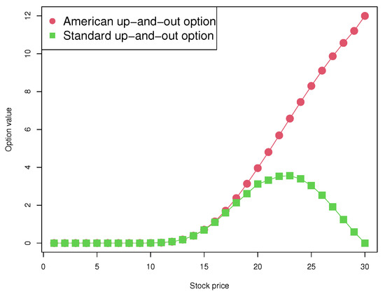
Figure 1. American up-and-out options and standard up-and-out options with different stock prices (r = 0.1).

7. Discussion

Since the operator $Lu$ is not degenerate, the parameter $\epsilon$ is introduced here to establish a regular equation. At the same time, the regular equation incorporates a penalty function controlled by $\epsilon$ to simulate the variation-inequality problem. Based on this regular equation, the existence of weak solutions is analyzed. As for the uniqueness of the solution, the absolute value of the difference between two weak solutions is estimated. It is proved that there is no difference between the two weak solutions by eliminating some non-negative terms.

Analyzing the advantages and disadvantages of this paper, the authors in [4] analyze some theoretical results such as the existence and uniqueness of solution to variation-inequality problems. An advantage of [4] is that it incorporates a nonlinear term behind the degenerate parabolic operator in the form of linear addition. Since the nonlinear term is coupled in a linear way, the author can easily use inequality technique to estimate, and then obtain the relevant results of weak solutions. The variation-inequality problem under degenerate parabolic operators is considered in [6,7]. In [6,7], the authors used second-order degenerate parabolic operators, while this paper used the fourth-order degenerate parabolic operator coupled with a distance function.

8. Conclusions

In the current study, we study an initial boundary value problem variation-inequality

$$\left\{\begin{array}{c}min\{Lu,u-u_0\}=0,(x,t)\in Q_T,\hfill \\ u(0,x)=u_0\left(x\right),x\in \mathsf{\Omega },\hfill \\ u(t,x)=0,(x,t)\in \mathsf{\partial }\mathsf{\Omega }\times (0,T),\hfill \end{array}\right.$$

structured by the following 4th-order degenerate parabolic operators,

$$Lu=\mathsf{\partial }u+\Delta ({\rho }^{\alpha }\left(u\right){\left|\Delta u\right|}^{p-2}\Delta u).$$

In this paper, some theoretical results of weak solutions are given, including the existence and uniqueness. This paper also has some shortcomings: when $p<2$, the result of Lemma 4 cannot be obtained. In addition, if $1<p<2$, scholars analyze the existence of weak solutions when they study the initial boundary value problems of parabolic equations. We will try to analyze the variation-inequality problem in this case.

References

- Chen, X.; Yi, F.; Wang, L. American lookback option with fixed strike price 2-D parabolic variational inequality. J. Differ. Equ. 2011, 251, 3063–3089. [Google Scholar] [CrossRef][Green Version]
- Zhou, Y.; Yi, F. A free boundary problem arising from pricing convertible bond. Appl. Anal. 2010, 89, 307–323. [Google Scholar] [CrossRef]
- Chen, X.; Yi, F. Parabolic variational inequality with parameter and gradient constraints. J. Math. Anal. Appl. 2012, 385, 928–946. [Google Scholar] [CrossRef]
- Sun, Y.; Shi, Y.; Gu, X. An integro-differential parabolic variational inequality arising from the valuation of double barrier American option. J. Syst. Sci. Complex. 2014, 27, 276–288. [Google Scholar] [CrossRef]
- Oaxaca-Adams, G.; Villafuerte-Segura, R.; Aguirre-Hernandez, B. On non-fragility of controllers for time delay systems. A numerical approach. J. Franklin Inst. 2021, 358, 4671–4686. [Google Scholar] [CrossRef]
- López-Rentería, J.A.; Aguirre-Hernandez, B.; Fernandez-Anaya, G. A new guardian map and boundary theorems applied to the stabilization of initialized fractional control systems. Math. Method Appl. Sci. 2022, 38, 1–13. [Google Scholar] [CrossRef]
- Ito, K.; Kunisch, K. Parabolic variational inequalities: The Lagrange multiplier approach. J. Math. Pure Appl. 2006, 85, 415–449. [Google Scholar] [CrossRef]
- Karatzas, I.; Shreve, S.E. Methods of Mathematical Finance; Springer: Berlin/Heidelberg, Germany, 1998. [Google Scholar] [CrossRef]
- Ullah, H.; Adil Khan, M.; Saeed, T. Determination of Bounds for the Jensen Gap and Its Applications. Mathematics 2021, 23, 3132. [Google Scholar] [CrossRef]
- Chen, T.; Huang, N.; Li, X.; Zou, Y. A new class of differential nonlinear system involving parabolic variational and history-dependent hemi-variational inequalities arising in contact mechanics. Commun. Nonlinear Sci. Numer. Simulat. 2021, 101, 1–24. [Google Scholar] [CrossRef]
- Dabaghi, J.; Martin, V.; Vohralik, M. A posteriori estimates distinguishing the error components and adaptive stopping criteria for numerical approximations of parabolic variational inequalities. Comput. Method Appl. Mech. 2020, 367, 113105–113137. [Google Scholar] [CrossRef]
- Zhou, W.; Wu, Z. Some results on a class of degenerate parabolic equations not in divergence form. Nonlinear Anal. Theory Methods Appl. 2005, 60, 863–886. [Google Scholar] [CrossRef]
- Guo, B.; Gao, W. Study of weak solutions for parabolic equations with nonstandard growth conditions. J. Math. Anal. Appl. 2011, 374, 374–384. [Google Scholar] [CrossRef]
Publisher’s Note: MDPI stays neutral with regard to jurisdictional claims in published maps and institutional affiliations. |
© 2022 by the authors. Licensee MDPI, Basel, Switzerland. This article is an open access article distributed under the terms and conditions of the Creative Commons Attribution (CC BY) license (https://creativecommons.org/licenses/by/4.0/).