1. Introduction
There is a large interest in the world research society in the security and ways of its realization in both hardware and software engineering. Nowadays, all areas of IT need to be protected from cyberattacks; some attacks are presented in [
1,
2,
3,
4,
5,
6]. Building secure software on many levels, such as network, application, etc., gave protection from variable attacks and increased level of confidence. To protect all layers of systems can be used ciphers [
7,
8,
9] and/or error-detecting/error-correcting codes, some of them are based on random numbers. For an example, random numbers used in PIN and password generation (PIN Protection Principles, ANSI X9.8:1, Password Generation, FIPS 181-1993), and prime generation (DSA, ANSI X9.30, RSA, ANSI X9.31, Prime Number Generation, ANSI X9.80) random challenges for authentication (Entity Authentication using PKC, FIPS 196) and key confirmation (NIST Key Schemes Recommendation). Such algorithms need to use absolutely random numbers, which are generated by physical processes and then are handled with hardware and software to obtain the correct formal number [
10,
11].
Random numbers are needed in various applications, but finding good random number generators is a difficult task [
11]. All practical methods for generating random numbers are based on deterministic algorithms, so such numbers are more correctly called pseudo-random numbers, since they differ from true random numbers obtained as a result of some natural physical process.
Many systems must have the ability to process the same numbers again under the same conditions and with data of the same origin. For these needs, a pseudorandom generator can be used that can repeat the same numbers as much as it will be needed. There are many examples of using various algorithms, such as linear shift or Yarrow (or Fortuna) [
12], which are very good for their options, and some of them are even cryptographically secure [
13].
Cryptographic applications use deterministic algorithms to generate random numbers, therefore generating a sequence of numbers that theoretically cannot be statistically random. At the same time, if you choose a good algorithm, the resulting numerical sequence—pseudorandom numbers—will pass most tests for randomness. One of the characteristics of such a sequence is a long repetition period [
14].
Examples of well-known cryptographically strong PRNGs are RC4, ISAAC [
15], SEAL [
16], SNOW [
17], the very slow theoretical Bloom–Blum–Shuba algorithm [
18], as well as counters with cryptographic hash functions or cryptographically secure block ciphers instead of the output function.
In addition, cryptographically strong ciphers include generators with multiple shift registers, generators with nonlinear transformations, and majority encryption generators such as .
Many researchers are focusing now on the creation of PRNG based on physical processes, some latest results in this area can be found in [
19,
20,
21], the authors present PRNG based on a discrete hyper-chaotic system with an embedded cross-coupled topological structure, Hopfield Neural Network, and memristive Hopfield neural network (MHNN).
In 2022, the first PRNG algorithm based on the absolute value function Itamaracá [
22] was presented; it is also a simple and fast model that generates aperiodic sequences of random numbers.
In this paper, we present a new algorithm for generating pseudorandom numbers, based on cellular automata, and illustrate its implementation on FPGA and CUDA. Nowadays, there are a number of PRNG algorithms based on CA using one or more rules on the same grid with standard neighborhood patterns, using LFSR, gaps, delays, and, less commonly, nonlinear functions. In this work, the application of several neighborhood templates, several independent cellular automata, and implementation of transitions of various cellular automata according to various sets of rules and expansion of rule sets based on the complementarity of the number of ones and zeros for a statistically normal distribution will be used.
The paper describes in detail the principle of operation of the presented algorithm, its strictly formalized mathematical model, the properties used in the development and the mathematical models and concepts underlying the generator. The paper also contains a description of the tests performed from the ready-made statistical software package, the grounds for these tests, a description of each of them, and the results and performance of the algorithm on the selected tests.
Compared to the existing algorithm, the presented algorithm is different from the previous and similar ones in several respects:
better results in some NIST test;
work speed;
parallelization in hardware implementation;
flexibility;
simplicity of architecture.
The paper is organized as follows:
Section 1 presents an overview of ideas used in random number generators, the mathematical structure of homogeneous structures (HS) and cellular automata,
Section 2 illustrates the created algorithm, giving a mathematical explanation of the presented algorithm,
Section 3 demonstrates test results,
Section 4 illustrates the implementation of the created algorithm on FPGA, and
Section 5 gives CPU and CUDA implementation of the algorithm. In conclusion, a short overview of the presented work is given.
2. Random Number Generators Overview
Random numbers are needed in a variety of applications, yet finding good random number generators (RNG) is a difficult task. In recent years, some new results of building pseudorandom number generators (PRNGs) based on chaos and chaotic map were presented [
23,
24,
25,
26,
27] and in work [
28].
Actually, ’true’ random generation is mostly based on some kind of natural physical processes, or in another way, the ’noise’ source features of some machine hardware may be used. Simplifying, there are many ways to determine some noises as “1” or “0”, giving a sequence of bits, and as a result a number. This number is exactly what we need.
However, the difference between these and pseudorandom generators is in uniqueness, which means that there is no chance of obtaining the same number more than once. The great part of computations where a random number should be used is related to cryptography. For simplicity, there is a need to control the calculation of the speed, effectiveness, and repetition generated numbers (PRNG). Some examples to understand the general idea of such generators will be presented in the following:
There exist many ways to generate pseudorandom numbers on a computer; the most popular one is the Linear Congruential Generator (LCG). In 1951, Lehmer generator [
29] was published, and LCG was published in 1958 [
30,
31]. Today, LCG can be called the method most commonly used for generating pseudorandom numbers. An advantage of LCGs is that the period is known and long with the appropriate parameters. Although not the only criterion, a short period is a fatal flaw in a PRNG [
32]. LCGs based on the following recurrent formula:
The value
m is the module,
a is the multiplier, and
c is an additive constant. The sequence has a maximum possible period
m, after which it starts to repeat itself [
32]. LCGs are very popular among researchers, and most mathematical software packages include them. So-called lagged Fibonacci generators are also widely used. They are of the form:
The numbers
r and
p are called “lags”, and there are methods to choose them appropriately. The operator ∘ can be one of the following binary operators: addition, subtraction, multiplication, or exclusive or. However, it should be noted that, from the point of view of hardware implementation, both congruential and lagged Fibonacci RNGs are not very suitable: they are inefficient in terms of silicon area and time when applied to fine-grained massively parallel machines, for built-in self-test or for other on-board applications [
33].
There is a sufficiently large roadmap to achieve the PRNG objective, which has features such as simplicity, velocity, and unpredictability.
3. Homogeneous Structures (HS) and Cellular Automata (CA)
Homogeneous structures (HS) [
34] may be formally described as
, where
—set of
k-dimensional vectors,
—set of states of one cell in
,
—neighborhood template (ordered set of distinct
k-dimensional vectors from
),
,
—local transition function
.
From the definition of HS, it can be seen that HS can be compared to the set of ordinary Moore automata [
35] if their states depended on the states of neighboring countries. Actually, the neighborhood scheme can differ from each other (Neuman’s scheme is more like a symbol plus with the changeable central cell, Moore’s scheme is more like the square 3 × 3). There are a great number of combinations that can be used.
In this paper, only one class of HS will be used. It can be represented like , where k and n are described above, and m is the set of . Another value needs to be determined—. However, with some restrictions for values , it is obvious that .
Actually, as a result of some HS, without loss of generality for this research, this object can be replaced by CA. Cellular automata (CA) [
34] are dynamical systems in which space and time are discrete. A cellular automata consists of an array of cells, each of which can be in one of a finite number of possible states, updated synchronously in discrete time steps, according to a local, identical interaction rule. Here, we will only consider Boolean automata for which the cellular state
. The state of a cell at the next time step is determined by the current states of the surrounding neighborhood of cells. Cellular array (grid) is
d-dimensional, where
is used in practice; as an example for simplicity of understanding, we shall concentrate on
, i.e., one-dimensional grids.
Each rule in every single cell can be represented as a simple finite automata (or finite-state machine) with its input states, transition function, and output state, which is the result of using the rule function with input state as an entry [
36,
37]. However, in terms of cellular automata, there is an entry as a set of states, called neighborhood, when the next state is in formal dependence of states of the particular target cell and its surrounding cells’ states [
38,
39]. For one-dimensional CA (
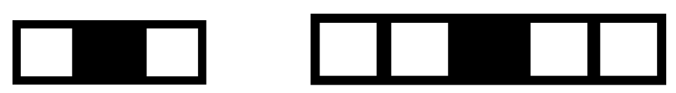
Figure 1), the target cell is surrounded by
r neighbors (cells) at a discrete moment on the appropriate side (by template) where
r cells are called radius (each cell has
cells, which impact its next state).
Besides one-dimensional CAs, there are two main templates for two-dimensional CAs (
Figure 2): the first is the so-called von Neumann neighborhood [
40] (when the target cell is surrounded by four nondiagonal cells) and the second is called the Moore neighborhood [
41] (when the target cell is surrounded by eight cells).
There are also two types of automata, which differ from each other by some kind of complexity in terms of rules. The fact is that one type, called uniform CA, determines one rule for all cells in the grid, but the second type, non-uniform [
42] or inhomogenous may have different rules for cells. At the same time, they both have the same features of simplicity, locality, and parallelism with the difference in realization (inhomogenous ones require more memory sources for describing rules). Additionally, when we think of finite grid of CAs, it should be highlighted that one-dimensional CAs grids are represented by the circular structure, when two-dimensional ones have a grid in toroidal form.
According to Wolfram’s notation [
43], firstly, it should be determined that the configuration is the set of ones and zeros (two-state CA, where the sequence is considered as a random number) at a particular discrete moment of time. Wolfram also suggested additional rule numbers. Let us describe the most popular Wolfram’s
Rule 30 as an example:
In Boolean form,
Rule 30 can be written as
where the radius is
and
is the state of cell
i at time
t. As we can see from this formula,
is the next state of the cell
i at
step, which is a simple Boolean function of neighbor cells states and target cell state at the step
t. That is how a random sequence of bits is obtained, counting every cell as a target cell in the same moment for all the cells. There are several ways to make the sequence more complex and unpredictable, e.g., time spacing and site spacing.
Time spacing is a method of generating configurations, when not every configuration is a part of the resulting sequence; this means that some configurations are generated to produce new ones only, but it will not be in the resulting sequence.
Site spacing is a method of generating sequences when only particular cells’ states in the whole configuration (or a row) are bits of the resulting sequence. These methods are obviously empowered by unpredictability feature for whole sequences, but, of course, time or memory sources with these methods remain the same.
Another example in order to show how Wolfram’s rules can be encoded. For an example: , is denoted Rule 184.
As an example of non-uniform CA, two rules can be taken:
Rule 90 and
Rule 150, which are rules for particular cells in the grid. In Boolean form, the
Rule 90 can be written as
and
Rule 150:
These rules perform a sufficiently effective random number generator, in spite of the fact that they can be simply described as linear Boolean functions.
4. Algorithm of Generating Pseudorandom Numbers on Cellular Automata
The main idea of the presented algorithm is to combine the best practices for generating pseudorandom numbers by cellular automata and a number of improvements to enforce the general features of cellular automata, saving the best.
Figure 3 presents the flowchart of the proposed algorithm.
There are several subsections, which describe step-by-step all levels of algorithm evolution. In addition, there are some ideas for improving the presented algorithm with the help of genetic algorithms to expand the set of rules to be used to generate a pseudorandom number.
4.1. Grid
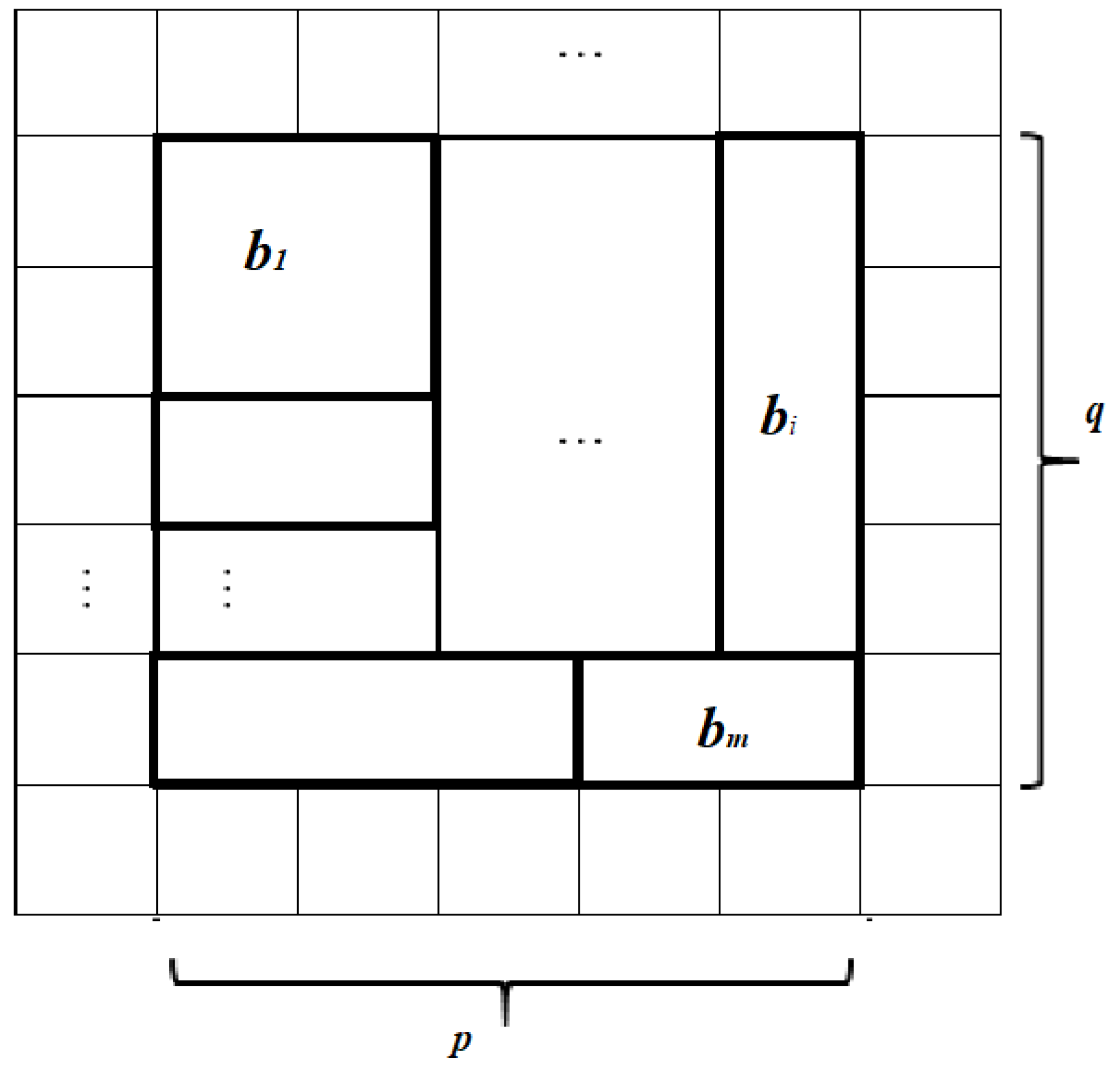
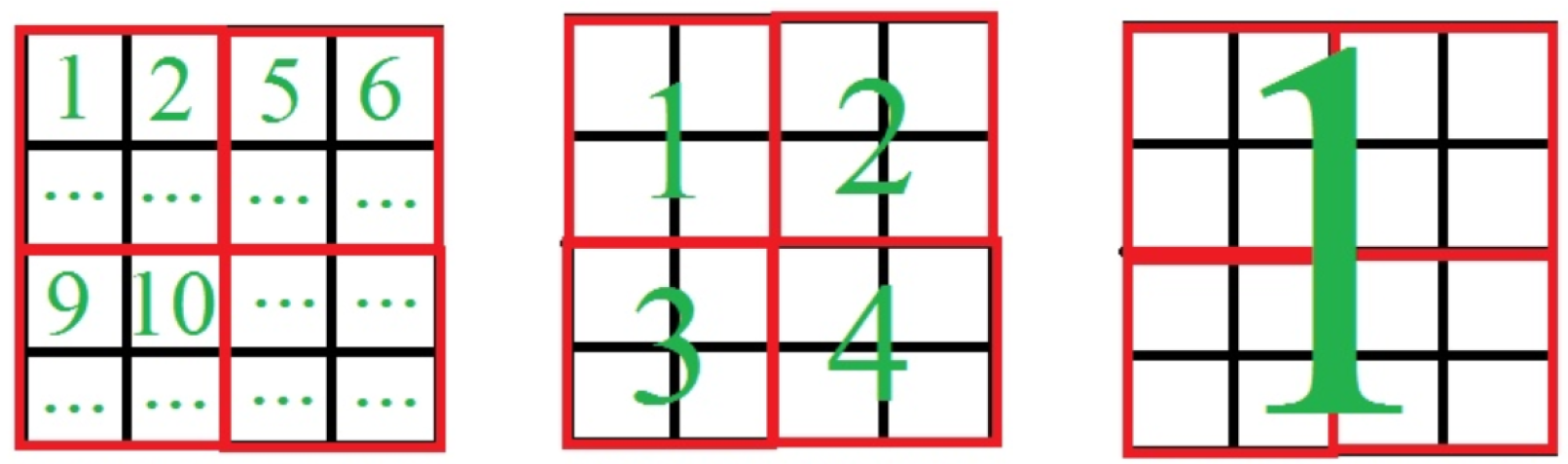
The main result of the presented algorithm is that it can generate pseudo-random sequences of numbers. Despite the fact that CA had already been used in such a way, we improved some characteristics by adding new conditions and ideas. There is a grid, where each cell only has two states: 0 and 1, and states are changed by some function. The result of steps in algorithm will be a binary performed number, which can be formed from the grid (or part of it). Thus, we have a grid with its sizes:
p and
q, which are both prime numbers (to improve periodic features). Changes start right from this stage: dividing all the grid into
blocks, which are formed as rectangles
with sizes
and
, and each block consists of
cells (
Figure 4). Thus, we obtain the equation:
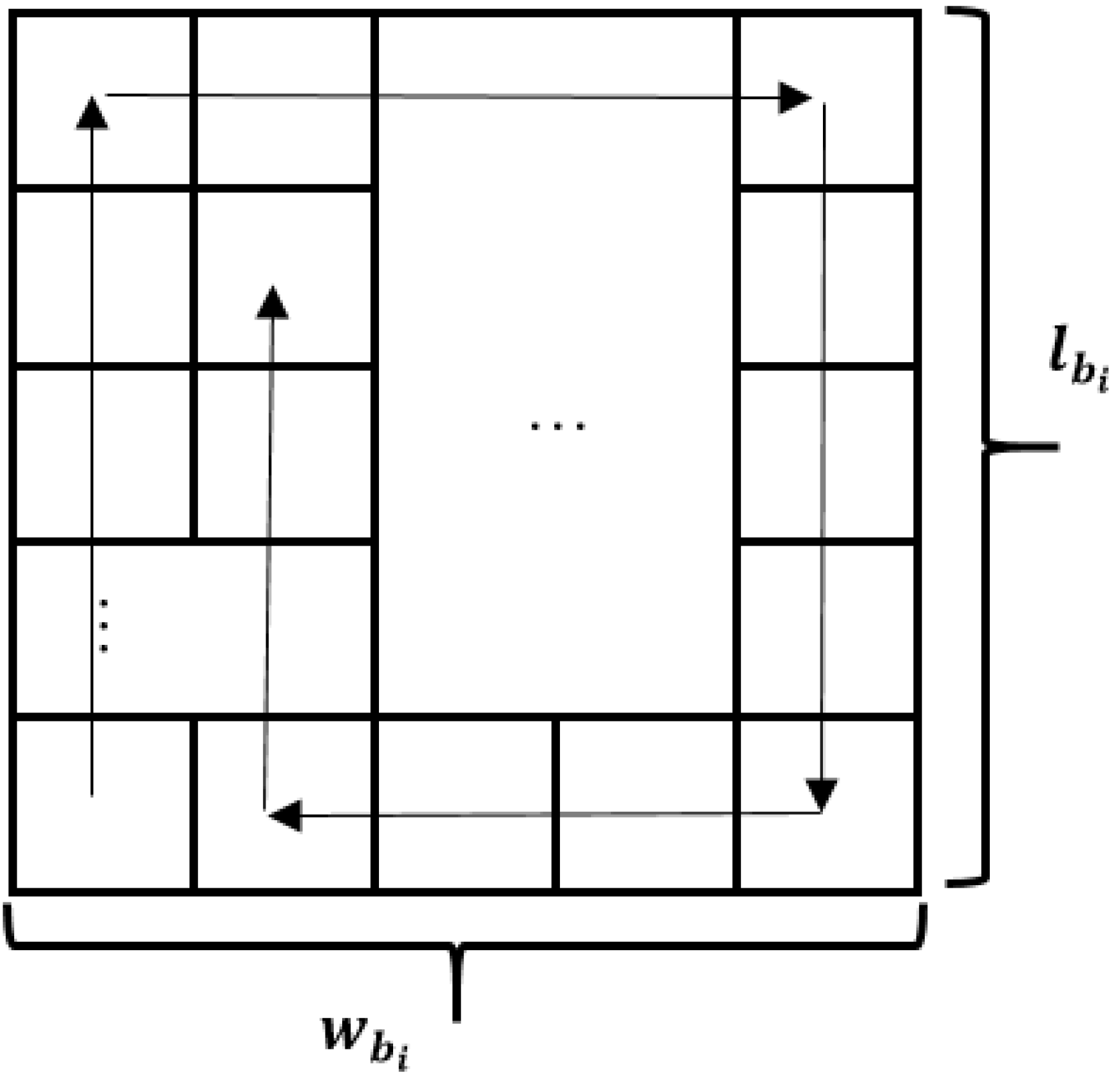
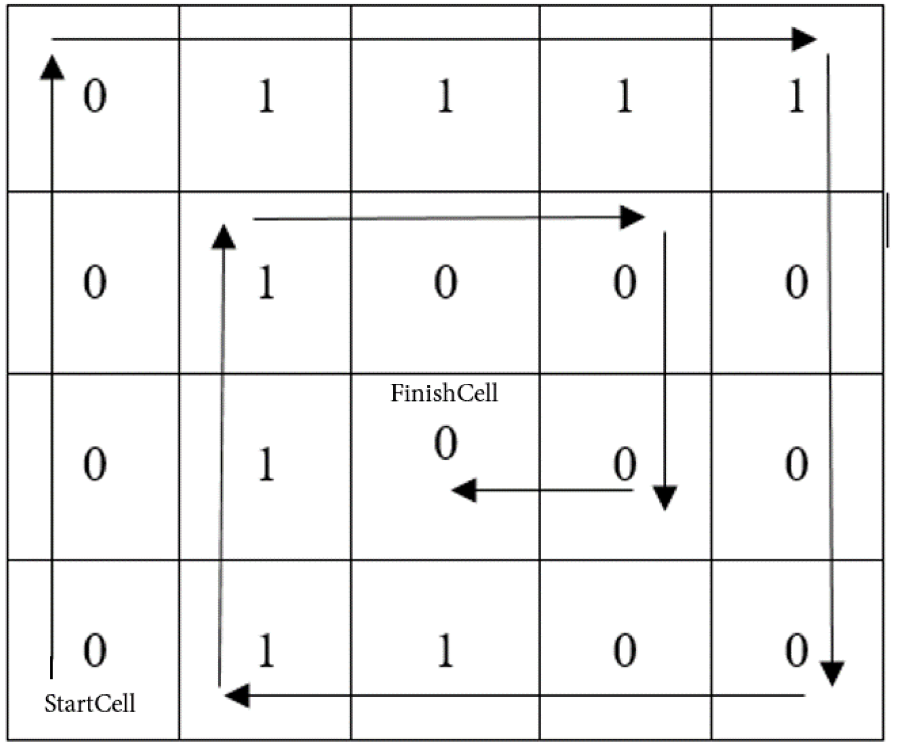
This is quite a simple method, where each block needs to be placed in the grid, called the compass (NESW—North, East, South, West) (
Figure 5). The matter is that there will be a rule by which blocks will be placed from the lower left corner and move to the North (up) till the reaching of edge of the grid or to the next block, then to the East (right), South (down) and West (left), according to their size values. This rule may vary for more flexibility, i.e., “snake” method of filling the grid (filling rows from the bottom to the top with switching to the next row from opposite sides).
Here is an example of using the NESW method of rule. Let us take rule 15 (00001111 in binary representation) and fill the grid with sizes
(
Figure 6).
4.2. Rules and Neighborhood
We will work with only two-dimensional space; this means that we take . Firstly, start configuration will be formed by the rule NESW, the same as blocks. It means that number in binary form will fulfill the blockgrid along the narrowing edges, etc. What about the rules? The solution of this question may be very flexible because the algorithm is provided by two kinds of rules: numbered rules (like the rule 30 at the beginning of this article) and simple operations (their combination). Each block can have its own rule, which makes the whole generating more non-uniform, which leads to unpredictability and better periodic features. Here comes an idea which involves the set of rules in the table, where each rule (both kinds) is encrypted in some combinations, depending on the number of using rules.
Thus, the rule for each block may be chosen by the simple operation from the in case of using every possible rule in the block. However, for the best results, there should be chosen several rules with an equal number of ones and zeros (it may be used for the whole grid—if we have two blocks and three ones in the first block rule, so the second block should have num-3 ones, where num is a length of rule-vector if both vectors are equal). Additionally, to avoid bad generations, we should determine certain rules for the grid. In addition, we could fill the “space” between the actual size of the grid and formal. In order to avoid collisions of values, we should make our grid less than its actual size for one cell (or two, depending on the neighborhood template) on each side.
The last question in generating our pseudorandom numbers is a neighborhood. The fact is that, as far as we have blocks, we can choose several samples for some blocks and its number and variety depending on the number of blocks. We can not use a number of rules more than the number of blocks, but we can use similar ones for several blocks.
4.3. “Repeat Please”
Pseudorandom number generator must have the option of repeating the algorithm in order to obtain a similar number after the same operations with the same conditions and configurations. Actually, not to pass the result number, we can only send the key
K—the sequence of our data in order to repeat operations on the other end, if needed. We use symbol | to mark concatenation:
where
is sent like the sequence of 9 bits where each bit, if it is 1, then cell is in the sample, and, when it is 0, it is out of sample.
| (, 1) | (0, 1) | (1, 1) |
| (, 0) | (0, 0) | (1, 0) |
| (, ) | (, 0) | (1, ) |
Therefore, this neighborhood mapping table becomes such a string
Here are the numbers of coordinates, instead of which, it should be placed 1 or 0. T is a table, where each using rule may be encrypted, for example, a basic binary number. Thus, in spite of the fact that we must send such a long-sized key, we can put some data in the boundary cells, placed around our main grid in order to save correct transition of state. We can save part of the key in these cells, depending on its complexity and size.
4.4. Additional Function
To be sure that our algorithm will generate high-quality random number sequences, we decided to use some nonlinear functions at this level of the development algorithm. The reason is in the CA rules. The fact is that only part of the rules has good random features (the ability to generate complex structures). However, if we take only this part of the rules, we obtain too small a set of needed ones, and there are two ways to improve it. The first one is to add a nonlinear function for XOR with the subset of the grid for making it more complex. The second is that we can choose “good” (having randomness features) packs of rules with the help of genetic algorithms or some kind of tutor algorithm. Therefore, the evolution of CAs will show us only those rules which can be used in practice.
5. Test Results
Our algorithm was tested with the help of the NIST Test Suite, which was developed to test RNG and PRNG [
44]. The process of the test involved: generation sequences of bits by our algorithm (around 1,000,000 bits), testing.txt file with a sequence with an NIST test suite. The 10,000 variations of the rules pack and ways of filling the grid were tested, as sizes of grids. As a result, the number of the most “productive” packs of rules-grid size-neighborhood were highlighted.
Thus, we used the grid with sizes , divided by six blocks of approximately equal lengths, while the width of each block was 53. Each block was filled with bits, generated by results of multiplication of blocks’ sizes, with the NESW method. The neighborhood template was simple and even classical enough; it was a 3B rule (center cell change state in dependence of its previous state and left and right neighbors’ ones). The package of rules was: {45, 75, 89, 101, 135, 86}.
Rule 45:
| 000 | 001 | 010 | 011 | 100 | 101 | 110 | 111 |
| 1 | 0 | 1 | 1 | 0 | 1 | 0 | 0 |
Rule 75:
| 000 | 001 | 010 | 011 | 100 | 101 | 110 | 111 |
| 1 | 1 | 0 | 1 | 0 | 0 | 1 | 0 |
Rule 89:
| 000 | 001 | 010 | 011 | 100 | 101 | 110 | 111 |
| 1 | 0 | 0 | 1 | 1 | 0 | 1 | 0 |
Rule 101:
| 000 | 001 | 010 | 011 | 100 | 101 | 110 | 111 |
| 1 | 0 | 1 | 0 | 0 | 1 | 1 | 0 |
Rule 135:
| 000 | 001 | 010 | 011 | 100 | 101 | 110 | 111 |
| 1 | 1 | 1 | 0 | 0 | 0 | 0 | 1 |
Rule 86:
| 000 | 001 | 010 | 011 | 100 | 101 | 110 | 111 |
| 0 | 1 | 1 | 0 | 1 | 0 | 1 | 0 |
5.1. Short Description of Criteria with Results
The test statistic is used to calculate a
p-value that summarizes the strength of the evidence against the null hypothesis. For these tests, each
p-value is the probability that a perfect random number generator would have produced a sequence less random than the sequence that was tested, given the kind of non-randomness assessed by the test. If a
p-value for a test is determined to be equal to 1, then the sequence appears to have perfect randomness. A
p-value of zero indicates that the sequence appears to be completely non-random. A significance level (
) can be chosen for the tests. If
p-value
, then the null hypothesis is accepted; i.e., the sequence appears to be random. If
p-value
, then the null hypothesis is rejected; i.e., the sequence appears to be non-random. The parameter
denotes the probability of the
error (if the data are, in truth, random, then a conclusion to reject the null hypothesis (i.e., conclude that the data are non-random) will occur a small percentage of the time) [
44],
is equal to
[
44].
5.1.1. Frequency (Monobit) Test
The focus of the test is the proportion of zeros and ones for the entire sequence. The purpose of this test is to determine whether the number of ones and zeros in a sequence is approximately the same as would be expected for a truly random sequence. The test assesses the closeness of the fraction of ones to
, that is, the number of ones and zeros in a sequence should be about the same. All subsequent tests depend on the passing of this test [
44].
| p-Value | Proportion | Statistical Test |
| 0.744146 | 99.6% | Frequency |
5.1.2. Frequency Test within a Block
The focus of the test is the proportion of the ones within
M-bit blocks. The purpose of this test is to determine whether the frequency of ones in an
M-bit block is approximately
M/2, as would be expected under an assumption of randomness. For block size
, this test degenerates to the Frequency (monobit) test [
44].
| p-Value | Proportion | Statistical Test |
| 0.380537 | 99.4% | BlockFrequency |
5.1.3. Runs Test
The focus of this test is the total number of runs in the sequence, where a run is an uninterrupted sequence of identical bits. A run of lengths
k consists of exactly
k identical bits and is bounded before and after with a bit of opposite value. The purpose of the run test is to determine whether the number of runs of ones and zeros of various lengths is as expected for a random sequence [
44].
| p-Value | Proportion | Statistical Test |
| 0.428244 | 98.5% | Runs |
5.1.4. Longest Run of Ones in a Block
The focus of the test is the longest run of ones within
M-bit blocks. The purpose of this test is to determine whether the length of the longest run of ones within the tested sequence is consistent with the length of the longest run of ones that would be expected in a random sequence. Note that an irregularity in the expected length of the longest run of ones implies that there is also an irregularity in the expected length of the longest run of zeroes. Therefore, only a test for ones is necessary [
44].
| p-Value | Proportion | Statistical Test |
| 0.383827 | 99.1% | LongestRun |
5.1.5. Rank Test
The focus of the test is the rank of disjoint sub-matrices of the entire sequence. The purpose of the test is to check for linear dependence among fixed length substrings of the original sequence [
44].
| p-Value | Proportion | Statistical Test |
| 0.702458 | 99.0% | Rank |
5.1.6. Discrete Fourier Transform (Spectral) Test
The focus of this test is the peak heights in the Discrete Fourier transform of the sequence. The purpose of this test is to detect periodic features (i.e., repetitive patterns that are close to each other) in the sequence tested that would indicate a deviation from the assumption of randomness. The intention is to detect whether the number of peaks exceeding the 95% threshold is significantly different than 5% [
44].
| p-Value | Proportion | Statistical Test |
| 0.650637 | 99.5% | FFT |
5.1.7. Non-Overlapping Template Matching Test
The focus of this test is the number of occurrences of prespecified target strings. The purpose of this test is to detect generators that produce too many occurrences of a given non-periodic (aperiodic) pattern. For this test and for the Overlapping Template Matching test, an
m-bit window is used to search for a specific
m-bit pattern. If the pattern is not found, the window slides into a bit position. If the pattern is found, the window is reset to the bit after the found pattern and the search is resumed [
44].
| p-Value | Proportion | Statistical Test |
| 0.433358 | 98.7% | NonOverlappingTemplate |
5.1.8. Overlapping Template Matching Test
The focus of the Overlapping Template Matching test is the number of occurrences of prespecified target strings. Both this test and the Non-overlapping Template Matching test use an
m-bit window to search for a specific
m-bit pattern. As in the previous test, if the pattern is not found, the window slides one bit in the position. The difference between this test and the previous test is that; when the pattern is found, the window slides only one bit before resuming the search [
44].
| p-Value | Proportion | Statistical Test |
| 0.632191 | 100% | OverlappingTemplate |
5.1.9. Maurer’s “Universal Statistical Test”
The focus of this test is the number of bits between the matching patterns (a measure that is related to the length of a compressed sequence). The purpose of the test is to detect whether the sequence can be significantly compressed without loss of information. A significantly compressible sequence is considered to be non-random [
44].
| p-Value | Proportion | Statistical Test |
| 0.414862 | 98.3% | Universal |
5.1.10. Linear Complexity Test
The focus of this test is the length of a linear feedback shift register (LFSR). The purpose of this test is to determine whether the sequence is complex enough to be considered random. Random sequences are characterized by longer LFSRs. An LFSR that is too short implies non-randomness [
44].
| p-Value | Proportion | Statistical Test |
| 0.730485 | 100% | LinearComplexity |
5.1.11. Serial Test
The focus of this test is the frequency of all possible overlapping
m-bit patterns throughout the sequence. The purpose of this test is to determine whether the number of occurrences of the
-bit overlapping patterns is approximately the same as would be expected for a random sequence. Random sequences have uniformity; that is, every
m-bit pattern has the same chance of appearing as every other
m-bit pattern [
44].
| p-Value | Proportion | Statistical Test |
| 0.651956 | 99.3% | Serial |
5.1.12. Approximate Entropy Test
The focus of this test is the frequency of all possible overlapping
m-bit patterns across the entire sequence. The purpose of the test is to compare the frequency of overlapping blocks of two consecutive/adjacent lengths (
m and
) against the expected result for a random sequence [
44]:
| p-Value | Proportion | Statistical Test |
| 0.778903 | 99.1% | Approximate Entropy |
5.1.13. Cumulative Sums (Cusums) Test
The focus of this test is the maximal excursion (from zero) of the random walk defined by the cumulative sum of adjusted (−1, +1) digits in the sequence. The purpose of the test is to determine whether the cumulative sum of the partial sequences occurring in the tested sequence is too large or too small relative to the expected behavior of that cumulative sum for random sequences. This cumulative sum may be considered as a random walk. For a random sequence, the excursions of the random walk should be near zero. For certain types of non-random sequences, the excursions of this random walk from zero will be large [
44].
| p-Value | Proportion | Statistical Test |
| 0.734146 | 99.9% | CumulativeSums |
5.1.14. Random Excursions Test
The focus of this test is the number of cycles that have exactly
K visits in a cumulative sum random walk. The cumulative sum random walk is derived from partial sums after the (0, 1) sequence is transferred to the appropriate (
, +1) sequence. A cycle of a random walk consists of a sequence of steps of unit length taken at random that begin at and return to the origin. The purpose of this test is to determine if the number of visits to a particular state within a cycle deviates from what one would expect for a random sequence. This test is actually a series of eight tests (and conclusions), one test (conclusion) for each of the states
,
,
,
, +1, +2, +3, +4 [
44].
| p-Value | Value |
| 0.673779 | |
| 0.640660 | |
| 0.636757 | |
| 0.906842 | |
| 0.614216 | +1 |
| 0.042225 | +2 |
| 0.570447 | +3 |
| 0.802887 | +4 |
5.1.15. Random Excursions Variant Test
The focus of this test is the total number of times a particular state is visited (that is, occurs) in a cumulative sum random walk. The purpose of this test is to detect deviations from the expected number of visits to various states in the random walk. This test is actually a series of 18 tests (and conclusions), one test (conclusion) for each of the states:
…
and +1…+9 [
44].
| p-Value | Value |
| 0.148224 | |
| 0.293802 | |
| 0.799213 | |
| 0.810598 | |
| 0.589138 | |
| 0.525096 | |
| 0.584469 | |
| 0.659030 | |
| 0.878513 | |
| 0.878513 | +1 |
| 0.469278 | +2 |
| 0.502912 | +3 |
| 0.711568 | +4 |
| 0.910749 | +5 |
| 0.860976 | +6 |
| 0.702797 | +7 |
| 0.532906 | +8 |
| 0.543193 | +9 |
The choice of rules is determined by good randomness and an equal number of ones and zeros in each of these particular rules.
Table 1 presents the results of the NIST test suite package [
44] with the input of the file, generated by the developed algorithm.
All p-values in this table are averaged from 10–100 rounds of tests.
In addition, there is a comparison (
Table 2) between the measurements of the NIST test suite of the presented method and the Linear Congruential method, and it is observed that the presented method obtains better results in some tests, and the
p-value in some tests is much higher.
6. FPGA Implementation
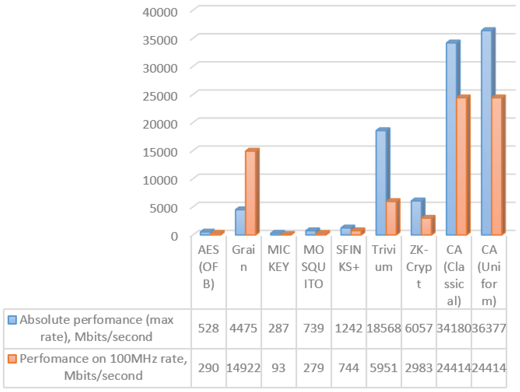
The presented algorithm has two implementations, one on FPGA and one on CUDA. Here, there is a chart (
Figure 7) from the paper [
45], which shows the velocity of a pseudorandom numbers’ generator, based on a cellular automaton implemented on FPGA. There are several algorithms, which were measured on the same FPGA platform from eSTREAM (as pseudorandom generators, which were considered strictly and detailed enough for their process velocity and statistical features) [
46,
47].
Hardware modeling was performed on Artix 7 xc7a200tfbg676-3 in Vivado 2016.3. The synthesis parameters are shown in
Table 3. The modeling results are presented in
Table 4. There are not enough resources of the device for size 1024 on 1024 and 4096 on 4096. Absolute performance of the proposed device is up to 1540 times greater than that of the known devices shown in
Figure 7, and performance at the 100 MHz rate of the proposed device is up to 1074 times higher than that of the known ones.
We can compare the results of the FPGA-based implementation with the results presented in [
48,
49].
7. CUDA Implementation
Hardware used:
CPU: Intel Core i5-4670
GPU: GeForce GTX 750 Ti
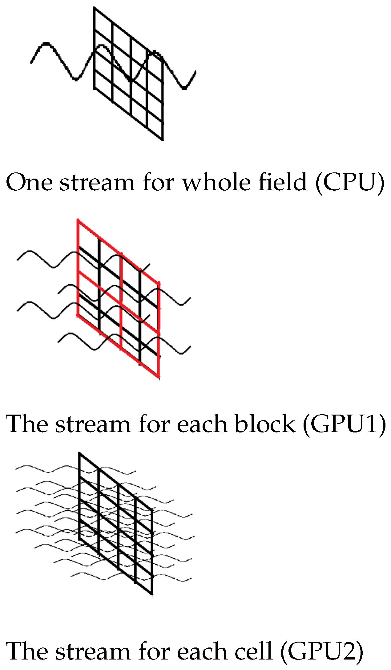
As noted above, one of the main advantages of the method is the possibility of parallelization of the calculations. Here, we will describe the implementation of the algorithm on CUDA (GPU) with the main differences from the CPU variant.
There are two approaches:
Sequential calculation of blocks, parallel calculation of cells in blocks.
The cycle on the CPU is created in which each block will be calculated. To calculate a block on the GPU for each cell, a stream is created and the final state of the cell is calculated.
Parallel computation of blocks, parallel computation of cells in blocks.
Each cell downstream will be run; in each stream, the block to which the cell belongs is determined, and then the final state of the cell is calculated.
The most difficult part in this step is to calculate the index of the cell in the block when it is circled clockwise (NESW). Since the program is executed in parallel, there is no sequential round-trip in a clockwise direction, and the index is calculated using a formula that uses the perimeter of the rectangle.
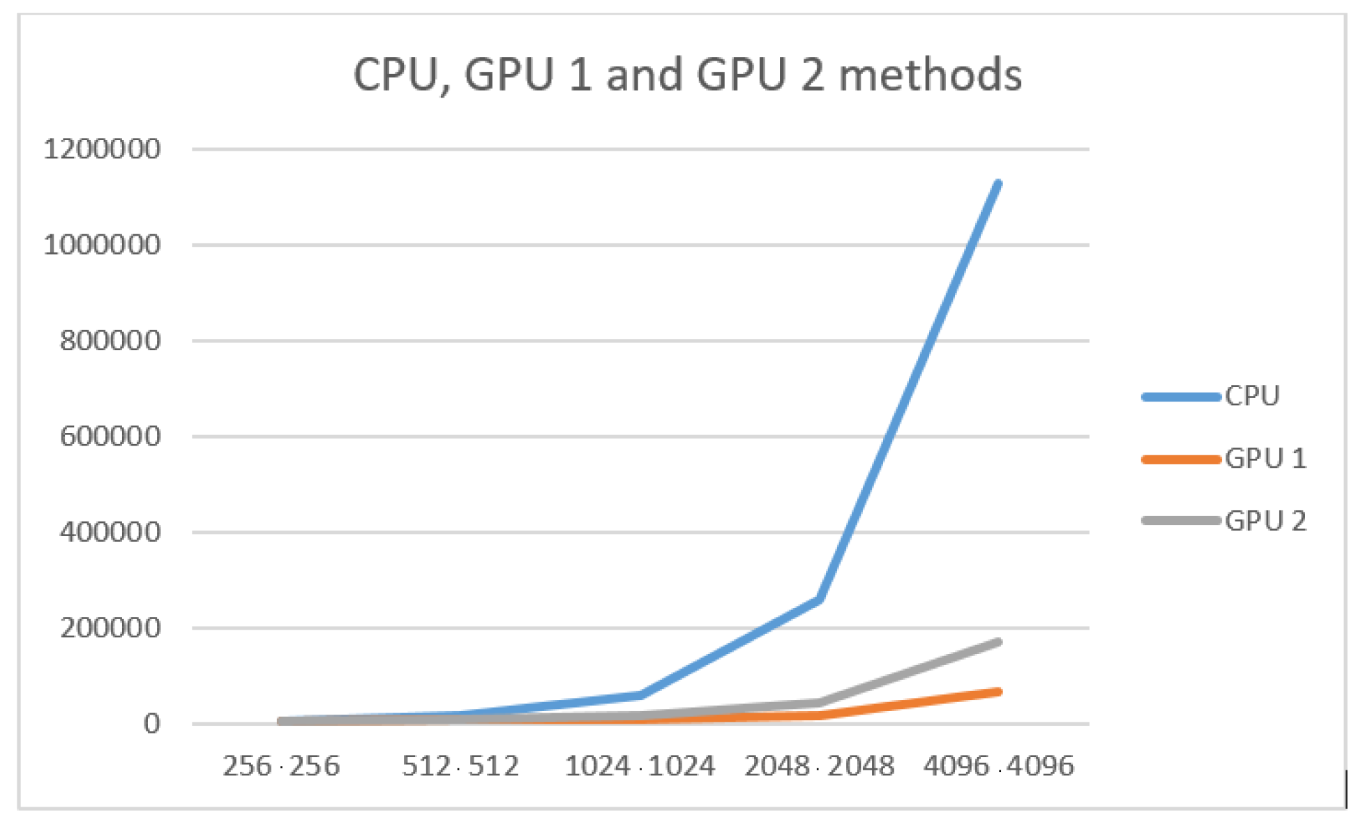
The difference between the three hardware-based methods of the described PRNG implementation can be seen in
Figure 8 and
Figure 9 and
Table 5 presents the comparison between the results of the tests of these three methods. The difference chart is presented in
Figure 10.
After CUDA research, there were several tests with variable block size (
Table 6).
It is obvious that all the advantages and disadvantages of CPU- and GPU-based implementations are concluded. However, it is not in such a way for GPU1 and GPU2 implementations difference.
The main differences between GPU1 and GPU2 implementations are that, in the GPU2 implementation, the calculation of blocks and cells occurs in parallel, and in GPU1—the cells in the block are calculated in parallel, and the blocks are sequential. In the second case, additional calculations are needed, such as the calculation of the cell belonging to the unit. The second implementation will give an increase in performance with a large number of blocks and a large volume of cells.
It can be seen from the tables, on small data, that two implementations on the GPU lose their pros to the CPU. This is because the amount of computation is so small that copying the device into memory and additional computations in each GPU stream take a lot of time for this amount of data.
However, on large amounts of data, implementation on GPU wins due to parallel computing. The use of additional calculations is due to the fact that they are performed in parallel and allow each cell and block to be calculated in parallel.
8. Discussion
It should be noted that, from the point of view of hardware implementation, both linear congruent and retarded Fibonacci generators are not very suitable [
50,
51,
52]: they are not efficient in terms of microprocessors and time, when it is necessary to apply PRNG for distributed machines and parallel computing, for embedded testers, or for other applications at this level.
A third widely used type of generator is the so-called linear feedback generator (LFSR). Linear feedback shift registers are common among physicists and computer engineers. There are forms of LFSR that are suitable for hardware implementation.
However, it turns out that, compared to equivalent CA-based generators, they are less efficient; in addition, they are less applicable in terms of the possibility of implementation and debugging, although the area required for the CA cell is slightly larger than for the LFSR [
38]. In [
53], comparing LFSR and CA, was also illustrated, the benefits of using CA in PRNG were shown.
Moreover, different sequences generated by the same CA are much less correlated than similar sequences generated by LFSR. This means that CA-generated bit sequences can be used in parallel, which implies clear advantages in using them in applications.
PRNG based on CA outperforms similar algorithms in terms of performance characteristics, flexibility in development, scalability and parallelization properties.
9. Conclusions
This paper presents a pseudorandom generating algorithm on CA in a detailed form with new ideas to improve some features of an algorithm, which existed before. Testing results show that the described generator has good perspectives because of its effectiveness, simplicity, velocity, and improved unpredictability.
The proposed PRNG algorithm combines the advantages of the speed of cellular automata on a two-dimensional basis and ease of implementation, as a step-by-step series of Moore automata with initiated initial states. Compared to the classical algorithms generating pseudo-random numbers, the cellular automaton presented algorithm has such changes:
application of several neighborhood templates;
the use of several independent cellular automata;
implementation of transitions of various cellular automata according to various sets of rules;
expansion of rule sets based on the complementarity of the number of ones and zeros for a statistically normal distribution.
The changes mentioned helped our algorithm to obtain better results in some NIST tests compared to existing algorithms. The developed algorithm can be successfully used and implemented in many cryptographic primitives, given the ease of implementation, speed, and compliance with modern development models (parallelization of processes).
Future research will be focusing on an implementation presented generator in different cryptographic applications such as lightweight cryptography or coding theory.


 ,
, 


