Abstract
The model of any epidemic illness is evolved from the current susceptibility. We aim to construct a model, based on the literature, different to the conventional examinations in epidemiology, i.e., what will occur depends on the susceptible cases, which is not always the case; one must consider a model with aspects such as infections, recoveries, deaths, and vaccinated populations. Much of this information may not be available. So without artificially assuming the unknown aspects, we frame a new model known as IVRD. Apart from qualitative evaluation, numerical evaluation has been completed to aid the results. A novel approach of calculating the fundamental reproduction/transmission range is presented, with a view to estimating the largest number of aspects possible, with minimal restrictions on the spread of any disease. An additional novel aspect of this model is that we include vaccines with the actively infected cases, which is not common. A few infections such as rabies, ebola, etc., can apply this model. In general, the concept of symmetry or asymmetry will exist in every epidemic model. This model and method can be applied in scientific research in the fields of epidemic modeling, the medical sciences, virology, and other areas, particularly concerning rabies, ebola, and similar diseases, to show how immunity develops after being infected by these viruses.
Keywords:
new IVRD epidemic model; basic reproduction number; stability analysis; sensitivity analysis; pandemic model; vaccinated cases MSC:
74H15; 34A07
1. Introduction
Nature is miraculous in both positive and negative ways. The negative include disasters, such as volcanoes and earthquakes, and diseases, both curable and incurable. Even curable diseases can be dangerous, since they can be transmitted to a larger community of people through a lack of education about and awareness of a disease, lack of hygiene, etc. When such diseases emerge, they can spread and kill many people who are vulnerable to infection. The role of immunity is predominant in protecting many people; however, when a disease is new, immunity is less common. An immune system may not be effective against a new invader. Meanwhile, incurable diseases are also transmitted; however, medical science is still struggling to cure such diseases as Human Immunodeficiency Virus (HIV) and Acquired Immunodeficiency Syndrome (AIDS). The medical definition of non-accidental death is a factor that ends a human life, which is not a specific disease or symptom for everyone, but differs depending on factors including age, immunity, diseases (both hereditary and nonhereditary), lifestyle, habits, habitats, occupation, etc. Science and inventions will not stop aging or death. In addition, there are many things that are not currently explained by science. One such thing is the study of an epidemic model without susceptible cases. From the very first epidemic model until now, for example, the Kermack–McKendrick SIR Model, most mathematicians have not considered an epidemic model without susceptibility. Prasantha Bharathi et al. [1] studied the spread of COVID-19 without susceptible cases, which matched the biological ratios very closely. Motivated by that study, we would like to frame a general epidemic model, which includes vaccinated and death cases in addition to infected and recovered cases.
Modeling in mathematics has been used to support community intervention and social distancing measures during the COVID-19 pandemic. Before the pandemic, models were used to identify critical situations and plan actions in case of emergencies. When a pandemic begins, policy makers use mathematical models to determine (a) when and where the pandemic began, (b) the risk of spread to a particular region, (c) the risk of export to other regions, and (d) the epidemiologic characteristics. In this context, researchers use more areas of analysis to monitor infectious diseases, including control strategies, prediction of various indicators related to infectious diseases (mortality, hospitalization, and morbidity), optimal allocation of medical resources in the fight against disease, explanation of human behavior during disease pandemics, and openness to public policy. After an epidemic, mathematical models are used to propose solutions for recovery and mitigation of the long-term negative effects of an epidemic. As noted above, the concept of symmetry can be adapted to every epidemic model, for example, patchy epidemic environments, itinerant population exchange matrices, epidemic models describing networks, and time-invariant epidemic model parameterizations, among others; see details in [2] and references therein. Moreover, see [3] for verification of the behavior of the model with susceptible and exposed populations. Some of the works that motivated this present research include a heat transfer model developed using a fractional derivative [4], the use of the Laplace Adomian Decomposition method (LADM) to analyze an SEIR model for the first time [5], a COVID-19 model using the fractional derivative [6], research into the existence and uniqueness of nonlinear epidemiology applications [7], an SEIR model using vaccination strategy and a fractional order [8], a COVID-19 model under the lockdown strategy [9], an SIR model following the social distancing strategy [10], an Indonesian SIR COVID-19 epidemic fuzzy model [11], a Stiff Fuzzy COVID-19 model under the 14-day transmission model [1], a new fractional epidemic model dealing with a death population [12], as well as an LADM for solving a model for HIV infection of cells [13], a fractional SEIQ with delay [14], a fractional model of dengue transmission [15], and a discrete COVID-19 stochastic model [16]. Recently, authors including Mathews, Vitaly, and many others [17,18,19,20,21,22,23,24,25] have started to work on epidemic modeling, especially on models for COVID-19.
2. IVRD Epidemic Model Formulation
First, let us discuss the reason for the following type of novel model, i.e., . In a few cases, vaccines can be used to deal with live viral infections. The idea is to enhance immunity by offering a vaccination that mimics the signs and symptoms of the infectious disease, for example, rabies, a risky neurological ailment.
Usually, rabies spreads via the saliva of an animal, mainly a mammal, infected with the disease. It can take up to 2 or 3 weeks for rabies to actively cause infection in a human. Medically speaking, a person is suspected to have rabies when bitten by an animal that may have rabies. The person may also begin to have signs and symptoms. From the signs, symptoms, and a lab report, the infection can be confirmed. This duration of 2 or 3 weeks of infection time is sufficient for vaccination.
The vaccine is given to an actively infected individual to enhance the immune reaction and keep the virus from penetrating the nerve tissue. Thus, vaccination during the actively infectious period of rabies prevents the damaging neurological outcomes of the disease. First, the person will recover from the symptoms and then the infection. An identical method is carried out for Ebola, which is regarded as one of the fastest spreading and deadliest viruses on the planet. The illness is transmitted by animals such as bats and monkeys and causes the death of 80% of those infected within weeks. Its vaccine enhances the immune system of those infected, to prevent many of them from dying.
Let us use the following considerations to build the desired mathematical model (see Table 1, and Figure 1).

Table 1.
Symbols and Descriptions.
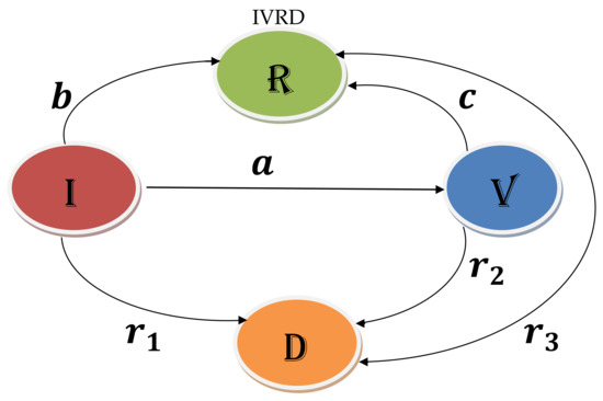
Figure 1.
Model Formulation.
3. Preliminaries
We provide some necessary results of fractional differential equations.
Definition 1.
From [4], the ABC fractional derivative for any function f over the interval is defined as
where is a normalized function satisfying , and has the same properties as in the Caputo and Fabrizio case [26].
Definition 2.
From [4], the Laplace transformation of the ABC derivative is developed as , where .
Definition 3.
[4] The Atangana–Balenanu integral of the function having order is defined as
Moreover, when , the classical integral is obtained.
The initial conditions menttioned in Table 1 are satisfied; therefore, the total population of size N becomes constant. . Although there are few problems with initializations on the ABC operator, we prefer to model any classical time-derivative dynamical system using this operator, as it combines both nonlocal and nonsingular kernels in its formulation.
Here, we present an important aspect of using differential equations over discrete populations (see Figure 1). The problem is that we can use difference equations to solve small populations; however, when large populations are considered, differential equations are preferred to avoid the chaotic behavior that arises in the difference equation, as one can see in the large-population discrete-population logistic growth model by means of difference equations. Moreover, when the differential equation is applied, there is a significant process that permits one to analyze some of the characteristics of the system such as equilibrium points, the stability and positivity of the solutions, etc.
4. Equilibrium and Stability and Positivity Analysis
4.1. Equilibrium Points
In the system (2), we consider , , and Then, the disease-free equilibrium points are either . The disease-dependent equilibrium points are given by , i.e.,
i.e., the disease-dependent equilibrium points are calculated as
4.2. Basic Transmission Number: -Estimation
Let be the basic transmission number. Since we are not aware of the susceptible populations, we need to impose a new technique, following Prasantha Bharathi et al. [1]. We need to bear in mind that the infected population is already infected and is not being infected by others; the dead population is also not being infected, and the vaccinated infected population is being infected until they are completely recovered. The only case free from infection and possible secondary infection due to transmission is the recovered population R, as far as the IVRD population is concerned. So, we use the new formula to estimate the lower and upper limit and the upper limit
where can be calculated with the support of . We then obtain . Then, we arrive at . We found that , and the basic transmission limit is given by , which is approximately .
Theorem 1.
The mathematical model that we considered (2) will be estimated as locally asymptotically stable when the real parts of all the roots (eigenvalues) of the characteristic polynomial hold only negative values.
Proof.
We now linearize (2) formed by the aid of the initial populations, which appears to be the Jacobian matrix form, J
The characteristic polynomial of the above matrix at was found to be
On solving the above polynomial by taking
we obtain the eigenvalues as
For the system (2), since the four roots or eigenvalues of the characteristic polynomial of the system have only negative real parts, we can see that the system is locally asymptotically stable for the initial populations. □
5. Existence of the Positivity of the Solutions
Theorem 2.
For the time , the solution path traced by our IVRD model (2) is positively bounded for all positive initial conditions at any time t.
Proof.
From (2), we take
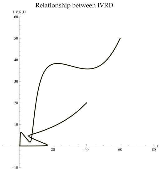
On solving the system of Equation (2), we find their exact solutions. We present the parametric plot of Since the system is nonlinear, it was not easy to estimate it appropriately. However, we can present the structure of the exact solutions of those parameters. We obtained the solutions of and as follows.
We know that the total population is the sum of all cases, i.e.,
which implies Hence, the total population is always positive at any time (see, Figure 2).
Figure 2.
Parametric Plot.
Hence, the proof. □
6. Numerical Simulations
In this section, the values obtained for , , , and are plotted, and the description of the figure is presented in the Discussion and Conclusions Section. The stability and convergence of methods such as the Laplace Adomian Decomposition method and the Differential Transform method have been studied in Sabir Widatalla and Ahmad et al. in [27,28], respectively. Since we concentrate more on the numerical solution, we recommend the reader to see the details of the convergence and stability of the model in the above papers.
For , , , , and at , refer to the Table 2, Figure 3, Figure 4, Figure 5, Figure 6 and Figure 7, and for for various values of t, refer to Figure 8, Figure 9, Figure 10, Figure 11, Figure 12, Figure 13, Figure 14, Figure 15, Figure 16, Figure 17, Figure 18 and Figure 19.
Table 2.
IVRD at .
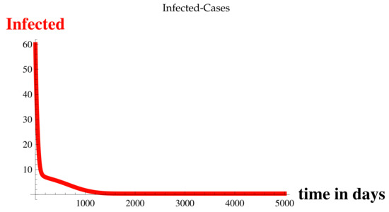
Figure 3.
Infected Cases at .
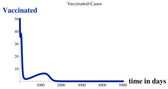
Figure 4.
Vaccinated Cases at .
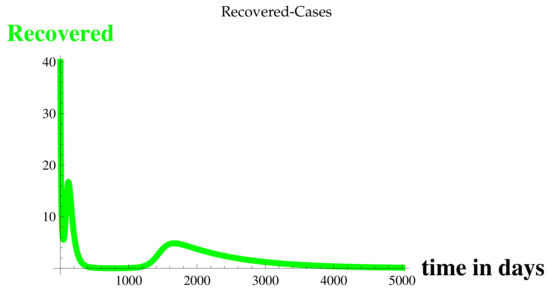
Figure 5.
Recovered Cases at .
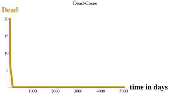
Figure 6.
Dead Cases at .
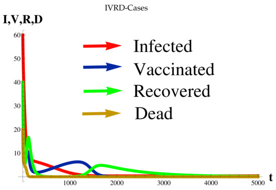
Figure 7.
at .
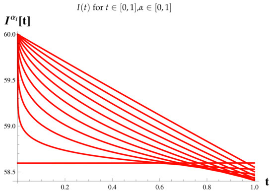
Figure 8.
Fractional Model: Infected Cases.
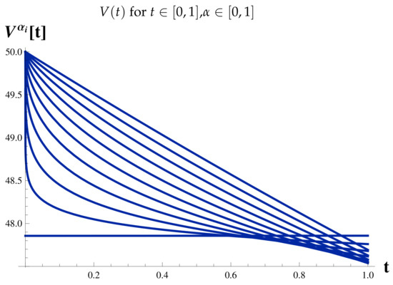
Figure 9.
Fractional Model: Vaccinated Cases.
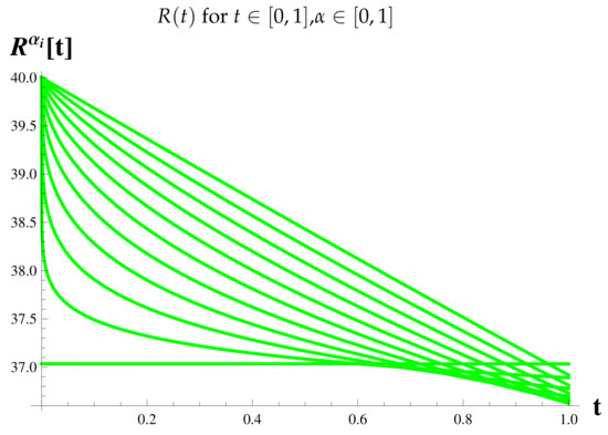
Figure 10.
Fractional Model: Recovered Cases.
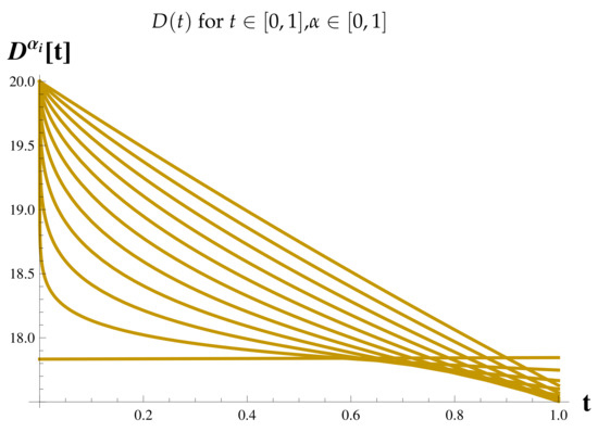
Figure 11.
Fractional Model: Dead Cases.
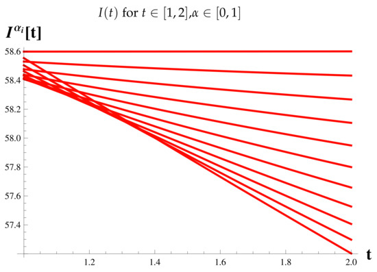
Figure 12.
Infected Cases at .
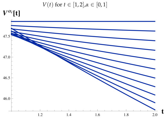
Figure 13.
Vaccinated Cases at .
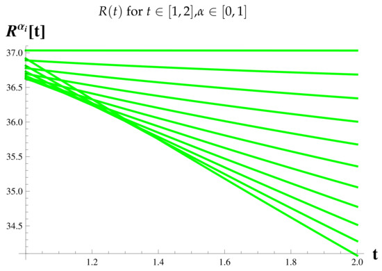
Figure 14.
Recovered Cases at .
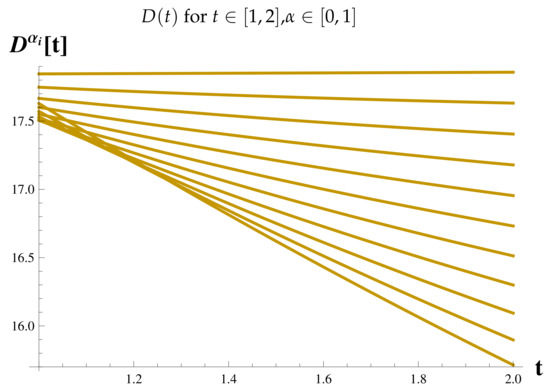
Figure 15.
Dead Cases at .
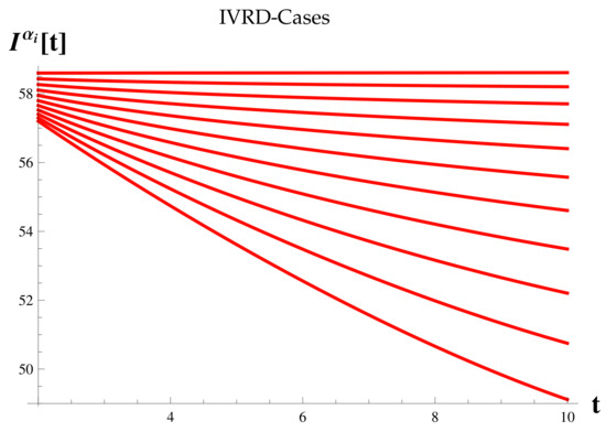
Figure 16.
Infected Cases at .
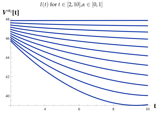
Figure 17.
Vaccinated Cases at .
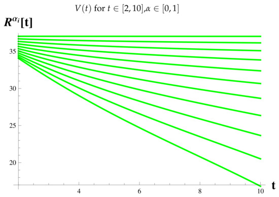
Figure 18.
Recovered Cases at .
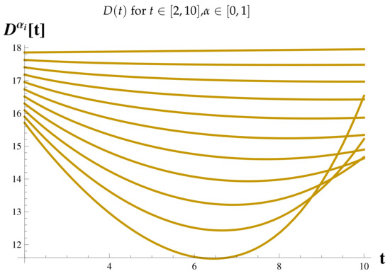
Figure 19.
Dead Cases at .
Figure 7 shows the relationship between the timing of the rise and fall of each set of cases.
6.1. Laplace Adomian Decomposition Method (LADM)
Similar to [5], we use the LADM, and the values of , , , and are found by the procedure given below.
where and are the Adomian polynomials defined by
i.e.,
and so on.
and so on.
and so on.
and so on.
and so on.
and so on.
For the model (2), substituting the values into all the given parameters, the values from the LADM up to order 4, (, , , and ) = 1 are
where .
6.2. Differential Transform Method
Now, we use another method, the Differential transformation method (DTM), which is also similar to [5]. We use the Taylor Series expansion (TSE) DTM with derivatives, along with the initial conditions, to form the new equations, which become the TSE about the point . The DTM of the function when can be defined as
Moreover, if , Now, for (, , , and ) = 1, the system of Equation (2) is defined as
At the beginning, we take . The inverse differential transform of , , , and are given as , , , and . For the model (2), the solution obtained by the DTM up to order 4 is
where . We find that the solutions obtained by applying the LADM and DTM are the same. So we plot Figure 8, Figure 9, Figure 10, Figure 11, Figure 12, Figure 13, Figure 14, Figure 15, Figure 16, Figure 17, Figure 18 and Figure 19 by taking one of the method’s solutions. It is not necessary to compare the values obtained by these two methods.
7. Discussion and Conclusions
The model we considered here is novel in that the population count of susceptible cases are not considered. This model will be beneficial when studying large-scale populations with a lack of information about the susceptibility to a disease. For the considered system, we analyzed several aspects from the literature such as the equilibrium points’ estimation, stability analysis, the basic transmission number estimation, and the positivity of solutions. Instead of a basic reproduction number, a basic transmission number was produced, since there were no known susceptible cases. For the numerical solutions, we used two different methods, LADM and DTM, and found that both the solutions obtained were the same and unique. So, it was not necessary to compare the table of values. Since, we calculated for large populations over a long time, we did not present a table; however, the respective necessary plots were shown. The new way of calculating the basic transmission number was provided, which will be useful to predict the minimum and maximum limit of disease spread. In the last part of our study, fractional value plots were also presented, in addition to the ordinary plots. For our future work, we will apply the concept of the partial differential equation, as in [29], to our epidemic model.
Author Contributions
Conceptualization, M.R. and P.B.D.; Methodology, M.R. and P.B.D.; Software, N.A. and K.L.; Validation, M.R., P.B.D., N.A. and K.L.; Formal analysis, P.B.D.; Investigation, M.R., P.B.D., N.A. and K.L.; Resources, M.R. and N.A.; Data curation, M.R. and N.A.; Writing—original draft preparation, M.R.; Writing—review and editing, P.B.D. and K.L.; Visualization, N.A. and K.L.; Supervision, M.R. and P.B.D.; Project administration, N.A.; Funding acquisition, N.A. All authors have read and agreed to the published version of the manuscript.
Funding
Princess Nourah Bint Abdulrahman University Researchers Supporting Project number (PNURSP2022R59), Princess Nourah Bint Abdulrahman University, Riyadh, Saudi Arabia.
Institutional Review Board Statement
Not applicable.
Informed Consent Statement
Not applicable.
Data Availability Statement
Not applicable.
Acknowledgments
Princess Nourah Bint Abdulrahman University Researchers Supporting Project number (PNURSP2022R59), Princess Nourah Bint Abdulrahman University, Riyadh, Saudi Arabia.
Conflicts of Interest
The authors declare that they have no conflict of interest.
References
- Bharathi, D.P.; Baleanu, D.; Jayakumar, T.; Vinoth, S. On Stiff Fuzzy IRD-14 day average transmission model of COVID-19 pandemic disease. AIMS Bioeng. 2020, 7, 208–223. [Google Scholar] [CrossRef]
- De la Sen, M.; Ibeas, A.; Agarwal, R.P. On confinement and quarantine concerns on an SEIAR epidemic model with simulated parameterizations for the COVID-19 pandemic. Symmetry 2020, 12, 1646. [Google Scholar] [CrossRef]
- Rangasamy, M.; Chesneau, C.; Martin-Barreiro, C.; Leiva, V. On a novel dynamics of SEIR epidemic models with a potential application to COVID-19. Symmetry 2022, 14, 1436. [Google Scholar] [CrossRef]
- Antangana, A.; Baleanu, D. New fractional derivative with non-local and non-singular kernel theory and application to heat transfer model. Therm. Sci. 2016, 20, 763–769. [Google Scholar] [CrossRef]
- Muhammad, F.; Muhammed, U.S.; Aqueel, A.; Ahamed, M.O. Analysis and Numerical solution of SEIR epidemic model of measles with non-integer time-fractional derivatives by using Laplace Adomian Decomposition Method. Ain Shams Eng. J. 2018, 9, 3391–3397. [Google Scholar]
- Khan, M.A.; Atangana, A. Modeling the dynamics of novel coronavirus (2019-nCov) with fractional derivative. Alex. Eng. J. 2020, 59, 2379–2389. [Google Scholar] [CrossRef]
- Abdon, A.; Igret, A.S. Nonlinear equations with global differential and integral operators: Existence, uniqueness with application to epidemiology. Results Phys. 2021, 20, 103593. [Google Scholar]
- De la Sen, M.; Ibeas, A.; Nistal, R. About Partial Reachability Issues in an SEIR Epidemic Model and Related Infectious Disease Tracking in Finite Time under Vaccination and Treatment Controls. Discret. Dyn. Nat. Soc. 2021, 2021, 5556897. [Google Scholar] [CrossRef]
- Tiwari, V.; Deyal, N.; Bisht, N.S. Mathematical Modeling Based Study and Prediction of COVID-19 Epidemic Dissemination under the Impact of Lockdown in India. Front. Phys. 2020, 8, 586899. [Google Scholar] [CrossRef]
- Lepe, M.C.F.C.; Jara, J.P.; Geisse, K. An SIR type epidemiological model that integrates social distancing as a dynamic law based on point prevalence and socio behavioral factors. Sci. Rep. 2021, 11, 10170. [Google Scholar]
- Abdy, M.; Side, S.; Annas, S.; Nur, W.; Sanusi, W. An SIR epidemic model for COVID-19 spread with fuzzy parameter: The case of Indonesia. Adv. Diff. Equ. 2021, 105, 1–17. [Google Scholar] [CrossRef]
- Bharathi, D.P.; Baleanu, D.; Jayakumar, T.; Vinoth, S. New Fuzzy Fractional Epidemic Model Involving Death Population. Comput. Syst. Sci. Eng. 2021, 37, 331–346. [Google Scholar] [CrossRef]
- Ongun, M.Y. The Laplace Adomian Decomposition Method for solving a model for HIV infection of CD4+T cells. Math. Comput. Model. 2011, 53, 597–603. [Google Scholar] [CrossRef]
- Wanjun, X.; Soumen, K.; Sarit, M. Dynamics of a delayed SEIQ epidemic model. Adv. Diffe. Equ. 2018, 2018, 336. [Google Scholar]
- Windarto; Khan, M.A.; Fatmawati. Parameter estimation and fractional derivatives of dengue transmission model. AIMS Math. 2020, 5, 2758–2779. [Google Scholar] [CrossRef]
- Sha, H.; Sanyi, T.; Libinin, R. A discrete stochastic model for COVID-19 outbreak: Forecast and control. Math. Biosci. Eng. 2020, 14, 2792–2804. [Google Scholar]
- Ribeiro, M.H.; da Silva, R.G.; Mariani, V.C.; dos Santos Coelho, L. Short-term forecasting COVID-19 cumulative confirmed cases: Perspectives for Brazil. Chaos Solitons Fractals 2020, 135, 109853. [Google Scholar] [CrossRef]
- Altaf, K.M.; Sajjad, U.; Muhammad, F. Fractional Order SEIR model with generalized incidence rate. AIMS Math. 2020, 5, 2843–2857. [Google Scholar] [CrossRef]
- Shreshth, T.; Shikhar, T.; Rakesh, T.; Sukhpal, S.G. Predicting the growth and trend of COVID-19 pandemic using machine learning and Cloud computing. Internet Things 2020, 11, 100222. [Google Scholar]
- Vitaly, V.; Malay, B.; Sergei, P. On a quarantine model of coronavirus infection and data analysis. Math. Model. Nat. Phenom. 2020, 15, 24. [Google Scholar]
- Zhou, Z.W.; Aili, W.; Fan, X.; Yanni, X.; Sanyi, T. Effects of media reporting on mitigating spread of COVID-19 in the early phase of the outbreak. Math. Biosci. Eng. 2020, 17, 2693–2707. [Google Scholar] [PubMed]
- Rong, R.X.; Yang, Y.L.; Huidi, C.; Meng, F. Effect of delay in diagnosis on transmission of COVID-19. Math. Biosci. Eng. 2020, 17, 2725–2740. [Google Scholar] [CrossRef] [PubMed]
- Xue, G.; Fatmawati; Khan, M.A. A numerical solution of the competition model among bank data in Caputo-Fabrizio derivative. Alex. Eng. J. 2020, in press. [Google Scholar]
- Jan, J.R.; Altaf, K.M.; Gomez-Aguilar, J.F. Asymptotic carriers in transmission dynamics of dengue with control interventions. Optim. Control Appl. Methods 2019, 41, 430–447. [Google Scholar] [CrossRef]
- Yang, Z.; Zeng, Z.; Wang, K.; Wong, S.S.; Liang, W.; Zanin, M.; Liu, P.; Cao, X.; Gao, Z.; Mai, Z.; et al. Modified SEIR and AI prediction of the epidemics trend of COVID-19 in China under public health interventions. J. Thorac. Dis. 2020, 12, 165–174. [Google Scholar] [CrossRef]
- Caputo, M.; Fabrizio, M. A new definition of fractional derivative without singular kernel. Prog. Fract. Differ. Appl. 2015, 1, 73–85. [Google Scholar]
- Widatalla, S. A Comparative Study on the Stability of Laplace-Adomian Algorithm and Numerical Methods in Generalized Pantograph Equations. Comput. Math. 2012, 2012, 704184. [Google Scholar] [CrossRef]
- Ahmad, M.Z.; Alsarayreh, D.; Alsarayreh, A.; Qaralleh, I. Differential Transformation Method (DTM) for Solving SIS and SI Epidemic Models. Sains Malays. 2017, 46, 2007–2017. [Google Scholar] [CrossRef]
- Ravichandran, C.; Munusamy, K.; Nisar, K.S.; Valliammal, N. Results on Neutral Partial Integrodifferential Equations using Monch-Krasnosel’Skii Fixed Point Theorem with Nonlocal Conditions. Fractal Fract. 2022, 6, 75. [Google Scholar] [CrossRef]


Publisher’s Note: MDPI stays neutral with regard to jurisdictional claims in published maps and institutional affiliations. |
© 2022 by the authors. Licensee MDPI, Basel, Switzerland. This article is an open access article distributed under the terms and conditions of the Creative Commons Attribution (CC BY) license (https://creativecommons.org/licenses/by/4.0/).