
Controller Design and Stability Analysis for a Class of Leader-Type Stochastic Nonlinear Systems
Department of Mathematics, Harbin Institute of Technology, Harbin 150001, China
Symmetry 2023, 15(11), 2049; https://doi.org/10.3390/sym15112049
Submission received: 30 September 2023
/
Revised: 4 November 2023
/
Accepted: 7 November 2023
/
Published: 11 November 2023
(This article belongs to the Special Issue Advances in Graph Theory and Symmetry/Asymmetry)
Abstract
:In this paper, the non-scaling backstepping approach is used to examine the controller design process and stability analysis of a class of leader-type stochastic nonlinear systems. By utilizing the non-scaling backstepping design method and Lyapunov method, the controller of the leader-type stochastic nonlinear system is derived. Different from the previous literature on controller design, we develop a more computationally efficient way for designing controllers because the scaling function in the coordinate transformation is not included. Meanwhile, the prescribed-time mean-square stabilization on the equilibrium and two important estimates are derived by combining the Lyapunov method with the matrix norm. Compared to the finite-time stabilization in other studies, the prescribed-time stabilization can determine the convergence time without relying on the initial value and has more real-world applicability. To illustrate the effectiveness of the controller derived in this paper, numerical examples are provided finally.
1. Introduction
During the past two decades, a lot of attention has been payed to the stability of stochastic control systems [1,2,3,4,5]. In contrast to deterministic systems [6,7,8], perturbations and unmodeled dynamical behavior in real problems are always described in the model through noise. So, stochastic control systems are also widely studied, and have yielded important results in econometrics, biology, environmental science, and other fields [9,10,11]. In [12], the predefined-time stability problem of nonlinear systems was discussed by using a nonlinear control strategy. A predefined time control for nonlinear polytopic systems is discussed in [13]. The bulk of the first control systems, such as steam and wattage regulators and liquid level regulators, were thought to be linear. In the actual device, certain nonlinearities were disregarded, while others were substituted by individuals with linear connections. The linear system paradigm is no longer relevant as science and technology advance, due to increasing in the variety of controlled objects and the complexity of the controls, as well as varied greater standards for control precision [6,14]. The majority of systems in practical engineering problems are nonlinear, such as electric power systems, robot control systems, multibody systems, etc. [15,16,17,18]. There are more widespread applications, even if the characteristics of nonlinear systems make the task more difficult and provide certain difficulties for our research.
In recent years, attempts have been made to study finite-time control of stochastic nonlinear systems, and Lyapunov theoretical criteria for stochastic finite-time stability have been developed [14,19,20]. Arbi et al. [21] studied the synchronization of a competitive neural network using a feedback control gain matrix based on Lyapunov stability theory. The finite-time state feedback stability of a class of continuous time nonlinear systems with conical nonlinear bounded feedback control gain perturbations and additive perturbations is proposed [6]. The mean pulse interval approach and the construction of a controller with an adequate Lyapunov function are used to investigate the finite time stability of a nonlinear pulse sampled data system [7]. The finite time random input state stability problem for a class of pulse-switched stochastic nonlinear systems is considered [22]. All the above studies require the system to be stable under the stochastic settling time, which generally depends on the choice of initial value. However, it is challenging to know the initial value, and finite-time stability is challenging to apply in practical applications. In contrasted to finite-time control, prescribed-time control enables the specification of a certain convergence time without carefully considering the initiation value, which makes the method more useful [8,23,24]. The suggested approach takes advantage of a scaling of states that grows infinitely towards terminal time through a time function, and then builds a controller that stabilizes the system in a scaling original state representation, producing an adjustment for the within a given finite time [8]. The stochastic zero controllability problem of strictly feedback nonlinear systems with random perturbations is solved by the prescribed-time mean-square stabilization problem, which offers the first feedback solution [23]. The prescribed-time mean-square stabilization problem of stochastic nonlinear systems without sensorless uncertainty is discussed via a novel non-scaling output feedback control method [24]. The study of prescribed-time control is driven by the fact that stabilization is necessary in a number of real-world applications in order to achieve the control objectives within a specified finite time [25]. Through the above literature, we can easily see that it is important to investigate the specified time control of stochastic nonlinear systems from both a theoretical and practical perspective.
Motivated by the above view, we investigate the prescribed-time mean-square stabilization of the leader-type stochastic nonlinear systems. In fact, the paper focuses on the controller design and stability analysis of a class of leader-type stochastic nonlinear systems using the non-scaling backstepping approach. By combining the Lyapunov method with the matrix norm and using the new approach to controller design, the paper derives the prescribed-time mean-square stabilization on the equilibrium and two important estimates. This approach offers advantages over finite-time stabilization as it allows for determining convergence time without relying on the initial value, making it more applicable in real-world scenarios. The effectiveness of the derived controller and the practical demonstration of the proposed approach is projected by the numerical simulation. What follows are the main contributions of this paper:
- For stability analysis of a leader-type system model, we choose the control of the prescribed time. By the non-scalar design approach for stochastic nonlinear systems, the controller is designed in this paper. This approach allows for designing of a simpler controller because it does not use a scalar function in the coordinate transformation, which can significantly reduce the computational burden of the time-varying scalar function.
- We considered the stability of the systems with the controller, which is obtained by the above method. It can be proved that the controller can make the system achieve stability for the prescribed time in this paper. Then, we obtain two important mean-square estimates.
The remainder of this article is organized as follows. Preliminaries and the model description are introduced in Section 2. In Section 3, we focus on the non-scaling controller design and stability analysis. To illustrate the effectiveness of the controller derived in this paper, we give two examples to show the theoretical results in Section 4. In Section 5, the conclusion is drawn.
2. Preliminaries and Model Description
2.1. Preliminaries
Without loss of generality in this paper, denotes the set of nonnegative real numbers, denotes the n-dimensional Euclidean space with Euclidean norm , and and denote the set of integers and the set of positive integers, respectively. For a given vector or matrix , denotes its transpose, denotes its trace when is square, and is the Euclidean norm of the vector . Define for a matrix , where are the elements of . A complete probability space is presented as with the filtration satisfying usual conditions. is an m-dimensional Wiener process defined on . Let denote a class of nonnegative functions on which are continuously once differentiable in t and twice in x.
We introduce the following scaling functions:
where is a integer and is the freely prescribed time. Obviously, is a monotonically increasing function on with and .
Consider the following stochastic nonlinear system:
where is the system state. The functions and are continuous and are locally Lipschitz in x.
For any given associated with the It stochastic system (2), the differential operator is defined as
2.2. Model Description
We consider a class leader-type of stochastic nonlinear systems described by
where and are the system state and control input. The function and are continuous and are locally Lipschitz in x, and . is an m-dimensional independent standard Wiener process. For system (3), we need the following assumption.
Assumption 1.
There exist positive constants , () and , such that
and
Remark 1.
Assumption 1 is obtained by deforming the linear growth condition. The functions satisfying Assumption 1 exist, which is found by the simulation arithmetic in Section 4.
Remark 2.
With Assumption 1, the objective of this paper is to design a prescribed-time controller for the system (3), such that the system has an almost surely unique solution on and the equilibrium at the origin is prescribed-time mean-square stabilization. A definition and two lemmas employed throughout this paper are demonstrated.
Definition 1
Lemma 1
Lemma 2
Applying the definition and lemmas as above, we will develop the controller design and stability analysis in the next section.
3. Main Results
In this section, a new controller that enables system (3) to reach stability is designed by a non-scaling backstepping design method. Based on the Lyapunov method and the matrix norm, in Theorem 1, we proved that system (3) reaches the prescribed-time mean-square stabilization. Further, two important mean-square estimates hold, which implies the effectiveness of system (3).
3.1. Controller Design
In this subsection, the controller for system (3) is designed as follows:
Step 2: Define
By (3) and the It formula, we obtain
By (5), we have
and
where and are positive constants. In the following, the notations are all the arbitrary positive constants. Using Lemma 2, we yield
From (19) and Lemma 2, we obtain
It follows from (15) and Lemma 2 that
According to (5), it can be deduced that
Using Lemma 2, it is easy to obtain
Choosing the virtual controller
The following important inequation is obtained
where is a design parameter, , . Considering the design parameters as
from (29) and (30), we have
where
Remark 3.
In this subsection, we propose a non-scaling backstepping design scheme for a class of leader-type stochastic nonlinear system (3) to achieve mean-square stability at a prescribed time. The advantage of this design is that it does not use time-varying μ for the coordinate transformation . Fundamentally different from the scaling approach developed by [24], each step of the controller design of our method is performed using the scaling transformation containing μ, which is more time efficient in the computational process.
3.2. Mean-Square Stability Analysis
In the following theorem, we state the main stability results on the system (3).
Theorem 1.
Proof.
Let . From (28), the n dimension system state x is satisfied
Utilising Cauchy–Schwarz inequality, one has
Noting that , , and the definition of u, we obtain
The proof is completed. □
Remark 4.
In this subsection, we propose a non-scaling backstepping design scheme for stochastic nonlinear system (3) to achieve prescribed-time mean-square stabilization. Theorem 1 is proven to hold by the form of the controller designed in Section 3.1 and the matrix norm. Compared to finite-time stabilization [7,14,19], etc., prescribed-time mean-square stabilization can define a known specific convergence time, regardless of the initial conditions, and has more practical applications.
4. Simulation Example
In this section, we give two simulation examples to show the effectiveness of the prescribed-time control design schemes developed in the last section.
Example 1.
Consider the circuit system shown in Figure 1. By Ohm’s law, this system is described as:
where m represents the mass, d represents the distance between two parallel guides, B represents the magnetic induction intensity, F represents the external force, C denotes the capacitor, L denotes the inductor, and are the resistance of C and L, respectively, and u and are the voltage, denotes the current through L.
For the above system by physical deformation with suitable parameter selection, and then organize the form of this text system, the form of the system is obtained as follows:
Step 1: Define
From (44), we have
By the definition of , we have
Next, we define
From (44), we have
By the definition of , we have
Step 2: Define
From (43), we have
Considering the definition of , we have
According to the design procedure developed in Section 3, the controller is designed as
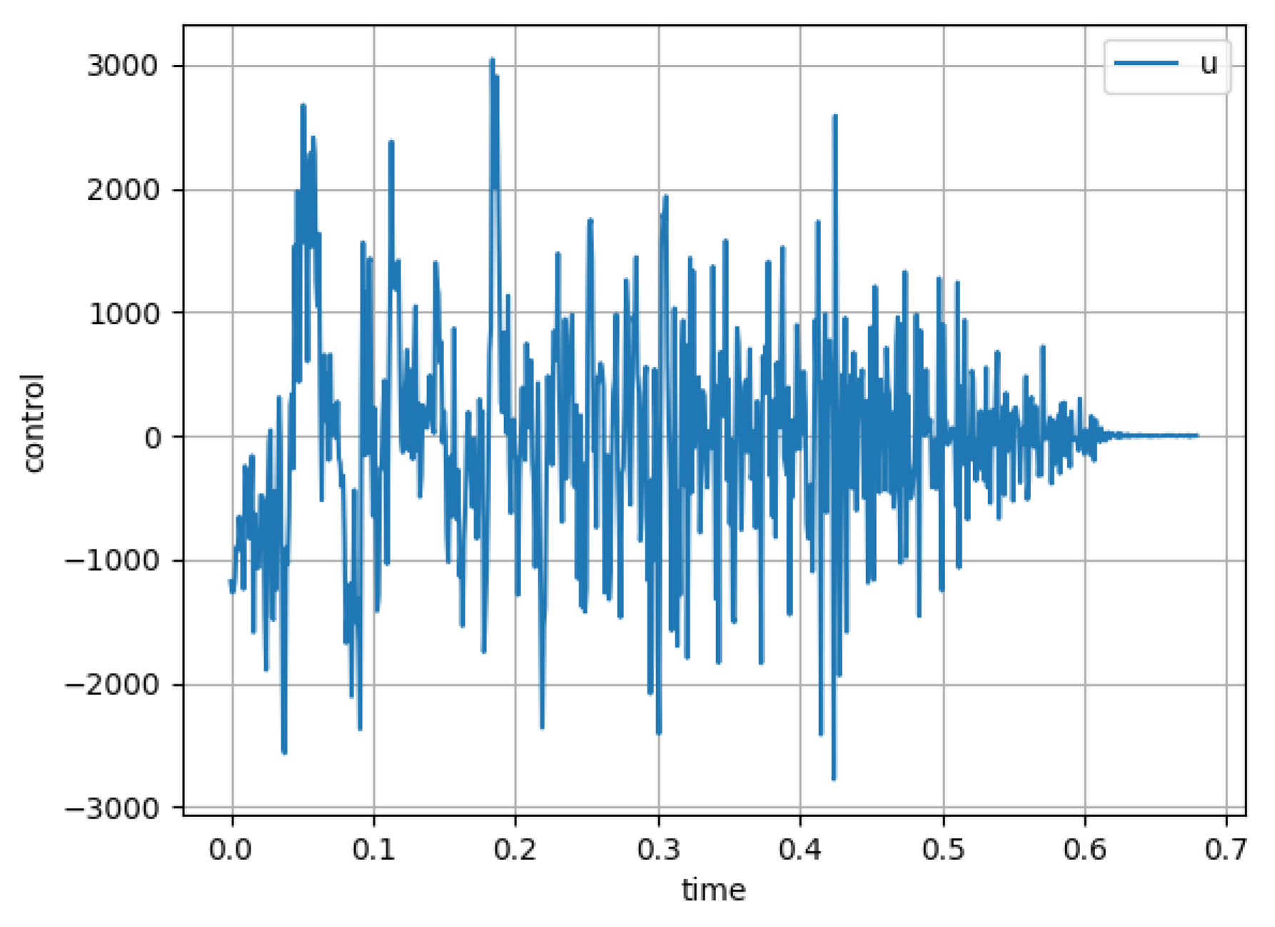
For simulation, we select randomly set the initial conditions as , and the parameters Figure 2a shows the state of system (44) without control u applied. Figure 2b shows the response of system (44) and (50). Figure 3 illustrates the effectiveness of controller u. According to Figure 4, we find that , which means that the prescribed-time mean-square stabilization is achieved. Therefore, the effectiveness of the controller design developed in Section 3 is demonstrated.
In the next example, we choose a nonlinear system to verify the effectiveness of the method in this paper.
Example 2.
Consider the following systems:
The derivation of this example will not be repeated. For simulation, we select , , and randomly set the initial conditions as , . Figure 5a shows the state of system (51) without control u applied. Figure 5b shows the response of system (51) with controller u for Example 2. Figure 6 illustrates the effectiveness of controller u. Therefore, the validity of the controller design developed in Section 3 is demonstrated.
5. Conclusions
In this paper, we discussed the specified time mean square stability problem of a class of leader-type stochastic nonlinear system (3) with the help of a new controller. Firstly, we defined new Lyapunov functions (11) and (17) for system (3). By developing a scale-free backstepping design method, a new controller has been designed to ensure that the equilibrium of the system origin is the time mean square stability specified in Theorem 1. At the same time, two important estimates, (32) and (33), were given. In addition, the special cases of circuit systems (43) and nonlinear systems (51) achieved the specified time mean square stability through the application of controllers. In future work, it is necessary to consider the influence of the time-delay of leader-type stochastic nonlinear systems.
Funding
This research received no external funding.
Data Availability Statement
Data availability is not applicable to this article as no new data were created or analyzed in this study.
Acknowledgments
The author really appreciates the valuable comments of the editors and reviewers.
Conflicts of Interest
The author declares no conflict of interest.
References
- Paternoster, B.; Shaikhet, L. About stability of nonlinear stochastic difference equations. Appl. Math. Lett. 2000, 13, 27–38. [Google Scholar] [CrossRef]
- Mao, X.R.; Yuan, C.G. Stochastic Differential Equations with Markovian Switching; Imperial College Press: London, UK, 2006. [Google Scholar]
- Verriest, E.I.; Michiels, W. Stability analysis of systems with stochastically varying delays. Syst. Control Lett. 2009, 58, 783–791. [Google Scholar] [CrossRef]
- Rafail, K. Stochastic Modelling and Applied Probability; Springer: Berlin/Heidelberg, Germany, 2012. [Google Scholar]
- Li, W.Q.; Krstic, M. Stochastic nonlinear prescribed-time stabilization and inverse optimality. IEEE Trans. Autom. Control 2012, 67, 1179–1193. [Google Scholar] [CrossRef]
- Elbsat, M.N.; Yaz, E.E. Robust and resilient finite-time control of a class of continuous-time nonlinear systems. IFAC Proc. Vol. 2012, 45, 15–20. [Google Scholar] [CrossRef]
- Lv, X.X.; Li, X.D. Finite time stability and controller design for nonlinear impulsive sampled-data systems with applications. ISA Trans. 2017, 70, 30–36. [Google Scholar] [CrossRef]
- Song, Y.D.; Wang, Y.J.; Holloway, J.; Krstic, M. Time-varying feedback for regulation of normal-form nonlinear systems in prescribed finite time. Automatica 2017, 82, 243–251. [Google Scholar] [CrossRef]
- Yaghobipour, S.; Yarahmadi, M. Optimal control design for a class of quantum stochastic systems with financial applications. Phys. A Stat. Mech. Its Appl. 2018, 512, 507–522. [Google Scholar] [CrossRef]
- Hansen, S.D.; Huang, W.Y.; Young, K.L.; Groves, J.T. Stochastic fluctuation sensing in a bistable phosphatidylinositol-based reaction diffusion system. Biophys. J. 2016, 110, 421a. [Google Scholar] [CrossRef]
- Polimeni, S.; Meraldi, L.; Moretti, L.; Leva, S.; Manzolini, G. Development and experimental validation of hierarchical energy management system based on stochastic model predictive control for off-grid microgrids. Adv. Appl. Energy 2021, 2, 100028. [Google Scholar] [CrossRef]
- Kumar, S.; Sharma, R.K.; Kamal, S. Design of Guidance Law with Predefined Upper Bound of Settling Time. IFAC-PapersOnLine 2022, 55, 418–423. [Google Scholar] [CrossRef]
- Kumar, S.; Soni, S.K.; Pal, A.K.; Kamal, S.; Xiong, X.G. Nonlinear Polytopic Systems with Predefined Time Convergence. IEEE Trans. Circuits Syst. II Express Briefs 2021. [CrossRef]
- Zhou, Y.; Wan, X.X.; Huang, C.X.; S, X. Yang. Finite-time stochastic synchronization of dynamic networks with nonlinear coupling strength via quantized intermittent control. Appl. Math. Comput. 2020, 376, 125157. [Google Scholar]
- Sun, K.L.; Yu, H.; Xia, X.H. Distributed control of nonlinear stochastic multi-agent systems with external disturbance and time-delay via event-triggered strategy. Neurocomputing 2021, 452, 275–283. [Google Scholar] [CrossRef]
- Wang, F.; Liu, Z.; Zhang, Y.; Chen, C.L.P. Adaptive finite-time control of stochastic nonlinear systems with actuator failures. Fuzzy Sets Syst. 2019, 374, 170–183. [Google Scholar] [CrossRef]
- Nacif, L.A.; Bessa, M.R. Stochastic nonlinear model with individualized plants and demand elasticity for large-scale hydro-thermal power systems. Electr. Power Syst. Res. 2023, 220, 109283. [Google Scholar] [CrossRef]
- Tan, Z.L.; Liu, Y.; Sun, J.Y.; Zhang, H.G.; Xie, X.P. Chaos synchronization control for stochastic nonlinear systems of interior pmsms based on fixed-time stability theorem. Appl. Math. Comput. 2022, 430, 127115. [Google Scholar] [CrossRef]
- Chen, W.S.; Jiao, L.C. Finite-time stability theorem of stochastic nonlinear systems. Automatica 2010, 46, 2105–2108. [Google Scholar] [CrossRef]
- Yin, J.L.; Khoo, S.Y.; Man, Z.H.; Yu, X.H. Finite-time stability and instability of stochastic nonlinear systems. Automatica 2011, 47, 2671–2677. [Google Scholar] [CrossRef]
- Arbi, A.; Cao, J.D.; Alsaedi, A. Improved synchronization analysis of competitive neural networks with time-varying delays. Nonlinear Anal. Model. Control 2018, 23, 82–107. [Google Scholar] [CrossRef]
- Ai, Z.D.; Zong, G.D. Finite-time stochastic input-to-state stability of impulsive switched stochastic nonlinear systems. Appl. Math. Comput. 2014, 245, 462–473. [Google Scholar]
- Li, W.Q.; Krstic, M. Prescribed-time mean-square nonlinear stochastic stabilization. IFACPapersOnLine 2020, 53, 2195–2200. [Google Scholar] [CrossRef]
- Li, W.Q.; Krstic, M. Prescribed-time output-feedback control of stochastic nonlinear systems. IEEE Trans. Autom. Control 2023, 68, 1431–1446. [Google Scholar] [CrossRef]
- Steeves, D.; Krstic, M.; Vazquez, R. Prescribed-time estimation and output regulation of the linearized schrodinger equation by backstepping. Eur. J. Control 2020, 55, 3–13. [Google Scholar] [CrossRef]
Figure 1.
Circuit system.
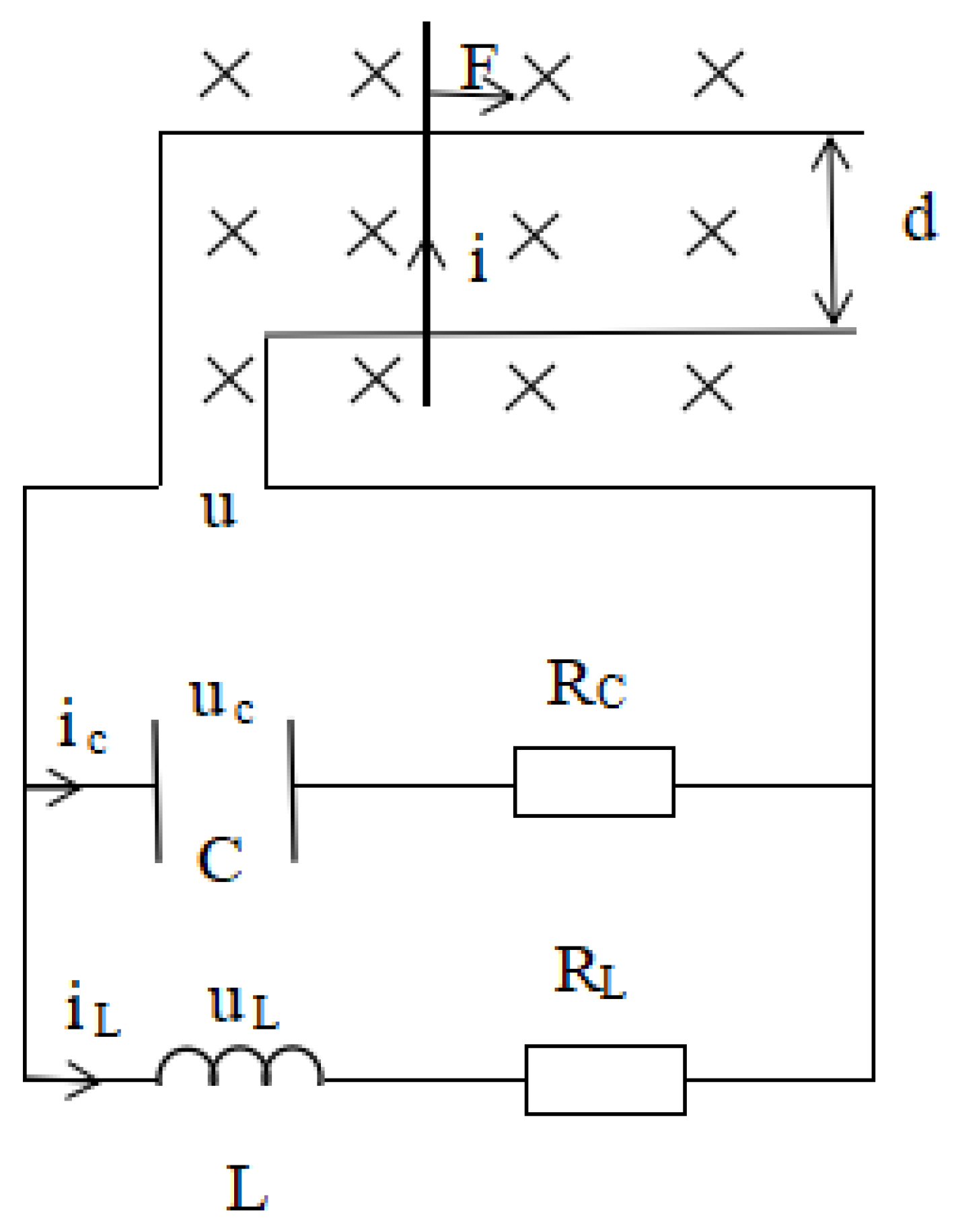
Figure 2.
Comparison of no control applied and control applied for Example 1.
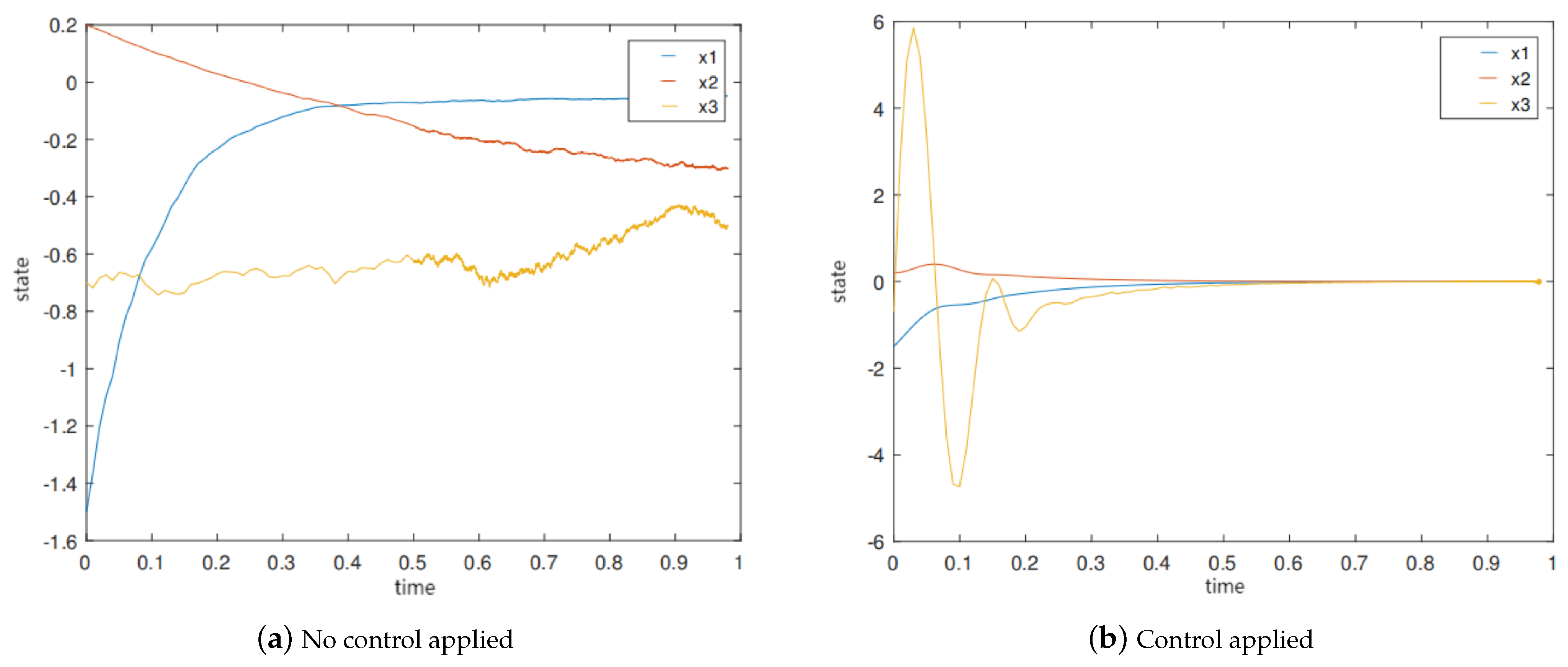
Figure 3.
Effectiveness of controller for Example 1.

Figure 4.
Stability analysis for Example 1.
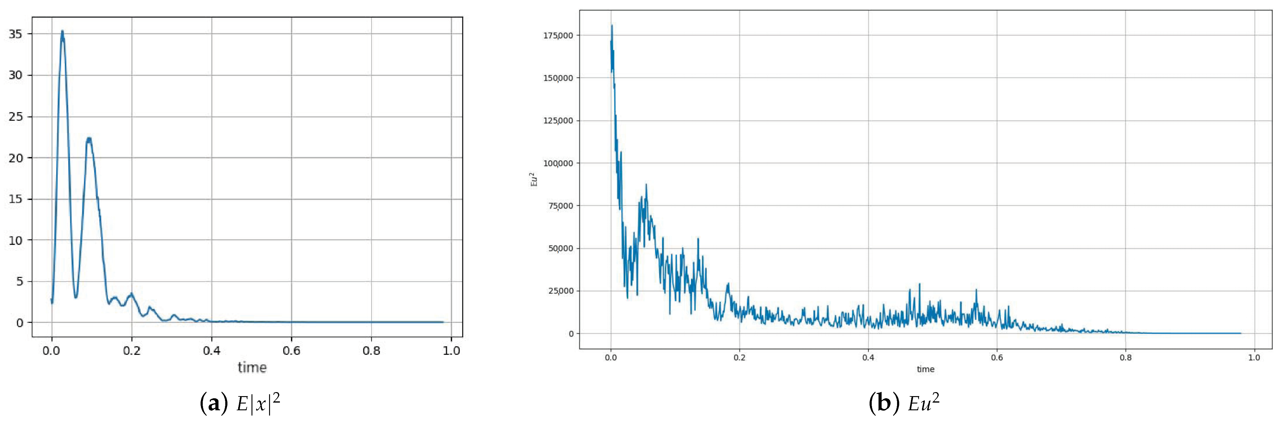
Figure 5.
Comparison of no control applied and control applied for Example 2.
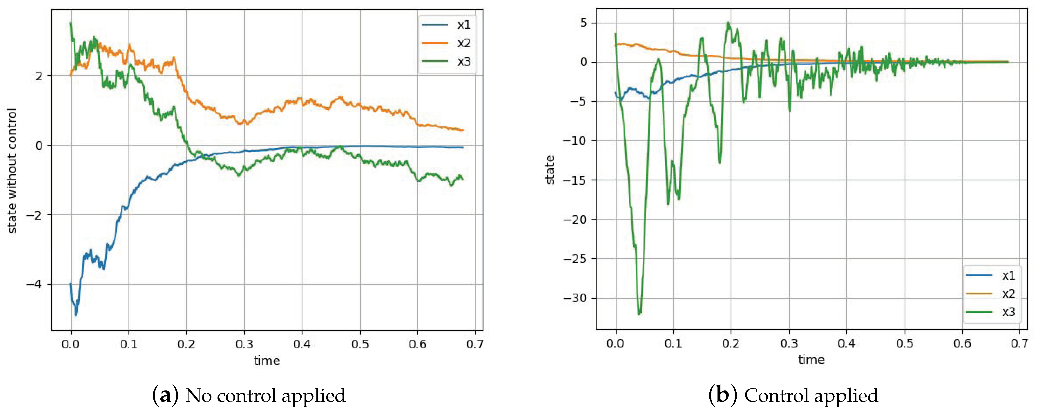
Figure 6.
Effectiveness of controller for Example 2.
Disclaimer/Publisher’s Note: The statements, opinions and data contained in all publications are solely those of the individual author(s) and contributor(s) and not of MDPI and/or the editor(s). MDPI and/or the editor(s) disclaim responsibility for any injury to people or property resulting from any ideas, methods, instructions or products referred to in the content. |
© 2023 by the author. Licensee MDPI, Basel, Switzerland. This article is an open access article distributed under the terms and conditions of the Creative Commons Attribution (CC BY) license (https://creativecommons.org/licenses/by/4.0/).
Share and Cite
MDPI and ACS Style
Zhang, H. Controller Design and Stability Analysis for a Class of Leader-Type Stochastic Nonlinear Systems. Symmetry 2023, 15, 2049. https://doi.org/10.3390/sym15112049
AMA Style
Zhang H. Controller Design and Stability Analysis for a Class of Leader-Type Stochastic Nonlinear Systems. Symmetry. 2023; 15(11):2049. https://doi.org/10.3390/sym15112049
Chicago/Turabian StyleZhang, Haiying. 2023. "Controller Design and Stability Analysis for a Class of Leader-Type Stochastic Nonlinear Systems" Symmetry 15, no. 11: 2049. https://doi.org/10.3390/sym15112049
Note that from the first issue of 2016, this journal uses article numbers instead of page numbers. See further details here.