A Preconditioner for Galerkin–Legendre Spectral All-at-Once System from Time-Space Fractional Diffusion Equation

Abstract

As a model that possesses both the potentialities of Caputo time fractional diffusion equation (Caputo-TFDE) and symmetric two-sided space fractional diffusion equation (Riesz-SFDE), time-space fractional diffusion equation (TSFDE) is widely applied in scientific and engineering fields to model anomalous diffusion phenomena including subdiffusion and superdiffusion. Due to the fact that fractional operators act on both temporal and spatial derivative terms in TSFDE, efficient solving for TSFDE is important, where the key is solving the corresponding discrete system efficiently. In this paper, we derive a Galerkin–Legendre spectral all-at-once system from the TSFDE, and then we develop a preconditioner to solve this system. Symmetry property of the coefficient matrix in this all-at-once system is destroyed so that the deduced all-at-once system is more convenient for parallel computing than the traditional timing-step scheme, and the proposed preconditioner can efficiently solve the corresponding all-at-once system from TSFDE with nonsmooth solution. Moreover, some relevant theoretical analyses are provided, and several numerical results are presented to show competitiveness of the proposed method.

1. Introduction

Classical integer order diffusion equation (IDE) is usually applied to describe normal diffusion phenomena such as the diffusion of particles in liquids or gases [1]. However, with further exploration for complicated diffusion phenomena in mechanics and engineering fields [2,3], researchers have encountered challenges in accurately utilizing IDE to simulate the diffusion motion of particles in fractal media (known as anomalous diffusion) [4]. Therefore, studies about time-space fractional diffusion equation (TSFDE) of the following form [5] are particularly popular

$$\begin{array}{c}\left\{\begin{array}{c}{}_0^c{D}_t^{\beta }u(x,t)=\kappa \frac{{\partial }^{\alpha }u(x,t)}{\partial {|x|}^{\alpha }}+g(x,t),(x,t)\in (a,b)\times (0,T],\hfill \\ u(x,0)=\psi (x),x\in (a,b),\hfill \\ u(a,t)=u(b,t)=0,t\in (0,T],\hfill \end{array}\right.\hfill \end{array}$$

(1)

where $\kappa >0$ is the generalized diffusion coefficient, $u(x,t)$ exhibits the concentration of interest at location x of time t, $g(x,t)$ represents the source item and is a continuous function, ${\psi }_{(x)}$ is a given smooth function, $(a,b)$ and $(0,T]$ represent spatial and temporal domains, ${}_0^c{D}_t^{\beta }u(x,t)$ and $\frac{{\partial }^{\alpha }u(x,t)}{\partial {|x|}^{\alpha }}$ are the Caputo fractional derivatives and the Riesz fractional derivatives defined as

$$\begin{array}{c}{}_0^c{D}_t^{\beta }u(x,t)=\frac{1}{\Gamma (1-\beta )}{\int }_0^t{(t-\theta )}^{-\beta }\frac{\partial u(x,\theta )}{\partial \theta }d\theta ,\hfill \\ \frac{{\partial }^{\alpha }u(x,t)}{\partial {|x|}^{\alpha }}=\frac{1}{2cos(\alpha \pi /2)}\frac{{\partial }^2}{\partial x^2}{\int }_{-\infty }^{+\infty }{|x-\eta |}^{1-\alpha }u(\eta ,t)d\eta ,\hfill \end{array}$$

where $\Gamma (·)$ is the Gamma function, and $\beta \in (0,1)$ and $\alpha \in (1,2)$ are fractional orders of the time and space derivatives, respectively.

For $\beta =1,\alpha \in (1,2)$, Equation (1) is equivalent to a symmetric case of the two-sided fractional diffusion equation, which is called Riesz-space fractional diffusion equation (Riesz-SFDE) [6]. Riesz fractional operator is an effective tool to explore nonlocal effects for engineering and physics applications [7], hence Riesz-SFDE is usually applied to model complicated phenomenon with path dependency and nonlocality [8]. Equation (1) is reduced to Caputo-time fractional diffusion equation (Caputo-TFDE) if $\beta \in (0,1),\alpha =2$. Note that Caputo derivative is defined pointwise for continuously differentiable functions [9], so that Caputo fractional differential operator can well overcome the supersingularity [10], and then Caputo-TFDE is practical for modeling long term memory phenomenon [11]. As a model that possesses both potentialities of Caputo-TFDE and symmetric two-sided space fractional diffusion equation (Riesz-SFDE) [12], Equation (1) is usually used to describe subdiffusion phenomenon if $0<2\beta /\alpha <1$, superdiffusion phenomenon if $2\beta /\alpha >1$, and normal diffusion if $\alpha =2\beta$. In fact, for simulating the anomalous diffusion of particles, coefficients of fractional derivative in Equation (1) are usually used to describe the competitive relationship between long waiting time and large jumps of particles [13]. Moreover, Equation (1) is usually related to the scaling limits of the continuous time random walks and extensively applied in numerous engineering and scientific fields [14]. For instance, in ocean dynamics, Equation (1) can be used to describe the anomalous transport problem that the sticky trajectories within the boundary layers of the islands, where the boundary layers of the islands is regarded as a fractal support [15], and in financial economics, by modeling prices as random variables and varying waiting times between two consecutive transactions into a stochastic fashion. The authors in Ref. [16] utilize Equation (1) to model the behavior of returns and derive a rather general phenomenological theory in financial markets. In addition, as a foundation for more complicated diffusion modeling, Equation (1) can also be developed into variable-order model [17], distributed-order model [18], random-order model [19], nonlinear model [20], and other forms [21] for better application.

Due to the nonlocality of the fractional derivatives, analytical solutions for Equation (1) are usually difficult to obtain explicitly. Accordingly, numerical schemes for their approximate solutions have received much attention [22]. As a numerical scheme that typically converges with high order [23], in recent years, spectral methods are well developed for discretizing those FDEs. For example, after applying the generalized Jacobi functions and Fourier-like basis functions on time and space of TFDE respectively, Sheng and Shen [24] obtained a space-time Petrov-Galerkin spectral method for TFDE, this method can reach spectral accuracy in both space and time. To further improve the efficiency in discretization, Li and Xu [25] proposed a new spectral method for TFDE. This method can solve the problem with long-time solution since the “global time dependence” makes the storage requirement considerably relaxed. However, Li and Xu only applied this method to a 1D problem, for the discretization of high-order TFDE, by utilizing Legendre polynomials and their variants to approximate both temporal and spatial variables. Fakhar-Izadi and Shabgard [26] derived a new time-space spectral Galerkin method. This method can be stable for a kind of fourth-order TFDE. In fact, for the inverse problem of TFDE, spectral methods can also reach an exponential convergence. Based on the work of Lin et al. [27], who applied the spectral scheme to approximate TFDE, Ye et al. [28] proposed a spectral optimization method for its inverse problem, under the assumption that the optimal initial condition is smooth. The proposed method can indeed reach the exponential convergence rate. In addition, to further exploit the stability and high convergence of spectral methods in solving different variants of Equation (1), Zaky et al. [29,30] developed a class of semi-implicit Galerkin–Legendre spectral schemes. These methods are stable for nonlinear time-space fractional Schrödinger equation and can reach spectral accuracy even for those TSFDEs with nonsmooth solutions. Discussions about spectral methods for solving other variants of Equation (1) are exploited in Refs. [31,32,33,34,35]. The methods in these works are stable and can usually reach spectral accuracy. Moreover, in order to further save the computational cost of those methods, numerous fast algorithms are also designed for solving TFDE [36], TSFDE [37], and their variants [38,39,40]. In these methods, by utilizing the sum-of-exponential technique to approximate the kernel function in the tempered Caputo fractional derivative or using the Laplace transform for time integration of a semi-discretized system, these methods are stable and usually have a low computational cost.

One may observe that with the timing-step schemes mentioned above, one should solve the discrete system on each time level sequentially since the right-hand-side vector usually depends on the solution from a previous time level, which may lead to less convenience for parallel computing in the solving of Equation (1). For this reason, people turn to studying the all-at-once technique. At first, the all-at-once technique was proposed for solving the evolutionary equation with integer order. In these works, McDonald [41], Goddard [42], Lin [43], and Wu [44] stacked all the time steps in a vector to obtain an all-at-once system in the discretization process and then solved it. The right-hand-side vectors in these corresponding all-at-once systems only rely on the solutions at the initial time, and this phenomenon is truly convenient for parallel computing. After that, with the exploration of efficient solving for Equation (1), the all-at-once technique combined with finite differential method (FDM) or finite element method (FEM) spatial discretization and uniform temporal discretization (such as L1 [45], L1-2 [46], and $L2$-$1_{\sigma }$ [47]) has been well utilized to solve those fractional diffusion equation, and the solving of corresponding all-at-once systems are also well studied. In general, coefficient matrices in these all-at-once systems from the above scheme no longer maintain the symmetry property but turn into Toeplitz block lower triangular matrices with Toeplitz subblocks. In order to reduce the computational complexity in the solving of those kinds of all-at-once systems, Huang, et al. [48] and Jia, et al. [49] proposed two fast methods. These two methods are mainly based on the divide and conquer technique, and they are well applied to Equation (1) and TFDE with space-time-dependent variable order, respectively.

Note that the coefficient matrix in the above all-at-once system is usually ill-conditioned, so utilization of a preconditioners is necessary [50]. Block preconditioner is a straightforward method to improve the illness of the coefficient matrix [51]. Based on this idea, Chen et al. [52] proposed four block preconditioners for solving the all-at-once system originating from Equation (1). Among these four block preconditioners, the banded block triangular preconditioner usually outperforms the other three if $\beta$ is close to one. Besides, Zhao [53], Gu [54,55], and Zhu [56] conducted extensive research on block preconditioning strategies for solving the all-at-once system especially those with Toeplitz coefficient matrix. These block preconditioners proposed by them can effectively accelerate the matrix-vector product and can usually reach the linear computing complexity. Furthermore, for the Volterra subdiffusion problem discrete by FDM in space and with combination of graded and uniform time-steps temporal discretization, Zhao et al. [57] combined a block lower tridiagonal preconditioner and a semi-circulant preconditioner to solve the corresponding all-at-once system. This method can also be extended to solve the system arising from semilinear subdiffusion problems.

Based on the above observations, we note that solving Equation (1) using spectral methods typically yields high-order discretization accuracy. However, traditional timing-step schemes are not convenient for parallel computing, and there is limited research on combining spectral methods with the graded $L1$ scheme and the all-at-once technique to solve Equation (1). Besides, the coefficient matrix of the all-at-once system obtained by spectral-method spatial discretization and graded $L1$ temporal discretization in Equation (1) no longer maintains the Toeplitz structure, and the preconditioners mentioned above are not appropriate for solving the corresponding Galerkin–Legendre spectral all-at-once system. Therefore, in order to improve the efficiency of solving Equation (1), in this paper, we mainly focus on deriving and solving the corresponding Galerkin–Legendre spectral all-at-once system that arises from Equation (1). The main contribution of the present paper has two aspects: (i). This is the first study to combine the all-at-once technique with the Galerkin–Legendre spectral method and graded $L1$ method to solve time-space fractional diffusion Equation (1), which is more convenient for parallel computing than the traditional timing-step spectral scheme. (ii). A new preconditioner is proposed to improve the efficiency of solving the corresponding Galerkin–Legendre spectral all-at-once system arising from Equation (1), and relevant theoretical analyses and numerical experiments are also provided to show the effectiveness of the proposed method.

The remaining part of this paper is organized as follows. In the following section, the graded $L1$-Galerkin–Legendre spectral scheme (G$L1$-GLS) is derived to approximate Equation (1) and then a Galerkin–Legendre spectral all-at-once system is obtained. In Section 3, based on the sparse pattern of the coefficient matrix, a block L-diagonal preconditioner is proposed to accelerate solving the all-at-once system and some relevant theoretical analyses are also provided. Numerical results are given in Section 4 to show the efficiency of the general block L-diagonal preconditioner, and selection of parameter in the proposed preconditioner is also discussed experimentally. Finally, concluding remarks are presented in Section 5.

2. GL1-GLS Discretization and the All-at-Once System

In this section, the graded $L1$-Galerkin–Legendre spectral (G$L1$-GLS) scheme [29] is applied to approximate Equation (1). Then, with several auxiliary symbols, a Galerkin–Legendre spectral all-at-once system is obtained.

2.1. The Time-Stepping Discretization

Notice that the solutions of Equation (1) may be non-smooth and singular near $t=0$ even though the initial conditions and source terms are smooth, and the graded $L1$ scheme can handle this problem well. Thus, in the following, the graded $L1$ scheme is utilized for the temporal discretization of Equation (1).

Lemma 1

([29]). For a positive integer M and $i=1,2,\cdots ,M$, let ${\{t_i=T{(i/M)}^{\gamma }\}}_{i=0}^M$ be the graded mesh with grading parameter $\gamma \ge 1$, and denote the temporal step-size ${\tau }_i$ of time $t_i$ by ${\tau }_i\equiv t_i-t_{i-1}$. Let ${\left\{u^n\right\}}_{n=0}^M$ be a sequence of functions defined on $[a,b]$. Then the graded discrete time-fractional difference Caputo operator ${\Delta }_M^{\beta }{u}^n$ is given by

$${\Delta }_M^{\beta }{u}^n={\Sigma }_{i=1}^n{\tilde{a}}_{n-i}^n{\delta }_t{u}^i={\Sigma }_{i=0}^n{\tilde{b}}_{n-i}^n{u}^i,$$

(2)

where

$$\begin{array}{c}{\tilde{a}}_{n-i}^n=\frac{1}{\Gamma (2-\beta )}\frac{{(t_n-t_{i-1})}^{1-\beta }-{(t_n-t_i)}^{1-\beta }}{t_i-t_{i-1}},1\le i\le n,\hfill \\ {\tilde{b}}_0^n={\tilde{a}}_0^n,{\tilde{b}}_n^n=-{\tilde{a}}_{n-1}^n,{\tilde{b}}_{n-i}^n={\tilde{a}}_{n-i}^n-{\tilde{a}}_{n-i-1}^n<0,\forall i=1,2,\cdots ,n-1.\hfill \end{array}$$

Since the spectral methods are usually with high-order discretization accuracy, in the following, the Galerkin–Legendre spectral scheme in [29] is used for the spatial discretization of Equation (1).

Lemma 2

([29]). Given a function space ${\mathcal{W}}_N^0\equiv span\{{\phi }_n(x):n=0,1,\cdots ,N-2\}$. Then for each $\widehat{x}\in [-1,1]$, the base function ${\phi }_n$ of spectral methods can be given by

$$\begin{array}{c}{\phi }_n(x)=L_n(\widehat{x})-L_{n+2}(\widehat{x})=\frac{2n+3}{2(n+1)}(1-{\widehat{x}}^2)J_n^{1,1}(\widehat{x}),\hfill \end{array}$$

(3)

where $x=\frac{1}{2}((b-a)\widehat{x}+a+b)\in [a,b]$ and for $\mu ,\nu >-1$, $J_i^{\mu ,\nu }(x)$ is the i-$th$ order Jacobi polynomial of index defined on $[-1,1]$.

Let $u_N^n$ be the discrete approximation of solution $u(x,t_n)\in {\mathcal{W}}_N$ for $x\in [a,b]$ and $0\le i\le n$. Then, we take Equations (2) and (3) into Equation (1), and get the following G$L1$-GLS scheme for Equation (1).

$$\begin{array}{c}\left\{\begin{array}{c}{\tilde{a}}_0^n(u_N^n,v)-\kappa (\frac{{\partial }^{\alpha }}{\partial {|x|}^{\alpha }}{u}_N^n,v)={\tilde{a}}_{n-1}^n(u_N^0,v)-{\Sigma }_{i=1}^{n-1}{\tilde{b}}_{n-i}^n(u_N^i,v)+(I_N{g}^n,v),\hfill \\ u_N^0=P_N\psi ,\forall v\in {\mathcal{W}}_N^0,\forall n=1,2,\cdots ,M,\hfill \end{array}\right.\hfill \end{array}$$

where $P_N$ is an appropriate projection operator [29]. Denote

$$\begin{array}{c}{S}_{i,j}={\int }_{\Omega }{}_a{D}_x^{\frac{\alpha }{2}}{\phi }_i{(x)}_x{D}_b^{\frac{\alpha }{2}}{\phi }_j(x)dx,S={(s_{i,j})}_{i,j=0}^{N-2},\hfill \\ m_{i,j}={\int }_{\Omega }{\phi }_i(x){\phi }_j(x)dx,\overline{M}={(m_{i,j})}_{i,j=0}^{N-2},\hfill \\ g_{i,n}={\int }_{\Omega }{\phi }_i(x)I_N{g}^{n}dx,F^n={(g_0^n,g_1^n,\cdots ,g_{N-2}^n,)}^T,\hfill \\ U^n={({\widehat{u}}_0^n,{\widehat{u}}_1^n,\cdots ,{\widehat{u}}_0^{N-2})}^T.\hfill \end{array}$$

Then the G$L1$-GLS scheme can be rewritten into the matrix-vector form as

$$\begin{array}{c}({\tilde{a}}_0^n\overline{M}-\kappa c_{\alpha }(S+S^T))U^n=-{\Sigma }_{j=0}^{n-1}{\tilde{b}}_{n-j}^n\overline{M}{U}^j+F^n,n=1,2,\cdots ,M,\hfill \end{array}$$

(4)

where $c_{\alpha }=-\frac{1}{2}sec(\frac{\pi \alpha }{2})$.

According to Ref. [29], under certain assumptions about the regularity of the unique solution for Equation (1), the numerical solution obtained from above G$L1$-GLS scheme can achieve an optimal time convergence order for the optimal grading parameter ${\gamma }_{opt}=max\left\{1,(2-\beta )/\sigma \right\}$, where $\sigma =[0,1]\cup [1,2]$ is used to reflect the regularity of the solution. Furthermore, more detailed convergence analyses of above G$L1$-GLS scheme can be found in Ref. [29].

From Equation (4), we find that based on the above G$L1$-GLS scheme, one needs to solve the discrete system on each time level sequentially since the right-hand-side vector in Equation (4) usually depends on the solution on a previous time level and this may lead to less convenience for parallel computing in the solving of Equation (1). For this reason, in the next subsection, the all-at-once technique is considered, and then Equation (4) can be transformed into the Galerkin–Legendre spectral all-at-once system, which is more convenient for parallel computing.

2.2. The Galerkin–Legendre Spectral All-at-Once System

To simplify the derivation of the Galerkin–Legendre spectral all-at-once system, several auxiliary symbols are introduced: O and I are zero and identity matrices of suitable orders. Furthermore, denote

$$\begin{array}{c}{A}_0^n={\tilde{a}}_0^n\overline{M}-\kappa c_{\alpha }(S+S^T),1\le n\le M,\hfill \\ A_k^n={\tilde{b}}_k^n\overline{M},1\le k\le M-1,\hfill \\ b^n=-{\tilde{b}}_k^n\overline{M}{U}^0+F^n.\hfill \end{array}$$

Then, based on Equation (4), we can get the following Galerkin–Legendre spectral all-at-once system

$$\mathcal{A}u=b,$$

(5)

where $u={[{(U^1)}^T,{(U^2)}^T,\cdots ,{(U^M)}^T]}^T$, $b={[{(b^1)}^T,\cdots ,{(b^M)}^T]}^T$ and

$$\mathcal{A}=\left(\begin{array}{cccccc}{A}_0^1& O& O& \cdots & O& O\\ A_1^2& A_0^2& O& O& ⋮& ⋮\\ ⋮& \ddots & \ddots & \ddots & ⋮& ⋮\\ A_{l-1}^l& \ddots & \ddots & \ddots & O& O\\ ⋮& \ddots & \ddots & \ddots & ⋮& ⋮\\ A_{N-1}^{M-1}& \cdots & A_{l-1}^M& \cdots & A_1^M& A_0^M\end{array}\right).$$

(6)

Note that the right-hand-side vector in Equation (5) only depends on the solution in the initial time level, and this makes Equation (5) truly convenient for parallel computing. In addition, from Equation (6), we find that although the block lower triangular coefficient matrix $\mathcal{A}$ in Equation (5) no longer maintains the symmetry property directly like $A_0^n$ in Equation (4), each subblock of $\mathcal{A}$ is symmetric. In addition, by “⊗”, we denote the Kronecker product. Then the coefficient matrix in Equation (5) can be written as $\mathcal{A}=B\otimes \overline{M}-I_M\otimes (\kappa c_{\alpha }(S+S^T))$, where

$$B=\left(\begin{array}{cccccc}{\tilde{a}}_0^1& 0& 0& \cdots & 0& 0\\ {\tilde{b}}_1^2& {\tilde{a}}_0^2& 0& 0& \cdots & 0\\ {\tilde{b}}_2^3& {\tilde{b}}_1^3& {\tilde{a}}_0^3& \ddots & \ddots & 0\\ ⋮& \ddots & \ddots & \ddots & \ddots & ⋮\\ {\tilde{b}}_{M-2}^{M-1}& \ddots & \ddots & \ddots & {\tilde{a}}_0^{M-1}& 0\\ {\tilde{b}}_{M-1}^M& {\tilde{b}}_{M-2}^M& \cdots & {\tilde{b}}_2^M& {\tilde{b}}_1^M& {\tilde{a}}_0^M\end{array}\right).$$

(7)

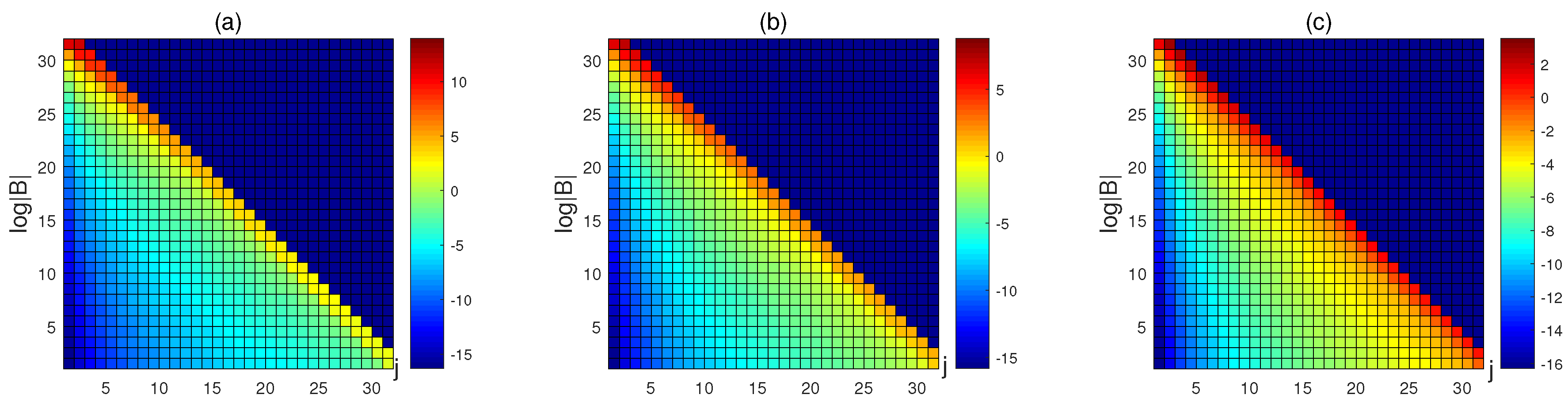
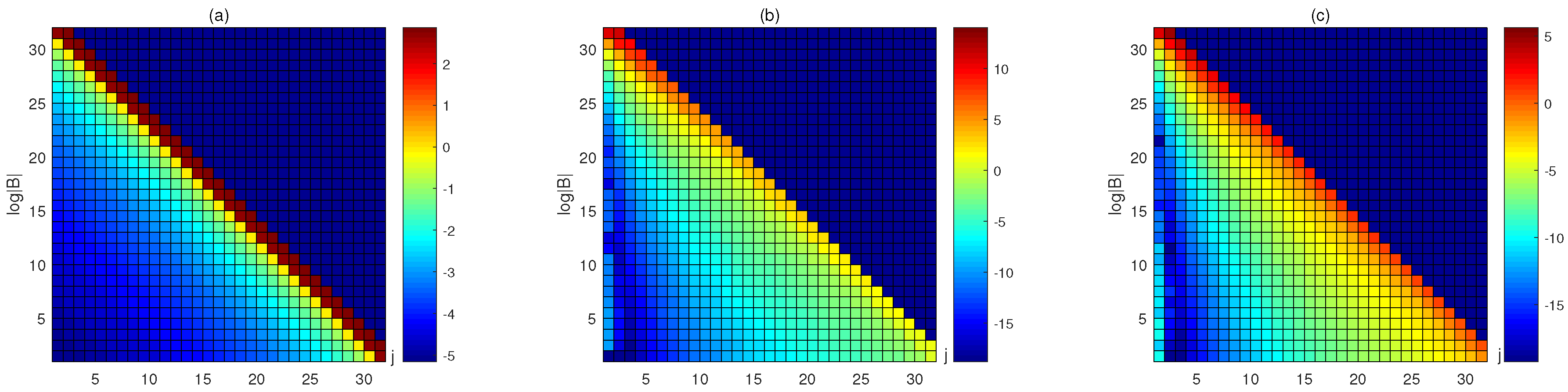
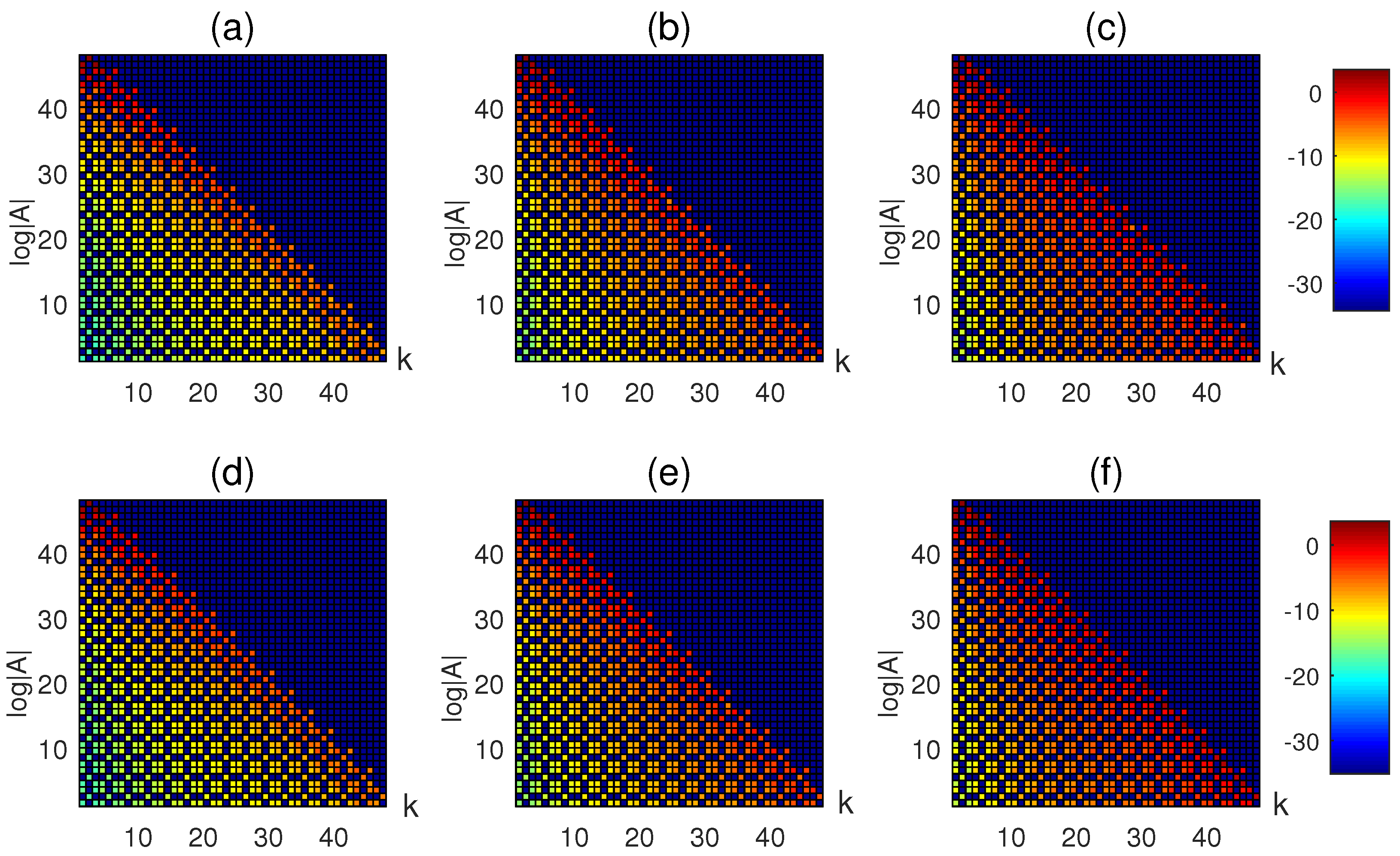
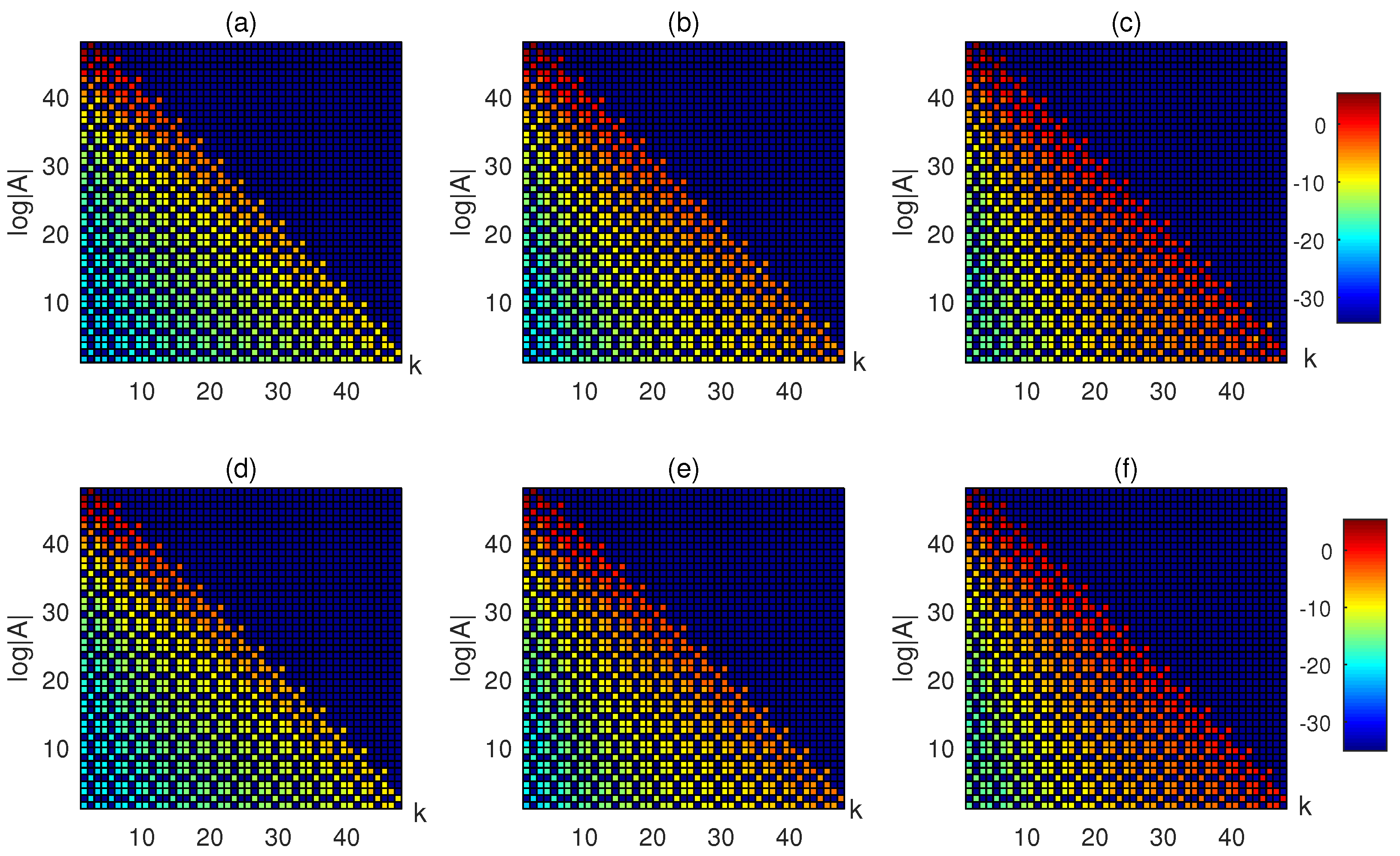
From Equation (7) and Lemma 1, we find that values of elements in matrix B are mainly affected by the grading parameter $\gamma$ of temporal graded mesh and the fractional order $\beta$ of time derivative. Since $\mathcal{A}=B\otimes \overline{M}-I_M\otimes (\kappa c_{\alpha }(S+S^T))$, $\gamma$ and $\beta$ may also affect values of elements in matrix $\mathcal{A}$. Besides, values of elements in matrix $\mathcal{A}$ may also be affected by fractional order $\alpha$ of space derivative. Details about the elements of matrix B and $\mathcal{A}$ with variant parameters are shown in Figure 1, Figure 2, Figure 3 and Figure 4, respectively.

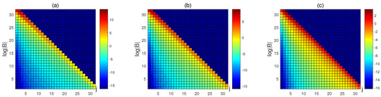
Figure 1. The elements of matrix B in $[0,T]=[0,1]$ with $M=32$, $\gamma =5$ and in (a–c), $\beta$ is taken as $0.8,0.5,0.2$, respectively.

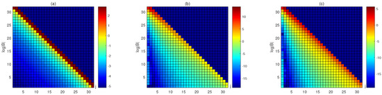
Figure 2. The elements of matrix B in $[0,T]=[0,1]$ with $M=32,\gamma =8$ and in (a–c), $\beta$ is taken as $0.8,0.5,0.2$, respectively.

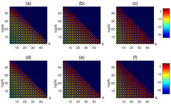
Figure 3. The elements of the coefficient matrix with $\gamma =5$, $M=16,N=4$, where (a–c) are those of $\mathcal{A}$ in $[a,b]\times [0,T]=[-1,1]\times [0,1]$, and $\alpha =1.2,\beta =0.8$, $\alpha =1.5,\beta =0.5$, $\alpha =1.8,\beta =0.2$, (d–f) are those of $\mathcal{A}$ in $[a,b]\times [0,T]=[0,2]\times [0,1]$, and $\alpha =1.2,\beta =0.8$, $\alpha =1.5,\beta =0.5$, $\alpha =1.8,\beta =0.2$, respectively.

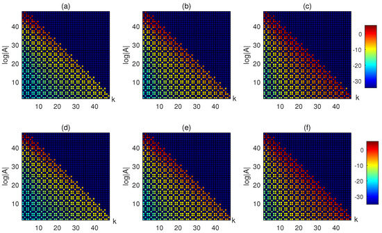
Figure 4. The elements of the coefficient matrix with $\gamma =8$, $M=16,N=4$, where (a–c) are those of $\mathcal{A}$ in $[a,b]\times [0,T]=[-1,1]\times [0,1]$, and $\alpha =1.2,\beta =0.8$, $\alpha =1.5,\beta =0.5$, $\alpha =1.8,\beta =0.2$, (d–f) are those of $\mathcal{A}$ in $[a,b]\times [0,T]=[0,2]\times [0,1]$, and $\alpha =1.2,\beta =0.8$, $\alpha =1.5,\beta =0.5$, $\alpha =1.8,\beta =0.2$, respectively.

To solve the linear system, Krylov subspace methods such as BICGSTAB and GMRES are usually efficient if the condition number of the coefficient matrix is small. Notice that the coefficient matrix $\mathcal{A}$ in Equation (5) is usually ill-conditioned. Therefore, an effective preconditioner, which can reduce the condition number or make the spectral distribution of the coefficient matrix cluster around 1 should be employed [50]. In the next section, we will mainly focus on developing such an efficient preconditioner.

3. The Block L-Diagonal Preconditioner

In this section, we propose a block L-diagonal preconditioner ${\mathcal{M}}_L$ to solve Equation (5) and some corresponding theoretical analyses will also be provided.

3.1. Derivation of the General Block L-Diagonal Preconditioner ${\mathcal{M}}_L$

Firstly, we focus on observing the sparsity pattern of matrix B and the coefficient matrix $\mathcal{A}=B\otimes \overline{M}-I_M\otimes (\kappa c_{\alpha }(S+S^T))$.

As is shown in Figure 1 and Figure 2, the diagonal entries of the coefficient matrix B are decreased. Since $\mathcal{A}=B\otimes \overline{M}-I_M\otimes (\kappa c_{\alpha }(S+S^T))$, as can be seen from Figure 3 and Figure 4, the main information of $\mathcal{A}$ is gathered in the first L-nonzero diagonal blocks, where L is usually larger than 3. Based on the above observation, we can naturally propose a block L-diagonal preconditioner ${\mathcal{M}}_L=B_L\otimes \overline{M}-I_M\otimes (\kappa c_{\alpha }(S+S^T))$ to solve Equation (5), where

$$B_L=\left(\begin{array}{cccccc}{\tilde{a}}_0^1& 0& 0& \cdots & 0& 0\\ {\tilde{b}}_1^2& {\tilde{a}}_0^2& 0& 0& \cdots & 0\\ ⋮& \ddots & \ddots & \ddots & ⋮& 0\\ {\tilde{b}}_{L-1}^l& \ddots & \ddots & \ddots & ⋮& 0\\ ⋮& \ddots & \ddots & \ddots & ⋮& 0\\ 0& \cdots & {\tilde{b}}_{L-1}^M& \cdots & {\tilde{b}}_1^M& {\tilde{a}}_0^M\end{array}\right).$$

It is obvious that ${\mathcal{M}}_1=blockdiag(\mathcal{A})$ if $L=1$.

3.2. Theoretical Analyses of the Block L-Diagonal Preconditioner

For convenience of discussing the nonsingularity of the L-diagonal preconditioner ${\mathcal{M}}_L$, we present the following two lemmas.

Lemma 3

([29]). The nonzero components in the mass matrix $\overline{M}$ in Equation (5) are

$$\begin{array}{c}{m}_{ij}=m_{ji}=\left\{\begin{array}{c}\frac{b-a}{2j+1}+\frac{b-a}{2j+5},\forall i=j,\hfill \\ -\frac{b-a}{2j+5},\forall i=j+2.\hfill \end{array}\right.\hfill \end{array}$$

Lemma 4

([29]). The components of the stiffness matrix S are $s_{ij}=a_i^j-a_i^{j+2}-a_{i+2}^j+a_{i+2}^{j+2}$, for each $i,j=0,1,\cdots ,N-2$, and

$$\begin{array}{cc}\hfill a_i^j& ={(\frac{b-a}{2})}^{1-\alpha }\frac{\Gamma (i+1)\Gamma (j+1)}{\Gamma (i-\frac{\alpha }{2}+1)\Gamma (j-\frac{\alpha }{2}+1)}\hfill \\ & ·\sum _{r=0}^N{\varpi }_r^{-\frac{\alpha }{2},-\frac{\alpha }{2}}{J}_i^{\frac{\alpha }{2},-\frac{\alpha }{2}}(x_r^{-\frac{\alpha }{2},-\frac{\alpha }{2}})J_j^{-\frac{\alpha }{2},\frac{\alpha }{2}}(x_r^{-\frac{\alpha }{2},-\frac{\alpha }{2}}),\hfill \end{array}$$

where $\Gamma (·)$ is the Gamma function, $J_i^{\mu ,\nu }(x)$ is the i-$th$ order Jacobi polynomial of index defined on $[-1,1]$, $\left\{x_r^{-\frac{\alpha }{2},-\frac{\alpha }{2}},{\varpi }_r^{-\frac{\alpha }{2},-\frac{\alpha }{2}}\right\}$ is the set of Jacobi–Gauss points and weights with respect to the weight function ${\omega }^{-\frac{\alpha }{2},-\frac{\alpha }{2}}$$={(1-x)}^{-\frac{\alpha }{2}}{(1+x)}^{-\frac{\alpha }{2}}$.

Lemma 3 clarifies that $\overline{M}$ is symmetric positive definite and Lemma 4 shows detailed components of matrix S. Notice that ${\tilde{a}}_0^n>0$, $c_{\alpha }>0$ and $\kappa$ is a positive constant. Then, from Lemmas 3 and 4, we can see that all main diagonal blocks $A_0^n={\tilde{a}}_0^n\overline{M}-\kappa c_{\alpha }(S+S^T),1\le n\le M$ of the coefficient matrix $\mathcal{A}$ in Equation (5) is symmetric and invertible. Thus the coefficient matrix $\mathcal{A}$ and the preconditioner ${\mathcal{M}}_L$ are nonsingular.

In order to analyze the approximation effect of block L-diagonal preconditioner ${\mathcal{M}}_L$ on $\mathcal{A}$, we present the estimation for the approximate error between ${\mathcal{M}}_L$ and $\mathcal{A}$ in the following theorem.

Theorem 1.

Let $|\frac{{\varsigma }_{j-1}-{\varsigma }_j}{{\tau }_j}-\frac{{\varsigma }_{j-2}-{\varsigma }_{j-1}}{{\tau }_{j-1}}|<c_j^n$, where ${\tau }_j=t_j-t_{j-1}$ and ${\varsigma }_j^n={(t_n-t_j)}^{1-\beta }$. Denote $\mathcal{E}=\mathcal{A}-{\mathcal{M}}_L$. Then we have

$$||\mathcal{E}||{}_{\infty }\le \frac{13(b-a)}{21·\Gamma (2-\beta )}·max\left\{\sum _{j=l-1}^{M-1}{c}_j^n,1\le n\le M\right\}.$$

Proof. 

Notice that

$$\begin{array}{c}\hfill \mathcal{A}=B\otimes \overline{M}+I_M\otimes (\kappa c_{\alpha }(S+S^T)),\\ \hfill {\mathcal{M}}_L=B_L\otimes \overline{M}+I_M\otimes (\kappa c_{\alpha }(S+S^T)).\end{array}$$

Then we have

$$\begin{array}{c}\mathcal{E}=\mathcal{A}-{\mathcal{M}}_L=(B-B_L)\otimes \overline{M}.\hfill \end{array}$$

From Lemma 3, we know that

$$\begin{array}{cc}\hfill ||\overline{M}{||}_{\infty }& =max\left\{\frac{b-a}{2i+1}+\frac{2(b-a)}{2i+5},1\le i\le N-1\right\}\hfill \\ & \le \frac{b-a}{3}+\frac{2(b-a)}{7}=\frac{13(b-a)}{21}.\hfill \end{array}$$

Denote $|\frac{{\varsigma }_{j-1}^n-{\varsigma }_j^n}{{\tau }_j}-\frac{{\varsigma }_{j-2}^n-{\varsigma }_{j-1}^n}{{\tau }_{j-1}}|<c_j^n$, where ${\tau }_j=t_j-t_{j-1}$ and ${\varsigma }_j^n={(t_n-t_j)}^{1-\beta }$. Thus we can get

$$\begin{array}{cc}\hfill ||\mathcal{E}||{}_{\infty }& =||(B-B_L)\otimes \overline{M}||{}_{\infty }\hfill \\ & =||(B-B_L)||{}_{\infty }·||\overline{M}||{}_{\infty }\hfill \\ & \le max\left\{\sum _{j=l-1}^{M-1}|b_j^n||\overline{M}{||}_{\infty },1\le n\le M\right\}\hfill \\ & \le \frac{13(b-a)}{21·\Gamma (2-\beta )}·max\left\{\sum _{j=l-1}^{M-1}{c}_j^n,1\le n\le M\right\}.\hfill \end{array}$$

This completes the proof. □

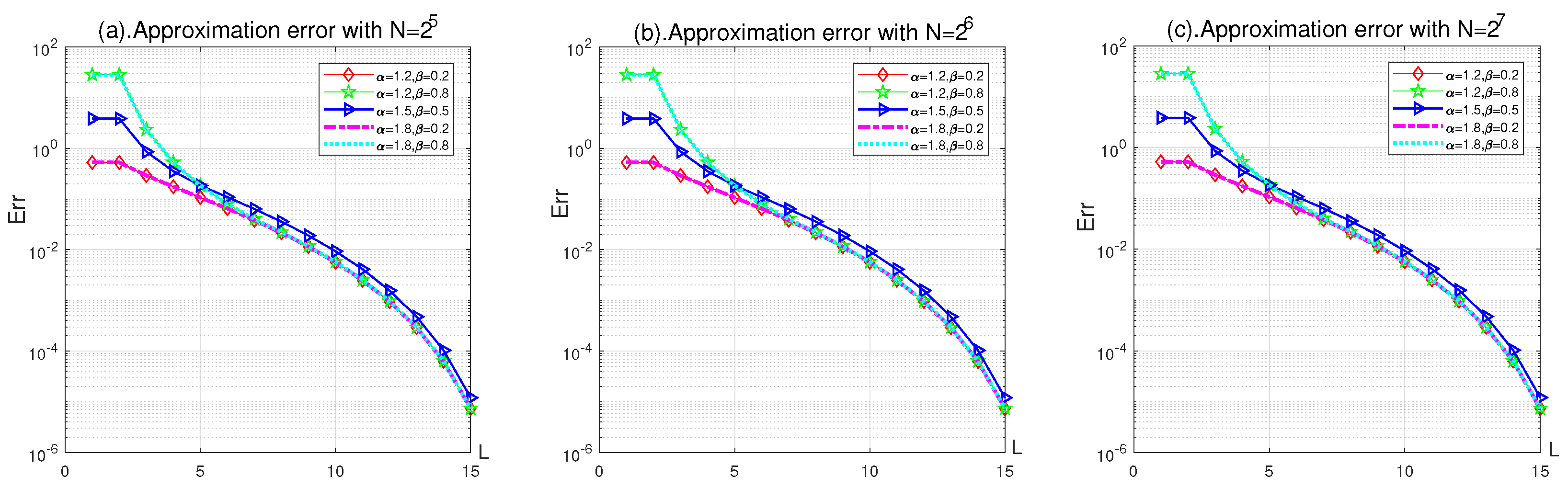
Theorem 1 gives a clear indication that ${\mathcal{M}}_L$ will approximate to $\mathcal{A}$ better and better as L gets larger and larger, and ${\mathcal{M}}_L$ will be equal to $\mathcal{A}$ if L is equal to M. In the following Figure 5 and Figure 6, we will take $M=2^4$ and depict the approximation error of ${\mathcal{M}}_L$ to $\mathcal{A}$ numerically.

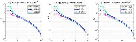
Figure 5. Approximation error of ${\mathcal{M}}_L$ to $\mathcal{A}$ with variant $\alpha ,\beta$ and N in Example 1.

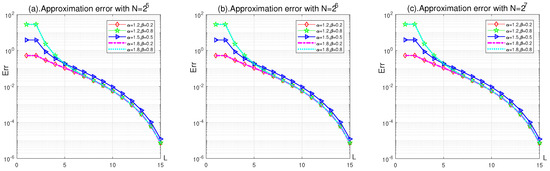
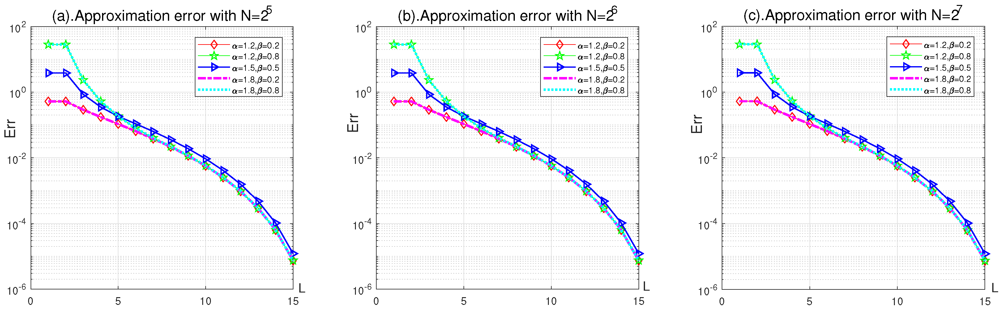
Figure 6. Approximation error of ${\mathcal{M}}_L$ to $\mathcal{A}$ with variant $\alpha ,\beta$ and N in Example 2.

Figure 5 and Figure 6 verify that the approximation error $||\mathcal{E}||{}_{\infty }$ in Theorem 1 indeed gets smaller and smaller as L gets larger and larger. Furthermore, Figure 5 and Figure 6 also reveal the fact that even with variant $\alpha ,\beta$ and N, the error between ${\mathcal{M}}_L$ and $\mathcal{A}$ can always stay smaller than 1 as long as L is larger than 4.

Similar to the contents of the bi-diagonal preconditioner in Ref. [54], in order to analyze the preconditioned effect of block L-diagonal preconditioner, we consider the spectral property of the preconditioned coefficient matrix ${\mathcal{M}}_L^{-1}\mathcal{A}$ as follows.

Theorem 2.

All eigenvalues of ${\mathcal{M}}_L^{-1}\mathcal{A}$ are approximate to 1.

Proof. 

Let ∗ represent the nonzero block matrix. Then we obtain

$${\mathcal{M}}_L^{-1}\mathcal{A}=\left(\begin{array}{ccccccc}{I}_N& O& \cdots & \cdots & \cdots & \cdots & O\\ O& I_N& \cdots & \cdots & \cdots & \cdots & O\\ ⋮& \ddots & \ddots & \ddots & \ddots & ⋮& ⋮\\ O& \ddots & O& I_N& O& ⋮& ⋮\\ \ast & O& \ddots & \ddots & \ddots & \cdots & O\\ ⋮& \ddots & \ddots & \ddots & \ddots & \ddots & ⋮\\ \ast & \cdots & \ast & O& \cdots & O& I_N\end{array}\right),$$

This indicates that the eigenvalues of ${\mathcal{M}}_L^{-1}\mathcal{A}$ are all approximate to 1. □

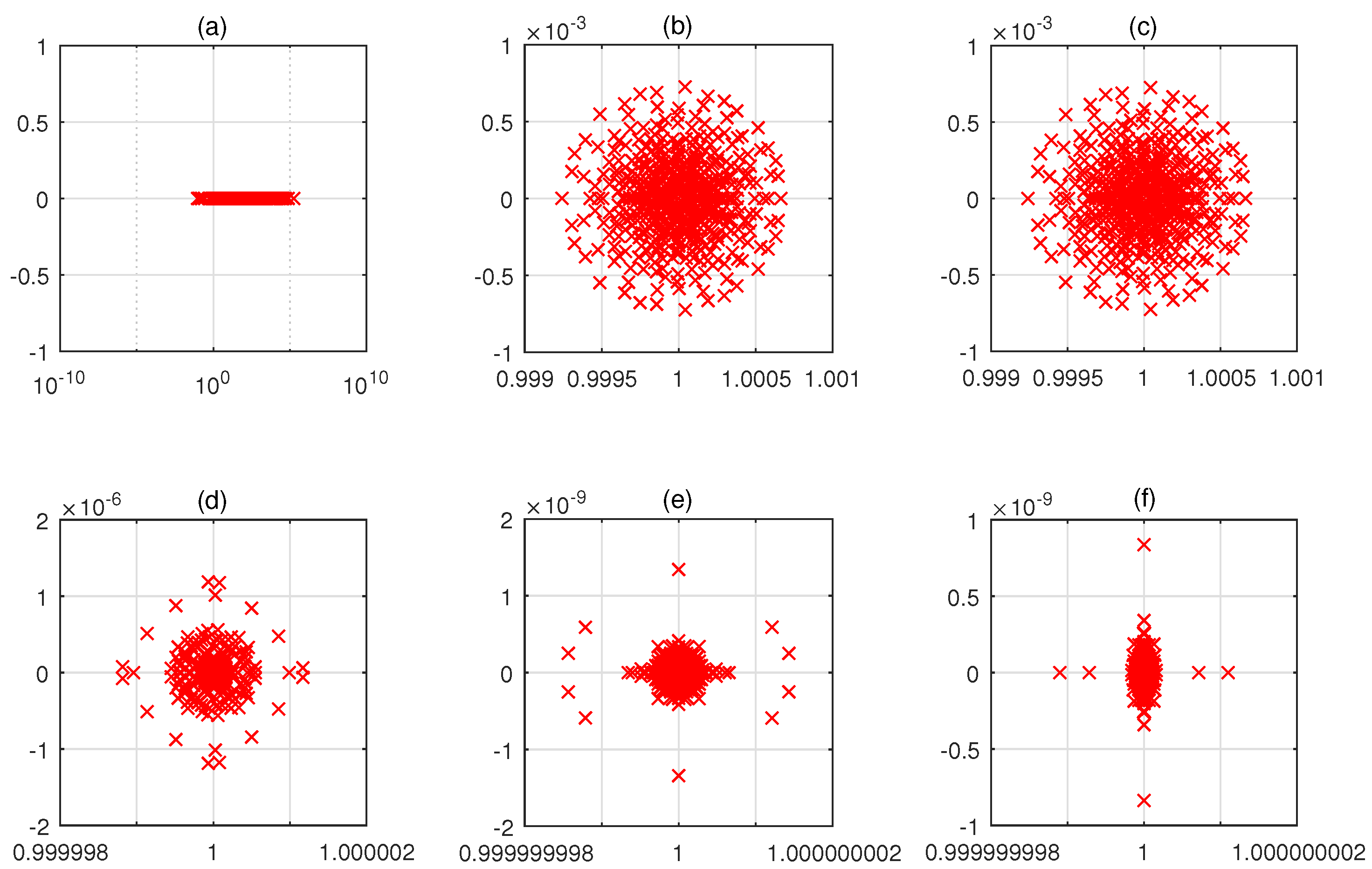
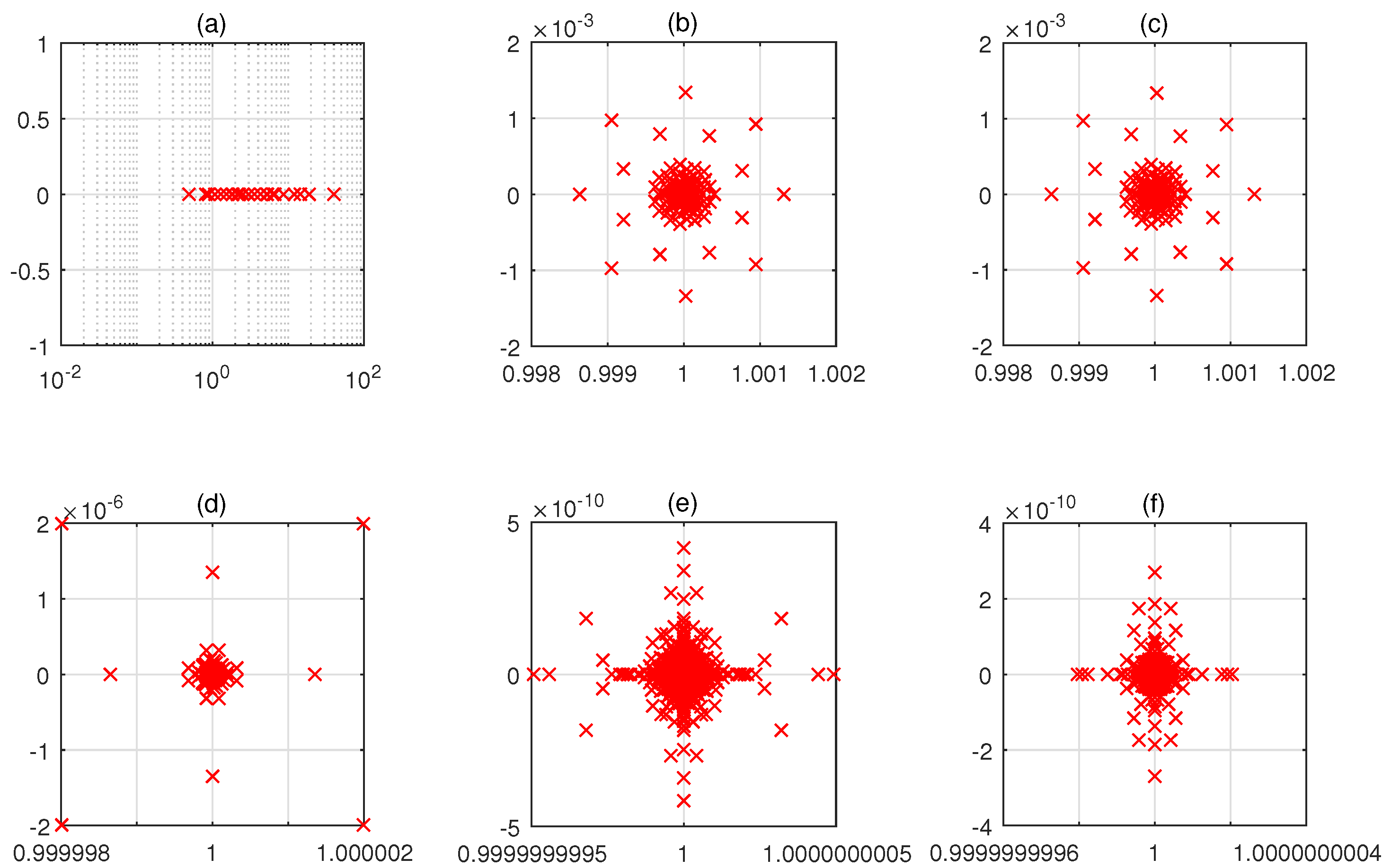
From Theorem 2 and the following Figure 7 and Figure 8, we can observe that the block L-diagonal preconditioner ${\mathcal{M}}_L$ can indeed make the eigenvalues of the coefficient matrix $\mathcal{A}$ cluster around 1. Besides, Figure 7 and Figure 8 further exhibit numerically that the spectral distribution of ${\mathcal{M}}_L^{-1}\mathcal{A}$ clusters closer to 1 as L gets larger and larger.

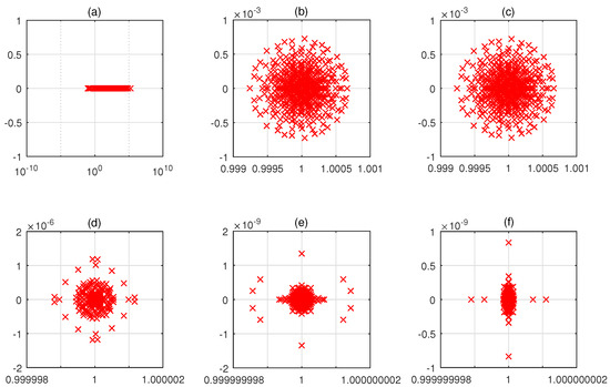
Figure 7. Spectral distribution of the coefficient matrices, where (a) is of $\mathcal{A}$ with $\alpha =1.2,\beta =0.8$, $M=2^4$, $N=2^5$ in Example 1, and (b–f) is of ${\mathcal{M}}_L^{-1}\mathcal{A}$ with $L=1,2,5,8,10$, respectively.

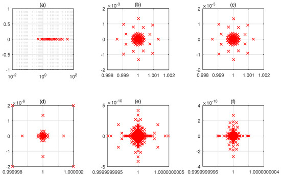
Figure 8. Spectral distribution of the coefficient matrices, where (a) is of $\mathcal{A}$ with $\alpha =1.8,\beta =0.2$, $M=2^4$, $N=2^5$ in Example 2, and (b–f) is of ${\mathcal{M}}_L^{-1}\mathcal{A}$ with $L=1,2,5,8,10$, respectively.

4. Numerical Examples

In this section, we present two examples to verify the effectiveness of the block L-diagonal preconditioner for solving the Galerkin–Legendre spectral all-at-once system originating from Equation (1) with nonsmooth solution in temporal space [29]. To solve the preconditioned system by the PGMRES method (right-preconditioned GMRES), we use the built-in function “∖” in MATLAB to calculate ${\mathcal{M}}_L^{-1}$ and the iterative process of PGMRES may terminate if the relative residual error satisfies $res=\parallel b-\mathcal{A}u\parallel /\parallel b\parallel <{10}^{-8}$ or the iteration number is more than 1000. The initial guess of PGMRES is set as zero vector and for simplicity, “TS” represents that we solve the linear system in timing-step scheme by using MINRES method, “PGMRES (L = 0)” means that we use GMRES without preconditioner and “PGMRES (L = 1, 2, 5, 8, 10)” exhibit that we utilize PGMRES with preconditioner ${\mathcal{M}}_L$ (L is equal to $1,2,5,8,10$) to solve the all-at-once system, respectively. Moreover, “cond” stands for the condition number of the coefficient matrix, “Its” and “Time” express the iterative time and total cost in PGMRES, and “†” represents that PGMRES can not converge within 1000 iterations. The unit of time is seconds.

All experiments are conducted in double precision arithmetic on Windows 10 and MATLAB R2017a with Intel (R) Core (TM) i7-8750H CPU@2.2GHz, using a PC with 8GB of memory.

Example 1.

Consider the Galerkin–Legendre spectral all-at-once system arising from the following fractional equation

$$\begin{array}{c}\left\{\begin{array}{c}{}_0^c{D}_t^{\beta }u(x,t)=\frac{{\partial }^{\alpha }u(x,t)}{\partial {|x|}^{\alpha }}+g(x,t),(x,t)\in (-1,1)\times (0,1],\hfill \\ u(x,0)=0,x\in (-1,1),\hfill \\ u(-1,t)=u(1,t)=0,t\in (0,1],\hfill \end{array}\right.\hfill \end{array}$$

(8)

where

$$\begin{array}{c}g(x,t)=\frac{1}{2cos(\pi \beta /2)}(\frac{\Gamma (3)}{\Gamma (3-\beta )}(x^{2-\beta }+{(1-x)}^{2-\beta })\hfill \\ \hspace{1em}\hspace{1em}-\frac{\Gamma (4)}{\Gamma (4-\beta )}(x^{3-\beta }+{(1-x)}^{3-\beta })+\frac{\Gamma (5)}{\Gamma (5-\beta )}(x^{4-\beta }+{(1-x)}^{4-\beta })).\hfill \end{array}$$

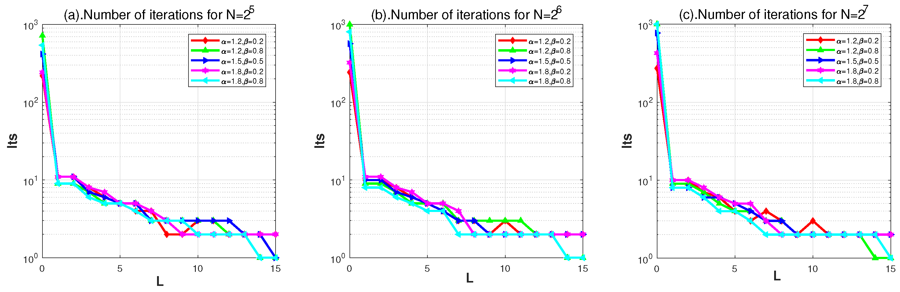
In order to investigate the effect of ${\mathcal{M}}_L$ on PGMRES, we depict the number of iterations such that $res<{10}^{-8}$ with variant L for different $\alpha ,\beta$, and N in the following Figure 9.

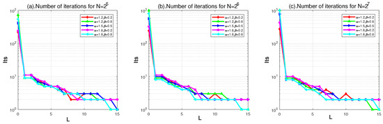
Figure 9. The number of iterations for PGMRES in Example 1 with $M=2^4$, and $L=0$ represents GMRES without the preconditioner.

Figure 9 indicates that even for different cases with various $\alpha ,\beta$, and N, PGMRES can always converge faster than GMRES. In addition, PGMRES converges faster and faster as L gets larger and larger, while the improvement of convergence is no longer significant if L is larger than 8. More detailed test results are shown in Table 1.

Table 1. Test results with different methods for Example 1, where $M=2^4$, $\gamma =1.8$.

		TS	PGMRES (L = 0)		PGMRES (L = 1)			PGMRES (L = 2)
($\mathit{\alpha }$,  $\mathit{\beta }$)	N	Time	Its	Time	Cond	Its	Time	Cond	Its	Time
(1.2, 0.2)	$2^5$	0.0467	118	0.0260	$8.0223\times {10}^1$	12	0.0624	$8.0223\times {10}^1$	12	0.0684
	$2^6$	0.1326	129	1.1481	$7.9859\times {10}^1$	12	0.1872	$7.9859\times {10}^1$	12	0.2004
	$2^7$	1.2871	147	11.4620	$7.9805\times {10}^1$	12	2.0208	$7.9805\times {10}^1$	12	2.0796
(1.2, 0.8)	$2^5$	0.0457	†	—	$5.6772\times {10}^{16}$	46	0.2397	$5.6772\times {10}^{16}$	46	0.2623
	$2^6$	0.1328	†	—	$5.6676\times {10}^{16}$	59	0.9206	$5.6676\times {10}^{16}$	59	0.9852
	$2^7$	1.2962	†	—	$5.6694\times {10}^{16}$	50	8.4211	$5.6694\times {10}^{16}$	50	8.6656
(1.5, 0.5)	$2^5$	0.0471	242	0.4841	$3.9448\times {10}^{12}$	44	0.2289	$3.9448\times {10}^{12}$	44	0.2508
	$2^6$	0.1504	284	2.5277	$3.9432\times {10}^{12}$	44	0.6865	$3.9432\times {10}^{12}$	44	0.7349
	$2^7$	1.2913	334	18.7640	$3.9429\times {10}^{12}$	44	7.4096	$3.9429\times {10}^{12}$	44	7.6252
(1.8, 0.2)	$2^5$	0.0500	250	0.5007	$1.4506\times {10}^{11}$	26	0.1301	$1.4506\times {10}^{11}$	26	0.1483
	$2^6$	0.1355	337	2.9993	$1.4676\times {10}^{11}$	24	0.3745	$1.4676\times {10}^{11}$	24	0.4018
	$2^7$	1.2899	452	21.9922	$1.4720\times {10}^{11}$	23	3.8733	$1.4720\times {10}^{11}$	23	3.9859
(1.8, 0.8)	$2^5$	0.0496	†	—	$4.2228\times {10}^{17}$	41	0.2132	$4.2228\times {10}^{17}$	41	0.2338
	$2^6$	0.1311	†	—	$4.2250\times {10}^{17}$	41	0.6397	$4.2250\times {10}^{17}$	41	0.6847
	$2^7$	1.2867	†	—	$4.2255\times {10}^{17}$	40	6.7361	$4.2255\times {10}^{17}$	40	6.9324
		PGMRES ($\mathit{L}$= 5)			PGMRES ($\mathit{L}$= 8)			PGMRES ($\mathit{L}$= 10)
($\mathit{\alpha }$,  $\mathit{\beta }$)	$\mathit{N}$	$\mathit{Cond}$	$\mathit{Its}$	$\mathit{Time}$	$\mathit{Cond}$	$\mathit{Its}$	$\mathit{Time}$	$\mathit{Cond}$	$\mathit{Its}$	$\mathit{Time}$
(1.2, 0.2)	$2^5$	$1.3838\times {10}^1$	7	0.0441	2.2266	4	0.0364	1.3307	4	0.0484
	$2^6$	$1.3787\times {10}^1$	7	0.1253	$2.2244$	4	0.1024	$1.3304$	3	0.1113
	$2^7$	$1.3779\times {10}^1$	7	1.2747	$2.2243$	4	0.9460	$1.3304$	3	1.0827
(1.2, 0.8)	$2^5$	$1.5818\times {10}^{13}$	7	0.0441	$3.4837\times {10}^8$	5	0.0459	$1.7446\times {10}^3$	5	0.0484
	$2^6$	$1.5824\times {10}^{13}$	7	0.1253	$3.5053\times {10}^8$	5	0.1281	$1.7210\times {10}^3$	4	0.1485
	$2^7$	$1.5838\times {10}^{13}$	7	1.2745	$3.5135\times {10}^8$	6	1.4013	$1.7159\times {10}^3$	4	1.4410
(1.5,0.5)	$2^5$	$1.9160\times {10}^7$	7	0.0440	$2.2722$	4	0.0365	$1.0929$	4	0.0483
	$2^6$	$1.9241\times {10}^7$	7	0.1252	$2.2805$	4	0.1026	$1.0929$	4	0.1486
	$2^7$	$1.9262\times {10}^7$	7	1.2746	$2.2826$	4	0.9461	$1.0929$	4	1.4410
(1.8, 0.2)	$2^5$	$1.4985\times {10}^3$	7	0.0442	$1.4292$	4	0.0365	$1.0875$	4	0.0485
	$2^6$	$1.5065\times {10}^3$	7	0.1255	$1.4298$	4	0.1025	$1.0876$	4	0.1486
	$2^7$	$1.5086\times {10}^3$	7	1.2745	$1.4299$	4	0.9461	$1.0876$	4	1.4411
(1.8, 0.8)	$2^5$	$2.8177\times {10}^{14}$	6	0.0378	$5.0197\times {10}^{10}$	4	0.0366	$1.9088\times {10}^7$	4	0.0485
	$2^6$	$2.8207\times {10}^{14}$	6	0.1074	$5.0249\times {10}^{10}$	4	0.1026	$1.9117\times {10}^7$	4	0.1485
	$2^7$	$2.8347\times {10}^{14}$	6	1.0990	$5.0262\times {10}^{10}$	4	0.9462	$1.9125\times {10}^7$	3	1.0873

As can be seen from Table 1, for the improvement of illness in the coefficient matrix, performance of ${\mathcal{M}}_L$ gets better and better as L increases. Additionally, Table 1 shows that GMRES cannot always converge within the specified 1000 iterations, while PGMRES can always converge, and this indicates that the preconditioner ${\mathcal{M}}_L$ is effective for solving the all-at-once system (5). From Table 1, we can observe that PGMRES (L = 1, 2) usually converges within 60 iterations while PGMRES (L = 5) can converge within 8 iterative steps, PGMRES (L = 8) can converge within 6 iterations, and PGMRES (L = 10) can converge within 5 iterations. This informs us that reduction of the number of iterations in PGMRES is not obvious as L turns larger than 8 or smaller than 5. Accordingly, cost time of PGMRES (L = 5) and PGMRES (L = 8) are usually less than that of PGMRES with other L and this phenomenon is basically unaffected by the variance of $\alpha ,\beta$, and N. On the other hand, Table 1 also manifests that the total cost of TS is always more than that of PGMRES (L = 5) and PGMRES (L = 8), which reveals the fact that to solve TSFDE in this example, using PGMRES with preconditioner ${\mathcal{M}}_L$ to solve the all-at-once system is more efficient than using MINRES to solve the traditional timing-step system, and L = 5–8 is appropriate.

Next, in order to further investigate the effect of parameter L on the application of ${\mathcal{M}}_L$ for different cases with various M, we take $N=2^5$ and show the test results in the following Table 2.

Table 2. Test results with different methods for Example 1, where $N=2^5$, $\gamma =5$.

		TS	PGMRES (L = 0)		PGMRES (L = 1)			PGMRES (L = 2)
($\mathit{\alpha }$,  $\mathit{\beta }$)	M	Time	Its	Time	Cond	Its	Time	Cond	Its	Time
(1.2, 0.2)	$2^3$	0.0061	111	0.0777	$6.2833\times {10}^1$	7	0.0063	$6.2833\times {10}^1$	7	0.0091
	$2^4$	0.0321	219	0.4380	$2.6591\times {10}^2$	11	0.0572	$2.6591\times {10}^2$	11	0.0637
	$2^5$	0.1826	393	3.5370	$2.2167\times {10}^6$	16	0.2512	$2.2167\times {10}^6$	16	0.2703
(1.2, 0.8)	$2^3$	0.0073	325	0.2279	$4.9657$	6	0.0054	$4.9657$	6	0.0079
	$2^4$	0.0327	720	1.9477	$2.0546\times {10}^5$	9	0.0466	$2.0546\times {10}^5$	9	0.0516
	$2^5$	0.1831	†	—	$1.0076\times {10}^{16}$	66	1.0363	$1.0076\times {10}^{16}$	66	1.1201
(1.5, 0.5)	$2^3$	0.0075	216	0.1520	$6.5755\times {10}^2$	6	0.0057	$6.5755\times {10}^2$	6	0.0078
	$2^4$	0.0349	417	0.8970	$7.5937\times {10}^3$	11	0.0573	$7.5937\times {10}^3$	11	0.0639
	$2^5$	0.1858	958	9.4513	$1.2785\times {10}^{12}$	19	0.2984	$1.2785\times {10}^{12}$	19	0.3231
(1.8, 0.2)	$2^3$	0.0056	123	0.0867	$2.3394$	5	0.0047	$2.3394$	5	0.0056
	$2^4$	0.0323	243	0.4986	$2.0477\times {10}^6$	11	0.0573	$2.0477\times {10}^6$	11	0.0636
	$2^5$	0.1722	†	—	$1.4489\times {10}^{13}$	66	1.0371	$1.4489\times {10}^{13}$	66	1.1206
(1.8, 0.8)	$2^3$	0.0070	260	0.1822	$1.8289\times {10}^1$	5	0.0045	$1.8289\times {10}^1$	5	0.0059
	$2^4$	0.0328	542	1.3312	$1.7490\times {10}^4$	9	0.0467	$1.7490\times {10}^4$	9	0.0519
	$2^5$	0.1744	†	—	$1.3829\times {10}^{12}$	14	0.2199	$1.3829\times {10}^{12}$	14	0.2376
		PGMRES ($\mathit{L}$= 3)			PGMRES ($\mathit{L}$= 5)			PGMRES ($\mathit{L}$= 8)
($\mathit{\alpha }$,  $\mathit{\beta }$)	$\mathit{N}$	$\mathit{Cond}$	$\mathit{Its}$	$\mathit{Time}$	$\mathit{Cond}$	$\mathit{Its}$	$\mathit{Time}$	$\mathit{Cond}$	$\mathit{Its}$	$\mathit{Time}$
(1.2, 0.2)	$2^3$	6.8387	5	0.0071	1.1243	2	0.0037	1.0000	1	0.0059
	$2^4$	$9.2652\times {10}^1$	8	0.0480	$9.1453$	5	0.0322	$1.3550$	2	0.0330
	$2^5$	$3.3225\times {10}^5$	12	0.2112	$9.9571\times {10}^3$	9	0.1647	$1.3125\times {10}^1$	7	0.1813
(1.2, 0.8)	$2^3$	$1.4280$	5	0.0073	$1.0102$	3	0.0059	$1.0000$	1	0.0061
	$2^4$	$2.6038\times {10}^4$	7	0.0423	$5.9225\times {10}^2$	5	0.0325	$2.5358$	3	0.0376
	$2^5$	$2.5282\times {10}^{15}$	22	0.3876	$2.3686\times {10}^{14}$	9	0.1649	$7.9200\times {10}^{12}$	6	0.1659
(1.5, 0.5)	$2^3$	$5.1720\times {10}^1$	4	0.0057	$1.5032$	3	0.0056	$1.0000$	1	0.0063
	$2^4$	$8.8596\times {10}^2$	7	0.0425	$1.4193\times {10}^1$	5	0.0325	$1.0610$	3	0.0379
	$2^5$	$4.1838\times {10}^{11}$	13	0.2289	$5.7728\times {10}^{10}$	9	0.1646	$2.3331\times {10}^9$	6	0.1657
(1.8, 0.2)	$2^3$	$1.1211$	4	0.0059	$1.0033$	2	0.0039	$1.0000$	1	0.0060
	$2^4$	$2.3756\times {10}^5$	8	0.0483	$3.2439\times {10}^3$	5	0.0322	$1.8113$	3	0.0377
	$2^5$	$4.0994\times {10}^{12}$	33	0.5809	$7.3077\times {10}^{11}$	9	0.1647	$3.0587\times {10}^{10}$	7	0.1816
(1.8, 0.8)	$2^3$	$2.5431$	4	0.0059	$1.0492$	3	0.0057	$1.0000$	1	0.0063
	$2^4$	$2.0015\times {10}^3$	6	0.0362	$3.8250\times {10}^1$	5	0.0323	$1.1927$	3	0.0377
	$2^5$	$4.2365\times {10}^{11}$	11	0.1941	$4.7639\times {10}^{10}$	7	0.1281	$2.2020\times {10}^9$	6	0.1555

Table 2 states that for different cases with various $\alpha ,\beta$, and M, ${\mathcal{M}}_L$ is always effective. Furthermore, ${\mathcal{M}}_L$ is almost equally effective for the cases with different $\alpha ,\beta$ while for the case with large M, the effectiveness of ${\mathcal{M}}_L$ is usually more significant. As can be seen from Table 2, for the effectiveness of ${\mathcal{M}}_L$ on PGMRES (L), the selection of parameter L is not significantly affected by the temporal discrete size M, and for different cases with various M, preconditioner ${\mathcal{M}}_L$ turns out to be more efficient as the parameter L gets around 5 and 8. Therefore, for the sake of an overall performance, L does not need to be taken too large and L = 5–8 is usually appropriate.

In addition, in order to illustrate that the numerical solution obtained from the Galerkin–Legendre spectral all-at-once system is reasonable for Equation (1), we depict the numerical solutions for Equation (8) in Figure 10. We note that analytical solution in Equation (8) is difficult to obtain, hence we here consider the numerical solution under ra efined grid as the exact solution, and we also compare the numerical solutions obtained by different methods for Equation (8). Besides, in Figure 10, TS represents solving the timing-step scheme by MINRES and AAO(L) stands for solving the all-at-once scheme by PGMRES with preconditioner ${\mathcal{M}}_L$. Colors from light to dark represent the graded temporal mesh divided from 0 to 1.

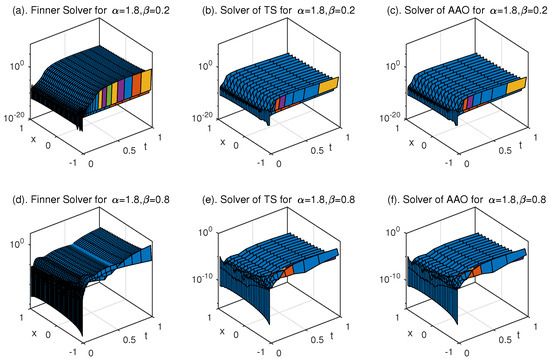
Figure 10. Solutions for Equation (8), where (a) is for $\alpha =1.8,\beta =0.2$ with $M=2^5,N=2^6$, (b,c) are for $\alpha =1.8,\beta =0.2$ with $M=2^4,N=2^5$, (d) is for $\alpha =1.8,\beta =0.8$ with $M=2^5,N=2^6$, and (e,f) are for $\alpha =1.8,\beta =0.8$ with $M=2^4,N=2^5$.

As can be seen from Figure 10, the numerical solution obtained by using AAO is similar to that obtained by using TS, and they are both approximated to the numerical solution under the refined grid. Therefore, the numerical solution obtained from the Galerkin–Legendre spectral all-at-once system is reasonable for Equation (8).

Example 2.

Consider the Galerkin–Legendre spectral all-at-once system arising from the following fractional equation

$$\begin{array}{c}\left\{\begin{array}{c}{}_0^c{D}_t^{\beta }u(x,t)=0.5\frac{{\partial }^{\alpha }u(x,t)}{\partial {|x|}^{\alpha }}+g(x,t),(x,t)\in (0,2)\times (0,1],\hfill \\ u(x,0)=x^2{(1-x)}^2,x\in (0,2),\hfill \\ u(-1,t)=u(1,t)=0,t\in (0,1],\hfill \end{array}\right.\hfill \end{array}$$

(9)

where

$$\begin{array}{c}g(x,t)=\frac{1}{2cos(\pi \beta /2)}(\frac{4\Gamma (3)}{\Gamma (3-\beta )}({(1+x)}^{2-\beta }+{(1-x)}^{2-\beta })\hfill \\ -\frac{4\Gamma (4)}{\Gamma (4-\beta )}({(1+x)}^{3-\beta }+{(1-x)}^{3-\beta })+\frac{\Gamma (5)}{\Gamma (5-\beta )}({(1+x)}^{4-\beta }+{(1-x)}^{4-\beta })).\hfill \end{array}$$

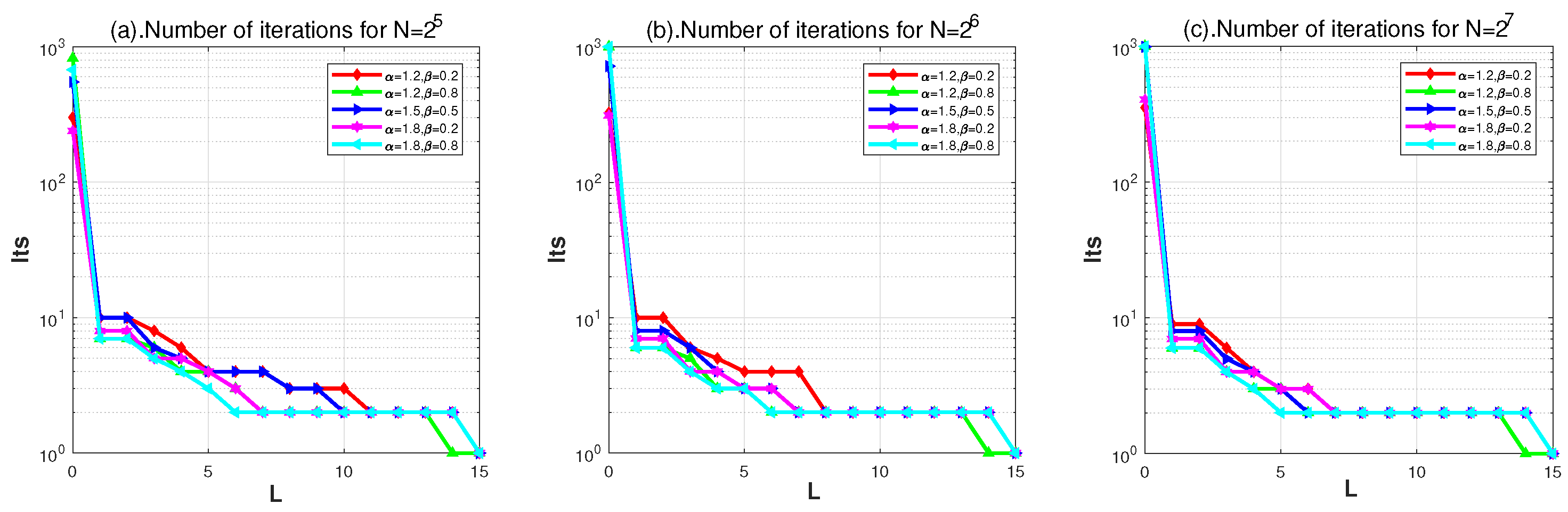
Firstly, we take $M=2^4$, $N=2^5,2^6,2^7$ with variant L to explore the effect of preconditioner ${\mathcal{M}}_L$ on the number of iterations for PGMRES in the following Figure 11.

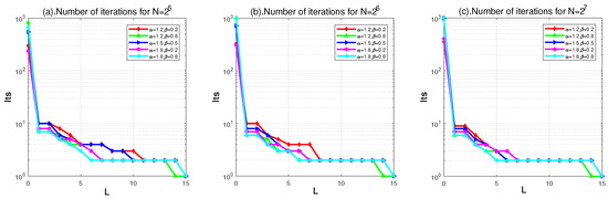
Figure 11. The number of iterations for PGMRES in Example 2 with $M=2^4$, and $L=0$ represents GMRES without the preconditioner.

Figure 11 claims that PGMRES always converges faster than GMRES, and PGMRES converges faster and faster as L gets larger and larger. Nevertheless, the number of iterations in PGMRES barely decreases as L grows larger than 8, and this phenomenon is barely affected by the variance of $\alpha ,\beta$, and N. More detailed test results about the condition number of the coefficient matrix and total cost in the solving with different solvers are shown in Table 3.

Table 3. Test results with different methods for Example 2, where $M=2^4$, $\gamma =1.8$.

		$\mathbf{TS}$	PGMRES (L = 0)		PGMRES (L = 1)			PGMRES (L = 2)
($\mathit{\alpha }$,  $\mathit{\beta }$)	N	Time	Its	Time	Cond	Its	Time	Cond	Its	Time
(1.2, 0.2)	$2^5$	0.0451	†	—	$3.2603\times {10}^{20}$	29	0.1508	$3.2603\times {10}^{20}$	29	0.1656
	$2^6$	0.1136	†	—	$3.0657\times {10}^{20}$	20	0.3121	$3.0657\times {10}^{20}$	20	0.3341
	$2^7$	1.1024	†	—	$3.0489\times {10}^{20}$	30	5.0520	$3.0489\times {10}^{20}$	30	5.1990
(1.2, 0.8)	$2^5$	0.0390	†	—	$4.4239\times {10}^{17}$	13	0.0679	$4.4239\times {10}^{17}$	13	0.0741
	$2^6$	0.1137	†	—	$4.5075\times {10}^{17}$	13	0.2029	$4.5075\times {10}^{17}$	13	0.2173
	$2^7$	1.1023	929	25.6340	$4.5332\times {10}^{17}$	13	2.1893	$4.5332\times {10}^{17}$	13	2.2529
(1.5, 0.5)	$2^5$	0.0392	329	0.6583	$1.5184\times {10}^{15}$	13	0.0677	$1.5184\times {10}^{15}$	13	0.0743
	$2^6$	0.0960	386	3.4356	$1.4644\times {10}^{15}$	12	0.1875	$1.4644\times {10}^{15}$	12	0.2004
	$2^7$	0.9211	451	21.8463	$1.4507\times {10}^{15}$	12	2.0209	$1.4507\times {10}^{15}$	12	2.0799
(1.8, 0.2)	$2^5$	0.0263	172	0.3441	$3.4310$	9	0.0468	$3.4310$	9	0.0513
	$2^6$	0.0601	222	1.9758	$3.4307$	8	0.1249	$3.4307$	8	0.1336
	$2^7$	0.5567	295	17.0707	$3.4306$	8	1.3473	$3.4306$	8	1.3865
(1.8, 0.8)	$2^5$	0.0340	†	—	$2.7782\times {10}^{17}$	11	0.0574	$2.7782\times {10}^{17}$	11	0.0627
	$2^6$	0.0778	591	5.2599	$2.7806\times {10}^{17}$	11	0.1717	$2.7806\times {10}^{17}$	11	0.1838
	$2^7$	0.9292	†	—	$2.7822\times {10}^{17}$	11	1.8526	$2.7822\times {10}^{17}$	11	1.9663
		PGMRES ($\mathit{L}$= 5)			PGMRES ($\mathit{L}$= 8)			PGMRES ($\mathit{L}$= 10)
($\mathit{\alpha }$,  $\mathit{\beta }$)	$\mathit{N}$	$\mathit{Cond}$	$\mathit{Its}$	$\mathit{Time}$	$\mathit{Cond}$	$\mathit{Its}$	$\mathit{Time}$	$\mathit{Cond}$	$\mathit{Its}$	$\mathit{Time}$
(1.2, 0.2)	$2^5$	$7.3722\times {10}^{17}$	7	0.0442	$7.6596\times {10}^{13}$	4	0.0367	$1.7423\times {10}^{10}$	3	0.0363
	$2^6$	$5.8231\times {10}^{17}$	6	0.1074	$7.4080\times {10}^{13}$	3	0.0769	$1.7221\times {10}^{10}$	3	0.1113
	$2^7$	$1.9544\times {10}^{17}$	6	1.0927	$7.3371\times {10}^{13}$	3	0.7006	$1.7207\times {10}^{10}$	3	1.0801
(1.2, 0.8)	$2^5$	$4.1243\times {10}^{14}$	6	0.0379	$1.4035\times {10}^{11}$	5	0.0455	$1.3875\times {10}^8$	4	0.0485
	$2^6$	$4.2099\times {10}^{14}$	6	0.1076	$1.4368\times {10}^{11}$	4	0.1024	$1.4261\times {10}^8$	4	0.1486
	$2^7$	$4.2358\times {10}^{14}$	6	1.0927	$1.4468\times {10}^{11}$	2	0.4716	$1.4374\times {10}^8$	3	1.0804
(1.5, 0.5)	$2^5$	$3.3323\times {10}^{10}$	6	0.0381	$3.9761\times {10}^1$	4	0.0367	$2.1642$	3	0.0365
	$2^6$	$3.2233\times {10}^{10}$	5	0.0896	$4.0209\times {10}^1$	4	0.1024	$2.1625$	3	0.1113
	$2^7$	$3.1964\times {10}^{10}$	5	0.9105	$4.0327\times {10}^1$	4	0.9342	$2.1621$	2	0.7203
(1.8, 0.2)	$2^5$	$1.6948$	4	0.0253	$1.2017$	3	0.0274	$1.0864$	3	0.0365
	$2^6$	$1.6948$	3	0.0538	$1.2016$	2	0.0521	$1.0864$	2	0.0742
	$2^7$	$1.6947$	3	0.5464	$1.2016$	2	0.4717	$1.0864$	2	0.7204
(1.8, 0.8)	$2^5$	$1.3425\times {10}^{14}$	5	0.0317	$1.1693\times {10}^{10}$	4	0.0369	$1.3003\times {10}^6$	3	0.0363
	$2^6$	$1.3446\times {10}^{14}$	4	0.0716	$1.1716\times {10}^{10}$	3	0.0767	$1.3038\times {10}^6$	2	0.0742
	$2^7$	$1.3452\times {10}^{14}$	5	0.9102	$1.1722\times {10}^{10}$	2	0.4716	$1.3048\times {10}^6$	2	0.7206

Table 3 recounts that the condition number of the coefficient matrix is reduced and the number of iterations in PGMRES (L) is always less than that in GMRES. This explicates that the preconditioner ${\mathcal{M}}_L$ is always effective for solving the all-at-once system (5). Besides, the number of iterations in PGMRES (L) gets smaller and smaller as L gets larger and larger while the total cost in PGMRES (L) does not always decrease as L increases. This phenomenon propagates the fact that an appropriate value of L is important for the application of ${\mathcal{M}}_L$ in PGMRES (L). Based on the test results in Table 3, we see that the total cost of PGMRES (L = 5) and PGMRES (L = 8) are far less than that of TS and other PGMRES, which suggests that L = 5–8 is appropriate.

In order to further explore the effect of L on the application of preconditioner ${\mathcal{M}}_L$ for different cases with various M, we take $N=2^5$ and present the detailed test results in Table 4.

Table 4. Test results with different methods for Example 2, where $N=2^5$, $\gamma =5$.

		$\mathbf{TS}$	PGMRES (L = 0)		PGMRES (L = 1)			PGMRES (L = 2)
($\mathit{\alpha }$,  $\mathit{\beta }$)	M	Time	Its	Time	Cond	Its	Time	Cond	Its	Time
(1.2, 0.2)	$2^3$	0.0073	167	0.1336	$1.5765\times {10}^1$	6	0.0061	$1.5765\times {10}^1$	6	0.0090
	$2^4$	0.0318	301	0.9280	$1.8061\times {10}^6$	10	0.0559	$1.8061\times {10}^6$	10	0.0623
	$2^5$	0.1818	661	6.1404	$2.6876\times {10}^{14}$	18	0.2376	$2.6876\times {10}^{14}$	18	0.3130
(1.2, 1.8)	$2^3$	0.0079	393	0.3157	$6.2765\times {10}^1$	6	0.0059	$6.2765\times {10}^1$	6	0.0089
	$2^4$	0.0331	824	2.0452	$8.8437\times {10}^4$	7	0.0394	$8.8437\times {10}^4$	7	0.0434
	$2^5$	0.1809	†	—	$5.3936\times {10}^{12}$	12	0.1585	$5.3936\times {10}^{12}$	12	0.2083
(1.5, 0.5)	$2^3$	0.0068	265	0.2123	$4.9789\times {10}^1$	6	0.0061	$4.9789\times {10}^1$	6	0.0091
	$2^4$	0.0326	550	1.5621	$7.2266\times {10}^5$	10	0.0561	$7.2266\times {10}^5$	10	0.0623
	$2^5$	0.1792	†	—	$9.9120\times {10}^{12}$	16	0.2116	$9.9120\times {10}^{12}$	16	0.2776
(1.8, 0.2)	$2^3$	0.007	132	0.1059	$1.7026$	5	0.0050	1.7026	5	0.0075
	$2^4$	0.0311	240	0.5966	$9.5716\times {10}^1$	8	0.0449	$9.5716\times {10}^1$	8	0.0498
	$2^5$	0.1801	448	4.1666	$5.2133\times {10}^5$	12	0.1587	$5.2133\times {10}^5$	12	0.2086
(1.8, 0.8)	$2^3$	0.0074	292	0.2336	$3.0889$	4	0.0041	3.0889	4	0.0060
	$2^4$	0.0329	677	1.7383	$4.8210\times {10}^6$	7	0.0392	$4.8210\times {10}^6$	7	0.0437
	$2^5$	0.1797	†	—	$9.9986\times {10}^{12}$	11	0.1456	$9.9986\times {10}^{12}$	11	0.1916
		PGMRES ($\mathit{L}$= 3)			PGMRES ($\mathit{L}$= 5)			PGMRES ($\mathit{L}$= 8)
($\mathit{\alpha }$,  $\mathit{\beta }$)	$\mathit{N}$	$\mathit{Cond}$	$\mathit{Its}$	$\mathit{Time}$	$\mathit{Cond}$	$\mathit{Its}$	$\mathit{Time}$	$\mathit{Cond}$	$\mathit{Its}$	$\mathit{Time}$
(1.2, 0.2)	$2^3$	1.5404	4	0.0081	1.0063	3	0.0069	1.0000	1	0.0071
	$2^4$	$3.0210\times {10}^5$	8	0.0552	$8.8595\times {10}^3$	4	0.0300	$1.1853\times {10}^1$	3	0.0279
	$2^5$	$1.9206\times {10}^{14}$	12	0.2196	$4.4501\times {10}^{13}$	8	0.1536	$3.2419\times {10}^{12}$	6	0.1590
(1.2,1.8)	$2^3$	$4.5616$	4	0.0083	$1.0583$	3	0.0067	$1.0000$	1	0.0073
	$2^4$	$6.9549\times {10}^3$	6	0.0414	$2.1070\times {10}^2$	4	0.0304	$2.4209$	2	0.0213
	$2^5$	$1.6767\times {10}^{12}$	9	0.1649	$1.9169\times {10}^{11}$	6	0.1152	$9.1247\times {10}^9$	5	0.1325
(1.5, 0.5)	$2^3$	$1.8809$	4	0.0081	$1.0168$	2	0.0047	$1.0000$	1	0.0069
	$2^4$	$1.5682\times {10}^5$	6	0.0417	$6.6103\times {10}^3$	4	0.0301	$3.1226\times {10}^1$	3	0.0281
	$2^5$	$3.4526\times {10}^{12}$	11	0.2013	$4.9716\times {10}^{11}$	8	0.1539	$2.1660\times {10}^{10}$	5	0.1327
(1.8, 0.2)	$2^3$	$1.1961$	4	0.0085	$1.0155$	2	0.0051	$1.0000$	1	0.0067
	$2^4$	$3.9844$	5	0.0347	$1.1854$	4	0.0299	$1.0268$	2	0.0213
	$2^5$	$6.9959\times {10}^4$	9	0.1646	$1.5038\times {10}^3$	6	0.1150	$2.2247$	3	0.0795
(1.8, 0.8)	$2^3$	$1.2631$	3	0.0064	$1.0061$	2	0.0049	$1.0000$	1	0.0071
	$2^4$	$5.5338\times {10}^5$	5	0.0349	$1.8368\times {10}^4$	3	0.0226	$7.7079\times {10}^1$	2	0.0216
	$2^5$	$2.9805\times {10}^{12}$	8	0.1464	$3.2775\times {10}^{11}$	5	0.0960	$1.4581\times {10}^{10}$	3	0.0795

Table 4 illustrates that for different cases with various $\alpha ,\beta$, and M, ${\mathcal{M}}_L$ is always effective and for the case with large M, the effectiveness of ${\mathcal{M}}_L$ is usually significant. Besides, Table 4 also shows the effect of L on the application of ${\mathcal{M}}_L$ for different cases with various M. As is shown in Table 4, similar to the results in Table 2 of Example 1, for the effectiveness of ${\mathcal{M}}_L$ on PGMRES (L), the selection of parameter L is not significantly affected by the temporal discrete size M, and ${\mathcal{M}}_L$ is more efficient as the parameter L gets around 5 and 8. Therefore, for an overall efficiency, L need not to be taken too large and L = 5–8 is usually appropriate.

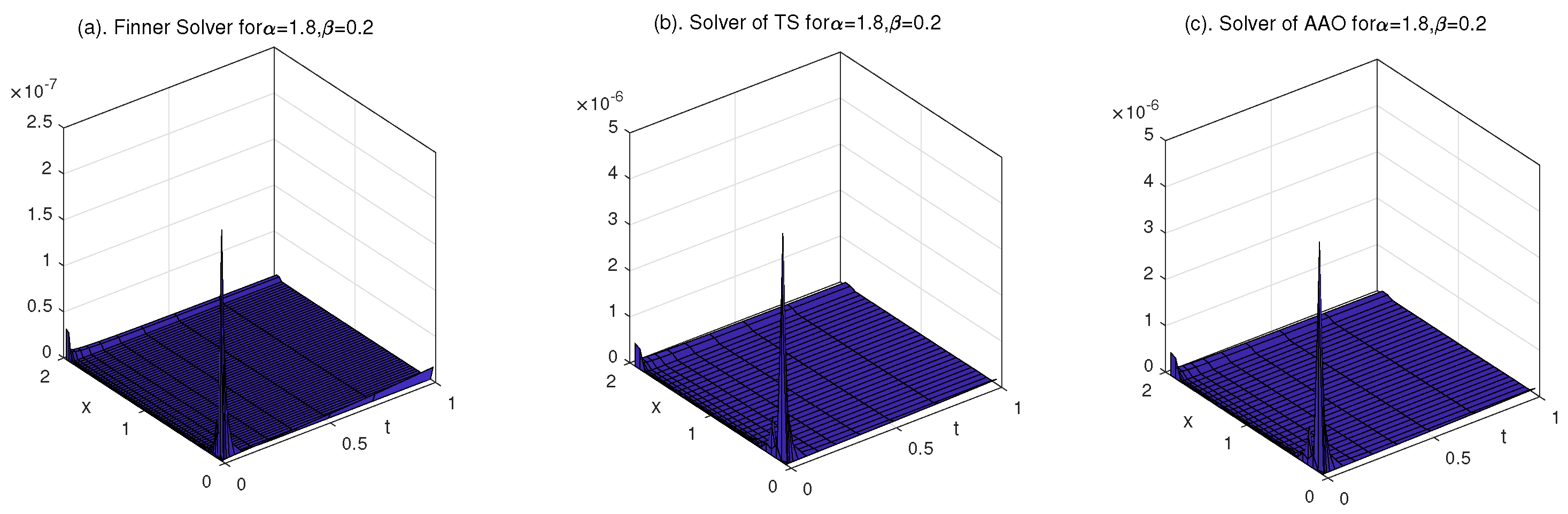
In order to explore the reliability for the numerical solution obtained from the Galerkin–Legendre spectral all-at-once system, we compare the numerical solutions for Equation (9) with different methods in the following. We note that since the analytical solution in Equation (9) is difficult to obtain, here we also use the numerical solution under refined grid as the exact solution. Solutions for Equation (9) calculated by TS and AAO(L) are present in the following Figure 12.

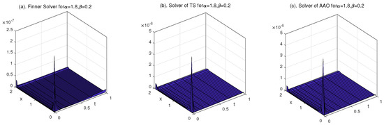
Figure 12. Solutions for Equation (9) with $\alpha =1.8,\beta =0.2$, $M=2^4$, where N is taken to be $2^7$ and $2^5$ in (a–c), respectively.

From Figure 12, we see that the numerical solutions obtained by using AAO and TS are approximate to that obtained under the refined grid. This indicates that the numerical solution obtained from the Galerkin–Legendre spectral all-at-once system is reasonable for Equation (9).

5. Conclusions

In this paper, we mainly studied an efficient way to solve Equation (1). We combined the all-at-once technique with the Galerkin–Legendre spectral method and the graded $L1$ method to solve the time-space fractional diffusion in Equation (1), and found that this scheme is more convenient for parallel computing than the traditional timing-step spectral scheme. With the observation that the coefficient matrix of the corresponding Galerkin–Legendre spectral all-at-once system is usually a block lower triangular and that the main information of the coefficient matrix is gathered in the first L-nonzero diagonal blocks, we proposed a block L-diagonal preconditioner ${\mathcal{M}}_L$ to accelerate solving the Galerkin–Legendre spectral all-at-once system. Based on the analyses of approximation error and spectral distribution of the coefficient matrix, the proposed preconditioner ${\mathcal{M}}_L$ can improve the illness of the coefficient matrix and ${\mathcal{M}}_L$ usually performs better and better as L increases. Additionally, the numerical experiments further verify the effectiveness of ${\mathcal{M}}_L$ and present the appropriate value of parameter L heuristically.

We note that the combination of the all-at-once technique with the Galerkin–Legendre spectral method and graded $L1$ method is convenient for parallel computing in solving Equation (1), and the proposed block L-diagonal preconditioner ${\mathcal{M}}_L$ can accelerate solving the corresponding Galerkin–Legendre spectral all-at-once system. However, similar to many existing works where the parameters can only be selected experimentally, in this paper, we also choose the parameter L heuristically. For future work, we will develop some adaptive techniques to set L adaptively with moderate computational cost. Furthermore, it is important to note that the time-space fractional diffusion Equation (1) considered in this paper can only be utilized to model the linear anomalous diffusion. To simulate more completed anomalous diffusion such as heterogeneous porous, non-Fickian diffusion in porous media and nonlinear diffusion in image denoising media, Equation (1) needs to be further developed into a variable-order model, distributed-order model, and nonlinear model for better application. We expect that the method proposed in this paper could be developed to handle more comprehensive models, and we plan to further explore these applications in future work.

References

- Collins, R.E. Quantum mechanics as a classical diffusion process. Found Phys. Lett. 1992, 5, 63–69. [Google Scholar] [CrossRef]
- Fan, C.; Liu, K.X.; Chen, Y.G.; Xue, Y.C.; Zhao, J.; Khudoley, A. A new modelling method of material removal profile for electrorheological polishing with a mini annular integrated electrode. J. Mater. Process. Technol. 2022, 305, 117589. [Google Scholar] [CrossRef]
- Zhao, J.; Ge, J.Y.; Khudoley, A.; Chen, H.Y. Numerical and experimental investigation on the material removal profile during polishing of inner surfaces using an abrasive rotating jet. Tribol. Int. 2024, 191, 109125. [Google Scholar] [CrossRef]
- Bouchaud, J.; Georges, A. Anomalous diffusion in disordered media: Statistical mechanisms, models and physical applications. Phys. Rep. 1990, 195, 127–293. [Google Scholar] [CrossRef]
- Sun, H.G.; Chen, W.; Li, C.P.; Chen, Y.Q. Fractional differential models for anomalous diffusion. Phys. A 2010, 389, 2719–2724. [Google Scholar] [CrossRef]
- Chaves, A.S. A fractional diffusion equation to describe Lévy flights. Phys. Lett. A 1998, 239, 13–16. [Google Scholar] [CrossRef]
- Oldham, K.B.; Spanier, J. The Fractional Calculus; Academic Press: New York, NY, USA, 1974. [Google Scholar]
- Benson, D.A.; Wheatcraft, S.W.; Meerschaert, M.M. The fractional-order governing equation of Lévy Motion. Water Resour. Res. 2000, 36, 1413–1423. [Google Scholar] [CrossRef]
- Caputo, M. Linear models of dissipation whose Q is almost frequency independent II. Geophys. J. R. Astr. Soc. 1967, 13, 529–539. [Google Scholar] [CrossRef]
- West, B.J.; Bologna, M.; Grigolini, P. Physics of Fractal Operators; Springer: New York, NY, USA, 2003. [Google Scholar]
- Diethelm, K. The Analysis of Fractional Differential Equations: An Application-Oriented Exposition Using Differential Operators of Caputo Type; Springer Science and Business Media: New York, NY, USA, 2010. [Google Scholar]
- Gorenflo, R.; Mainardi, F.; Moretti, D.; Pagnini, G.; Paradisi, P. Discrete random walk models for space-time fractional diffusion. Chem. Phys. 2002, 284, 52–541. [Google Scholar] [CrossRef]
- Metzler, R.; Klafter, J. The random walk’s guide to anomalous diffusion: A fractional dynamics approach. Phys. Rep. 2000, 339, 1–77. [Google Scholar] [CrossRef]
- Meerschaert, M.M.; Benson, D.A.; Scheffler, H.P.; Baeumer, B. Stochastic solution of space-time fractional diffusion equations. Phys. Rev. E 2002, 65, 041103. [Google Scholar] [CrossRef] [PubMed]
- Saichev, A.I.; Zaslavsky, G.M. Fractional kinetic equations: Solutions and applications. Chaos Interdiscip. J. Nonlinear Sci. 1997, 7, 753–764. [Google Scholar] [CrossRef] [PubMed]
- Scalas, E.; Gorenflo, R.; Mainardi, F. Fractional calculus and continuous-time finance. Phys. A 2000, 284, 376–384. [Google Scholar] [CrossRef]
- Obembe, A.; Hossain, M.; Abu-Khamsin, S. Variable-order derivative time fractional diffusion model for heterogeneous porous media. J. Petrol. Sci. Eng. 2017, 152, 391–405. [Google Scholar] [CrossRef]
- Liang, Y.J.; Chen, W.; Xu, W.; Sun, H.G. Distributed order Hausdorff derivative diffusion model to characterize non-Fickian diffusion in porous media. Commun. Nonlinear Sci. 2019, 70, 384–393. [Google Scholar] [CrossRef]
- Sun, H.G.; Chen, Y.Q.; Chen, W. Random-order fractional differential equation models. Signal Process. 2011, 91, 525–530. [Google Scholar] [CrossRef]
- Kumar, S.; Alam, K.; Chauhan, A. Fractional derivative based nonlinear diffusion model for image denoising. SeMA 2022, 79, 355–364. [Google Scholar] [CrossRef]
- Zhang, H.; Lv, Y. Galerkin method for a backward problem of time-space fractional symmetric diffusion equation. Symmetry 2023, 15, 1057. [Google Scholar] [CrossRef]
- Guo, B.Y.; Wang, Z.Q. Legendre-Gauss collocation methods for ordinary differential equations. Adv. Comput. Math. 2009, 30, 249–280. [Google Scholar] [CrossRef]
- Shen, J.; Tang, T.; Wang, L.L. Spectral Methods, Algorithms, Analysis, and Applications; Springer: Berlin/Heidelberg, Germany, 2011. [Google Scholar]
- Sheng, C.T.; Shen, J. A space-time Petrov-Galerkin spectral method for time fractional diffusion equation. Numer. Math. Theory Methods Appl. 2018, 11, 854–876. [Google Scholar] [CrossRef]
- Li, X.J.; Xu, X.J. A space-time spectral method for the time fractional diffusion equation. SIAM J. Numer. Anal. 2009, 47, 2108–2131. [Google Scholar] [CrossRef]
- Fakhar-Izadi, F.; Shabgard, N. Time-space spectral Galerkin method for time-fractional fourth-order partial differential equations. J. Appl. Math. Comput. 2022, 68, 4253–4272. [Google Scholar] [CrossRef]
- Lin, Y.; Xu, C. Finite difference/spectral approximations for the time-fractional diffusion equation. J. Comput. Phys. 2007, 225, 1533–1552. [Google Scholar] [CrossRef]
- Ye, X.; Xu, C. Spectral optimization methods for the time fractional diffusion inverse problem. Numer. Math. Theory Methods Appl. 2013, 6, 499–519. [Google Scholar]
- Zaky, M.A.; Hendy, A.S.; Macias-Diaz, J.E. Semi-implicit Galerkin-legendre spectral schemes for nonlinear time-space fractional diffusion-reaction equations with smooth and nonsmooth solutions. J. Sci. Comput. 2000, 82, 1–27. [Google Scholar] [CrossRef]
- Zaky, M.A.; Hendy, A.S. Convergence analysis of an L1-continuous Galerkin method for nonlinear time-space fractional Schrodinger equation. Int. J. Comput. Math. 2021, 98, 1420–1437. [Google Scholar] [CrossRef]
- Zayernouri, M.; Karniadakis, G.E. Discontinuous spectral element methods for time-and space-fractional advection equations. SIAM J. Sci. Comput. 2014, 36, B684–B707. [Google Scholar] [CrossRef]
- Hu, C.; Lv, S.J.; Chen, W.P. Spectral methods for the time fractional diffusion-wave equation in a semi-infinite channel. Comput. Math. Appl. 2016, 9, 1818–1830. [Google Scholar]
- Huang, Y.; Skandari, M.H.N.; Mohammadizadeh, F.; Tehrani, H.A.; Georgiev, S.G.; Tohidi, E.; Shateyi, S. Space-time spectral collocation method for solving Burgers equations with the convergence analysis. Symmetry 2019, 11, 1439. [Google Scholar] [CrossRef]
- Wang, Y.; Cai, M. Finite difference schemes for time-space fractional diffusion equations in one-and two-dimensions. Commun. Appl. Math. Comput. 2023, 5, 1674–1696. [Google Scholar] [CrossRef]
- Dong, J.P.; Xu, M.Y. Space-time fractional Schrödinger equation with time-independent potentials. J. Math. Anal. Appl. 2008, 344, 1005–1017. [Google Scholar] [CrossRef]
- Shen, J.; Sun, Z.; Du, R. Fast finite difference schemes for time-fractional diffusion equations with a weak singularity at initial time. East Asian J. Appl. Math. 2018, 8, 834–858. [Google Scholar] [CrossRef]
- Duo, S.W.; Ju, L.L.; Zhang, Y.Z. A fast algorithm for solving the space-time fractional diffusion equation. Comput. Math. Appl. 2018, 75, 1929–1941. [Google Scholar] [CrossRef]
- Zhou, J.F.; Gu, X.M.; Zhao, Y.L.; Li, H. A fast compact difference scheme with unequal time-steps for the tempered time-fractional Black-Scholes model. Int. J. Comput. Math. 2023. [Google Scholar] [CrossRef]
- Zhao, Y.L.; Zhu, P.Y.; Luo, W.H. A fast second-order implicit scheme for non-linear time-space fractional diffusion equation with time delay and drift term. Appl. Math. Comput. 2018, 336, 231–248. [Google Scholar] [CrossRef]
- Li, M.; Wei, Y.F.; Niu, B.Q.; Zhao, Y.L. Fast L2-1σ Galerkin FEMs for generalized nonlinear coupled Schrödinger equations with Caputo derivatives. Appl. Math. Comput. 2022, 416, 126734. [Google Scholar]
- McDonald, E.; Pestana, J.; Wathen, A. Preconditioning and iterative solution of all-at-once systems for evolutionary partial differential equations. SIAM J. Sci. Comput. 2018, 40, A1012–A1033. [Google Scholar] [CrossRef]
- Goddard, A.; Wathen, A. A note on parallel preconditioning for all-at-once evolutionary PDEs. Electron. Trans. Numer. Anal. 2019, 51, 135–150. [Google Scholar] [CrossRef]
- Lin, X.L.; Ng, M.K.; Zhi, Y. A parallel-in-time two-sided preconditioning for all-at-once system from a non-local evolutionary equation with weakly singular kernel. J. Comput. Phys. 2021, 434, 110221. [Google Scholar] [CrossRef]
- Wu, S.L.; Zhou, T.; Zhou, Z. A uniform spectral analysis for a preconditioned all-at-once system from first-order and second-order evolutionary problems. SIAM J. Matrix Anal. Appl. 2022, 43, 1331–1353. [Google Scholar] [CrossRef]
- Stynes, M. A survey of the L1 scheme in the discretisation of time-fractional problems. Numer. Math. Theory Meth. Appl. 2022, 15, 1173–1192. [Google Scholar] [CrossRef]
- Gao, G.H.; Sun, Z.Z.; Zhang, H.W. A new fractional numerical differentiation formula to approximate the Caputo fractional derivative and its applications. J. Comput. Phys. 2014, 259, 33–50. [Google Scholar] [CrossRef]
- Alikhanov, A.A. A new difference scheme for the time fractional diffusion equation. J. Comput. Phys. 2015, 280, 424–438. [Google Scholar] [CrossRef]
- Huang, Y.C.; Lei, S.L. A fast numerical method for block lower triangular Toeplitz with dense Toeplitz blocks system with applications to time-space fractional diffusion equations. Numer. Algorithm 2017, 76, 605–616. [Google Scholar] [CrossRef]
- Jia, J.; Wang, H.; Zheng, X. A fast algorithm for time-fractional diffusion equation with space-time-dependent variable order. Numer. Algorithm 2023, 94, 1705–1730. [Google Scholar] [CrossRef]
- Saad, Y. Iterative Methods for Sparse Linear Systems, 2nd ed.; SIAM: Philadelphia, PA, USA, 2003. [Google Scholar]
- Bertaccini, D.; Durastante, F. Limited memory block preconditioners for fast solution of fractional partial differential equations. J. Sci. Comput. 2018, 77, 950–970. [Google Scholar] [CrossRef]
- Chen, H.; Zhang, T.; Lv, W. Block preconditioning strategies for time-space fractional diffusion equations. Appl. Math. Comput. 2018, 337, 41–53. [Google Scholar] [CrossRef]
- Zhao, Y.L.; Gu, X.M.; Li, M.; Jian, H.Y. Preconditioners for all-at-once system from the fractional mobile/immobile advection-diffusion model. J. Appl. Math. Comput. 2021, 65, 669–691. [Google Scholar] [CrossRef]
- Zhao, Y.L.; Zhu, P.Y.; Gu, X.M.; Zhao, X.L.; Cao, J. A limited-memory block bi-diagonal Toeplitz preconditioner for block lower triangular Toeplitz system from time-space fractional diffusion equation. J. Comput. Appl. Math. 2019, 362, 99–115. [Google Scholar] [CrossRef]
- Gu, X.M.; Zhao, Y.L.; Zhao, X.L.; Carpentieri, B.; Huang, Y.Y. A Note on parallel preconditioning for the all-at-once solution of Riesz fractional diffusion equations. Numer. Math. Theory Meth. Appl. 2021, 14, 893–919. [Google Scholar]
- Zhao, Y.L.; Gu, X.M.; Hu, L. A bilateral preconditioning for an L2-type all-at-once system from time-space non-local evolution equations with a weakly singular kernel. Comput. Math. Appl. 2023, 148, 200–210. [Google Scholar] [CrossRef]
- Zhao, Y.L.; Gu, X.M.; Ostermann, A. A preconditioning technique for an all-at-once system from Volterra subdiffusion equations with graded time steps. J. Sci. Comput. 2021, 88, 11. [Google Scholar] [CrossRef]
Disclaimer/Publisher’s Note: The statements, opinions and data contained in all publications are solely those of the individual author(s) and contributor(s) and not of MDPI and/or the editor(s). MDPI and/or the editor(s) disclaim responsibility for any injury to people or property resulting from any ideas, methods, instructions or products referred to in the content. |
© 2023 by the authors. Licensee MDPI, Basel, Switzerland. This article is an open access article distributed under the terms and conditions of the Creative Commons Attribution (CC BY) license (https://creativecommons.org/licenses/by/4.0/).