Symmetry and Asymmetry of Chaotic Motion in a Crank Arm and Connecting Rod Due to the Movement of the Follower

Abstract

The symmetry and asymmetry of chaotic motion in the planar mechanism is investigated for a crank arm and connecting rod due to the motion of a flat-faced follower. The level of chaos is investigated using the conception of the Lyapunov exponent parameter and phase-plane diagram at different cam speeds with and without the use of coefficients of restitution. Moreover, the fast Fourier transform (FFT) of power spectrum analysis technique is used based on SNR factor values at different cam speeds and different coefficients of restitution. The wave forms and histograms of nonlinear responses are analyzed using the SolidWorks program for the crank arm, connecting rod, and flat-faced follower. There is a clearance between the flat-faced follower and its guides while the oscillation motion of the crank arm and connecting rod is described as the motion of a double pendulum. The level of chaos is increased with increases in the cam speeds and coefficients of restitution.

1. Introduction

The asymmetric of chaotic motion is a major problem in a planar mechanism which is solved by enlarging the return force based on the rate of the spring stiffness and spring preload. The application of this research can be found in metalworking machines, since the symmetric rhythm in the translation motion is used to chop the workpiece. The motivation behind this paper is to help the bionic quadruped robot to avoid jerk and to minimize the side thrust due to the movement of the follower inside the guides in which the chaotic phenomenon in the crank arm and connecting rod has been detected. The novelty will start from calculating the time delay and the local and global embedding dimensions of the point linear displacement in which these parameters have been used in the calculation of the Lyapunov exponent, and Fast Fourier Transform with and without the use of a coefficient of restitution. In the Section 1, the author provides (13) references in which the symmetry and non-symmetry in the value of the time delay, point linear displacement, general, and local embedding dimensions have been discussed. The symmetric and non-symmetric values of these mentioned parameters are employed to calculate the exponent of the Lyapunov parameter with and without the use of a coefficient of restitution. Sometimes but not always, this kind of mechanism should be connected to the robotics to absorb the strain energy of the chaotic motion that might happen in robotics and to keep the robotics walking on horizontal straight territory. The term with and without a coefficient of restitution has been applied to the flat-faced follower, since the main reason of chaotic motion in this paper is the contact and impact between the follower and its guides and between the cam and the follower while there is no impact and contact on either the crank arm or the connecting rod. Moreover, the clearance between the follower stem and its guides is also the main cause of the chaotic motion. The chaotic motion of the crank arm and connecting rod might be happening because of asymmetric motion at high speeds of the cam without the use of a coefficient of restitution. Yan and Tsai proposed a new approach of the variable cam rotational speed trajectory by using the Bezier function. The critical time of follower separation is analyzed by developing a mathematical model with the use of two different cam motion programs [1]. Osorio et al. presented the analysis of corner-impact bifurcation when the cam profile is characterized by a discontinuous acceleration under the variation in cam speeds. A sudden transition from periodic attractor to chaos happens due to the detachment between the cam and the follower and complex nonlinear dynamics phenomenon which occurs [2]. Bifurcation diagrams with a changing clearance value, friction coefficient, and driving speed are drawn. Hongbin et al. derived the nonlinear dynamic model using fourth order Runge–Kutta method with regards to the cam profile machining error at different speeds. They conclude that the operating dobby speed should not exceed 900 r/min and a small follower vibration response has been observed at 400 r/min [3]. Nguyen et al. solved the nonlinear system of equations of the nodal positions from a given displacement of the follower using the finite element method to design the cam profile [4]. In the experiment setup, a photo-elastic apparatus is used to check and verify the value of the contact stress at different contact locations of the follower with the cam. Lagrange equations of motion are used to obtain the nonlinear equations of motion with friction for the collision period. Due to the impact, the kinetic energy is compared with the pre-impact kinetic energy [5]. De Groote et al. estimated the set of critical systems parameters that leads to a hazardous jump in the cam follower system by presenting an ordinary differential equation of motion. They assured that the continuous contact between the cam and follower cannot lead to harmful periodic impacts [6]. Moreover, De Groote et al. used the experimental data of the slider crank setup for which the state dependent load interactions are unknown. They discovered an accurate representation of the unknown spring force interaction and friction phenomena acting on the slider mechanism [7]. Cheng et al. designed and optimized a composite cam-follower mechanism which controls their spatial temporal motions to exactly follow trajectories and timings. They proposed that the follower can perform spatial motion on a planar, cylindrical, or spherical surface controlled by the 3D cam’s profile [8]. Chang et al. developed a new fault diagnosis method of the variational box dimension kernel fuzzy mean clustering algorithm to analyze a positive stress and friction force change at high speeds of the roller group. The clearance between the main roller and the cylinder cam and the massive friction force between the main roller and the cam curve slot are the main wear factors in theoretical analysis and test experiments [9]. The geometric nonlinearity of the dynamic model is studied for a planar five-links hinge lever mechanism in which the link deformation is assumed to be finite. Khajiveva et al. obtained the equation of motion of the planar mechanism using Novozhilov’s nonlinear theory of elasticity by taking into account the longitudinal and lateral vibration [10]. Jiang and Chen built a dynamical model of a planar rigid (2-DOFs) with (nine bars) rigid-flexible mechanism in which the revolute clearance and translational clearance are included. The nonlinear dynamic response is used in the phase-plane diagram, Poincaré map, and bifurcation diagram at different clearance sizes and different speeds [11]. Alzate et al. showed that the chattering motion in the cam follower mechanism leads to transition routes to chaos by infinite multi impact and it is originated by a grazing bifurcation diagram [12]. The effect of the interface roughness of the surface morphology on the dynamic characteristic of oblique impact in the cam follower system is studied by Wangqun et al., in which the normal contact stiffness with a fractal dimension is considered [13]. They showed that the dynamic response changes between the quasi-period and chaos based on the length of the contact line and the stability of the dynamic response based on the increment in the interphase roughness. The aim of this paper is to discuss the symmetric and asymmetric rhythms of chaotic motion for the crank arm and connecting rod due to the movement of the follower at different cam speeds and at different coefficients of restitution.

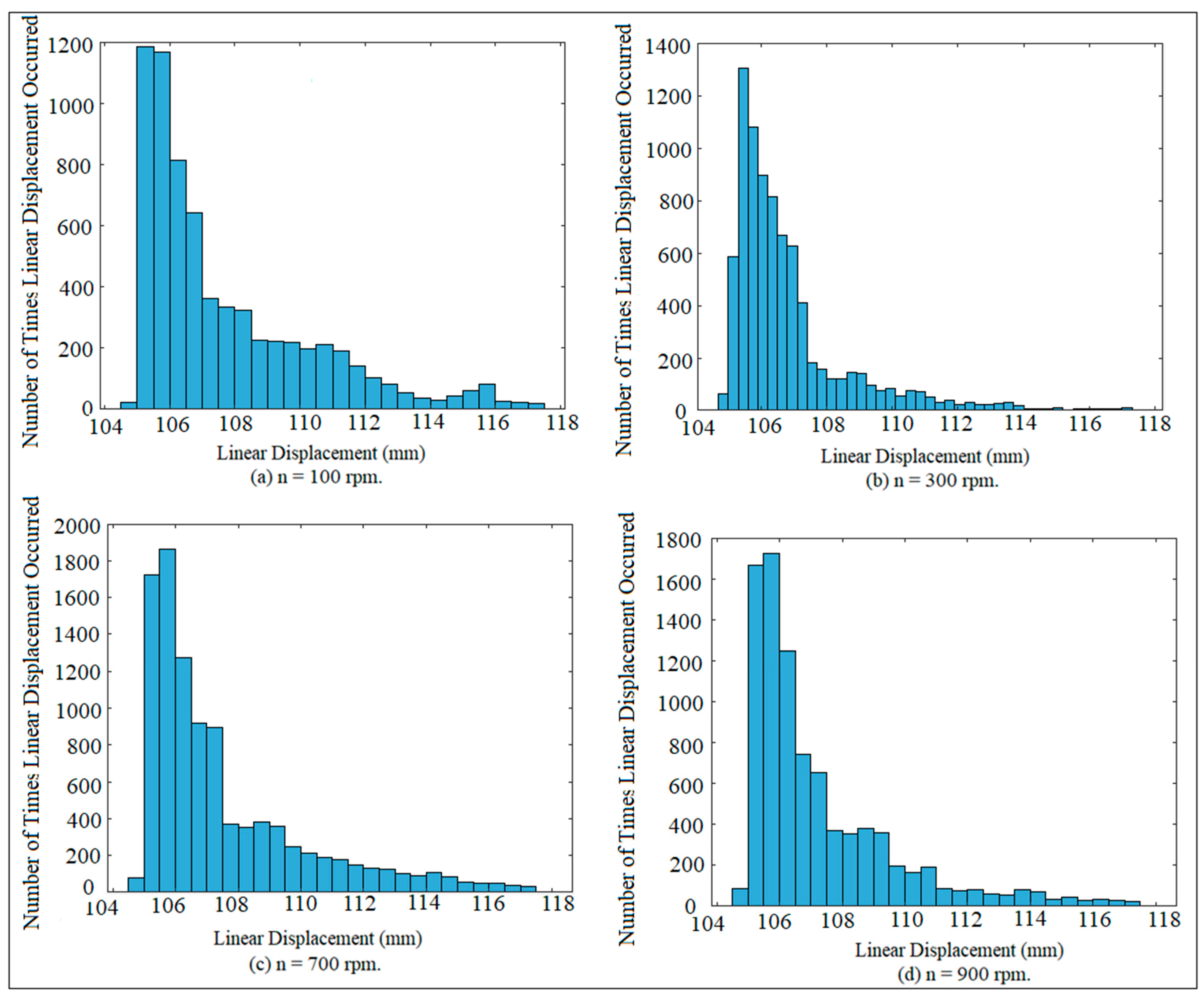
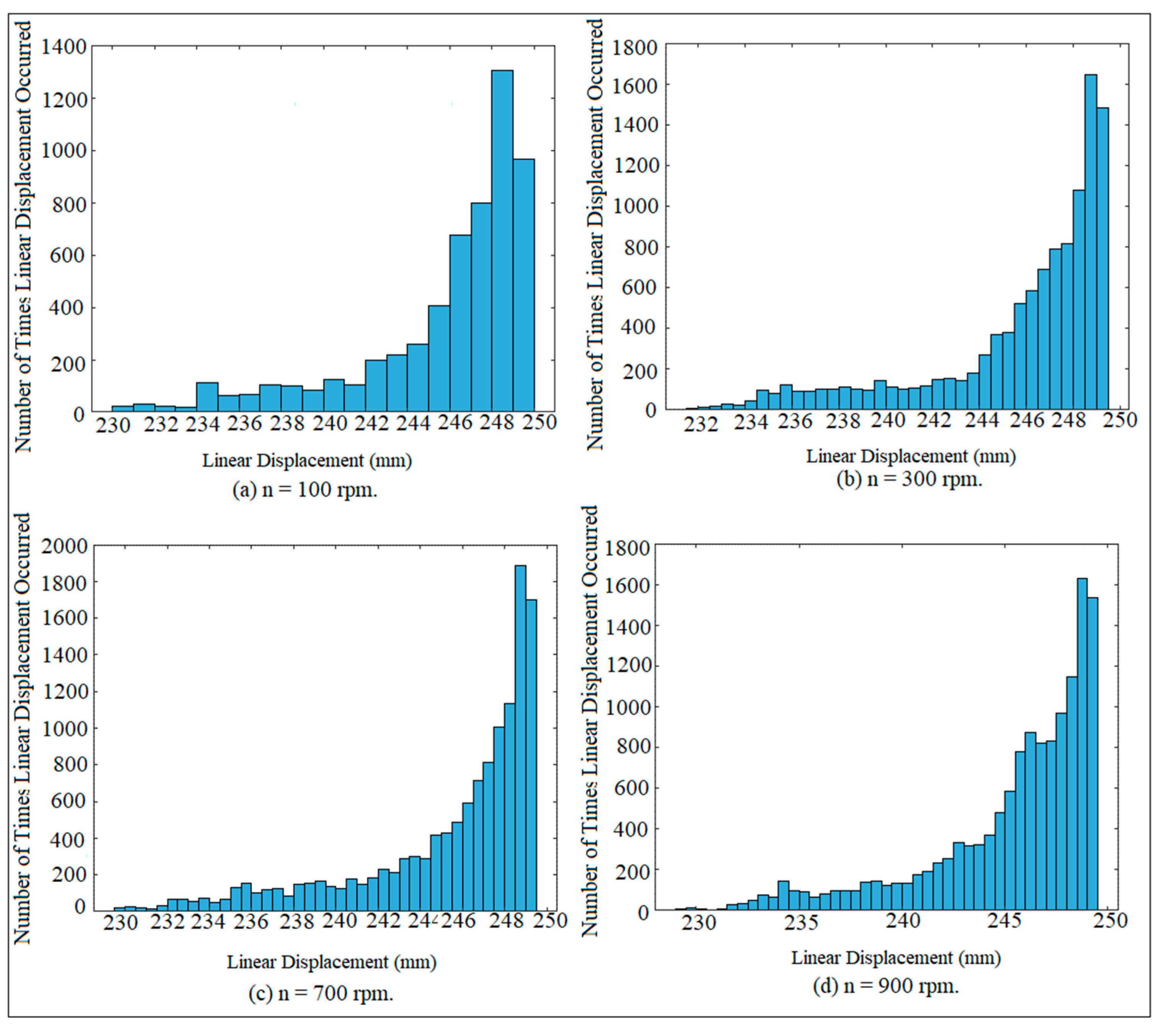
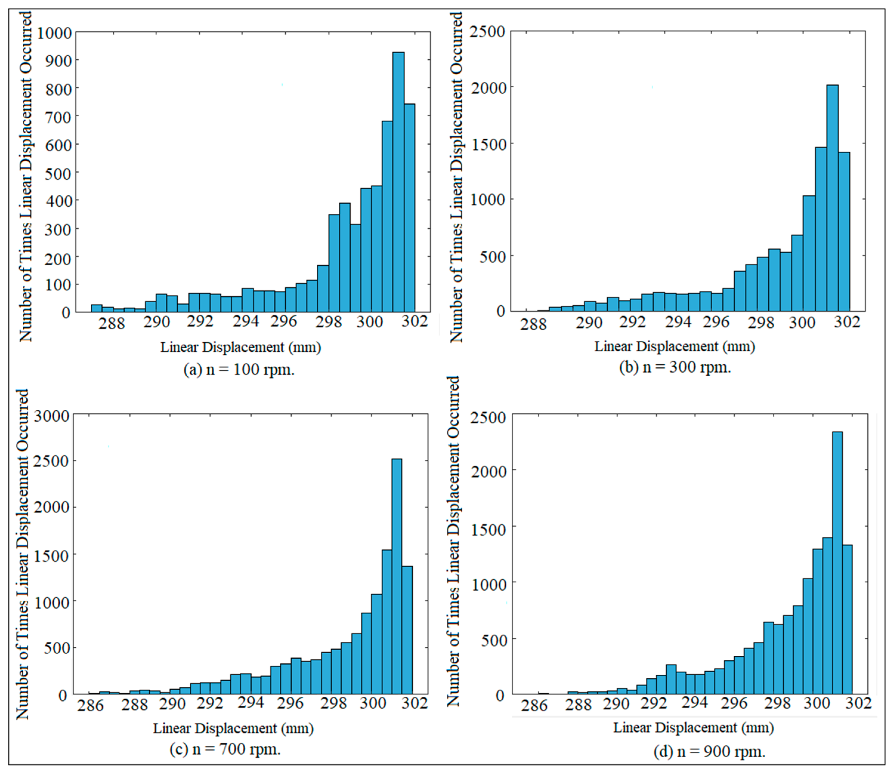
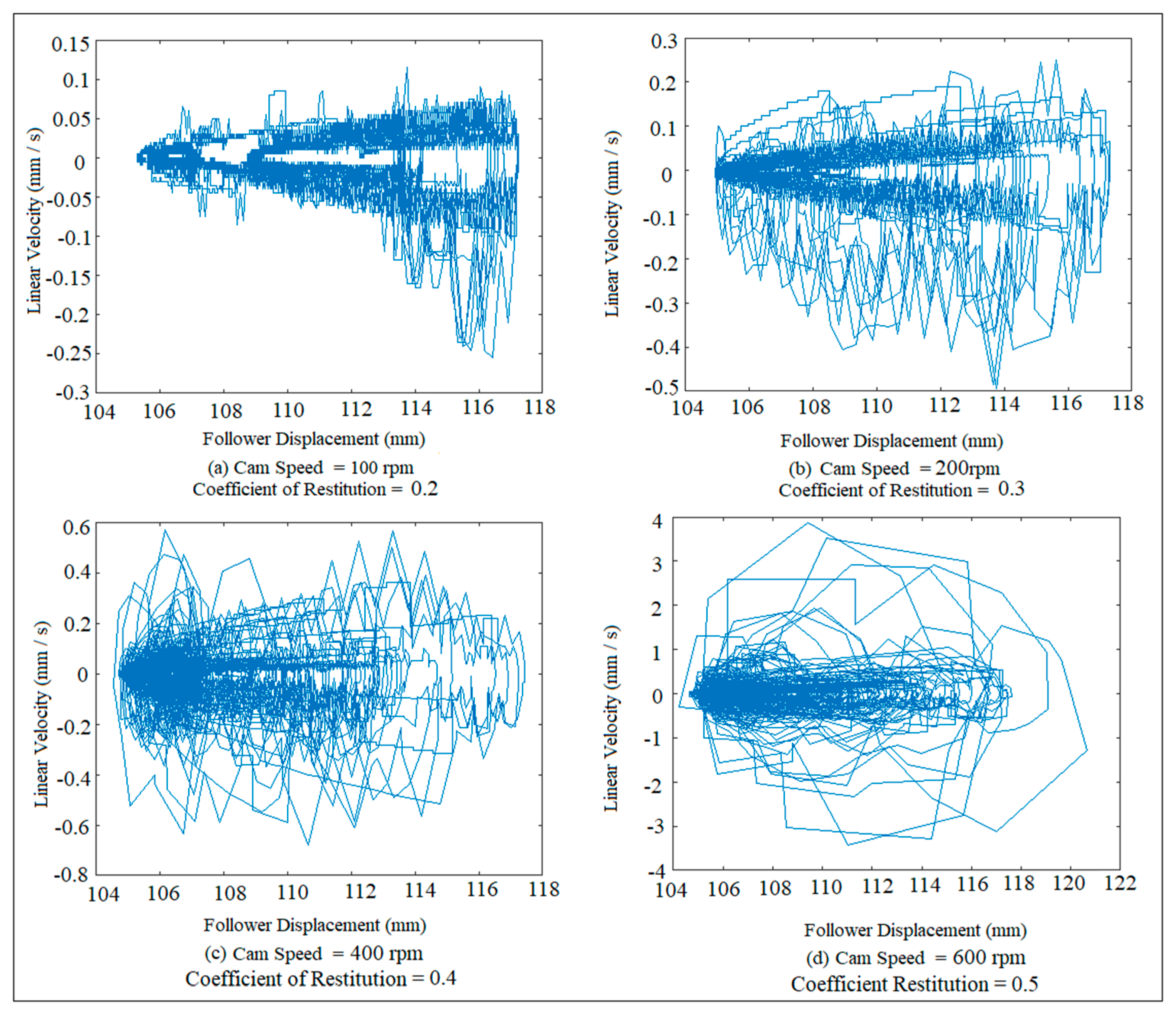
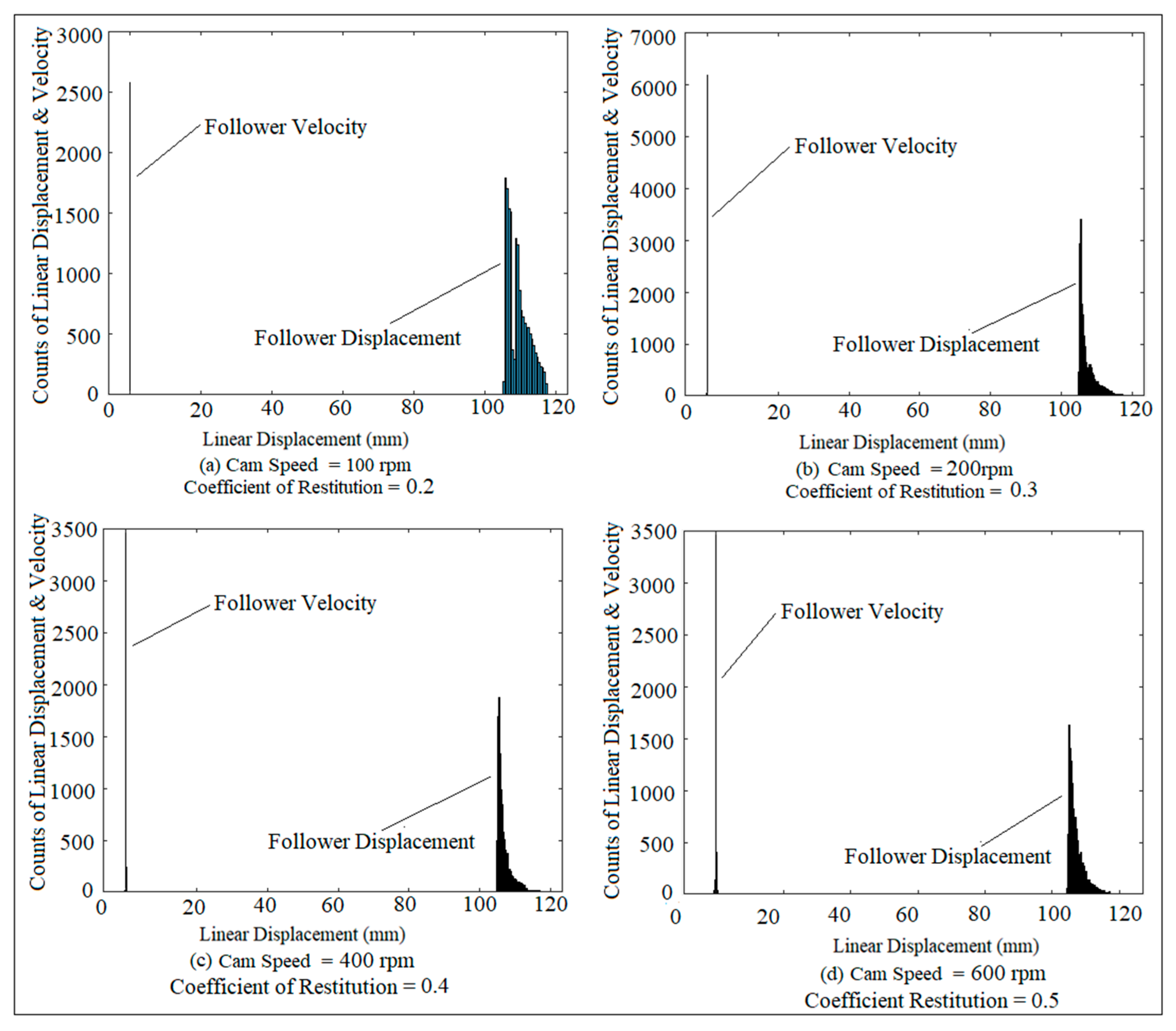
2. Chaotic Phenomenon Detection Using Linear Displacement

The SolidWorks program is used to find the solution of the dynamic motion [14] of the flat-faced follower, crank arm, and connecting rod. Follower displacement is used in the simulation by taking into consideration the effect of impact and friction. The guide distance (G.D.) 17 mm is selected at various speeds (n) of the cam (100 rpm, 300 rpm, 500 rpm, and 700 rpm). When the cam is spinning anticlockwise, it will force the flat-faced follower to move with three degrees of freedom (up–down, right–left, and rotation about z-axis) inside its guides; because of the clearance between the follower and the guides, chaotic motion will happen. There is a joint between the follower and the connecting rod and between the connecting rod and the crank arm. The motion of the follower will force the connecting rod and the crank arm to oscillate as a double pendulum. Both the cam and the crank arm are spinning about a fixed pivot. Figure 1 shows a planar mechanism with three moving links. All the dimensions are measured in mm. The SolidWorks program has three integrator solvers including GSTIFF, SI2-GSTIFF, and WSTIFF, which GSTIFF is used in the simulation. The maximum iteration is 25, while the initial integrator step size is 0.0001. The minimum integrator step size is 0.0000001, while maximum integrator step size is 0.001. The simulation parameters are the sliding contact velocity, kinetic coefficient of friction, contact body stiffness, exponent, maximum damping, and penetration. The symmetry and asymmetry of the chaotic phenomenon is investigated in which this phenomenon has been produced by the simulation artifacts based on the point linear displacement of the crank arm and connecting rod due to the movement of the follower. The points with the coordinates (X, Y, Z) in millimeters (−447.54, 9.47, −5), (−394.23, 13.73, −5), and (−40.38, −0.2, 0) which have been chosen on the crank arm, connecting rod, and flat-faced follower, respectively, are assigned in the SolidWorks program. Figure 2 shows the statistical diagram for the peak of point linear displacement for the follower. The systems with cam speeds (n) of 100 rpm, 300 rpm, 700 rpm, and 900 rpm and a guide distance (G.D.) 17 mm are selected in the simulation. The statistical diagram of the follower movement shows how many times that the follower detaches from the cam at different heights of detachment. The detachment starts at a follower movement of 105 mm for a cam speed of 100 rpm and it occurs couple times, while the separation occurs a hundred times for cam speeds of 300 rpm, 700 rpm, and 900 rpm at the same follower movement of the follower. The separation between the cam and the follower happens 1800 times at a follower movement of 106 mm for whole cam speeds. The separation between the cam and the follower decreases with the increment in follower movement for whole cam speeds, while the detachment completely disappears at a cam speed of 300 rpm after a follower movement of 114 mm.

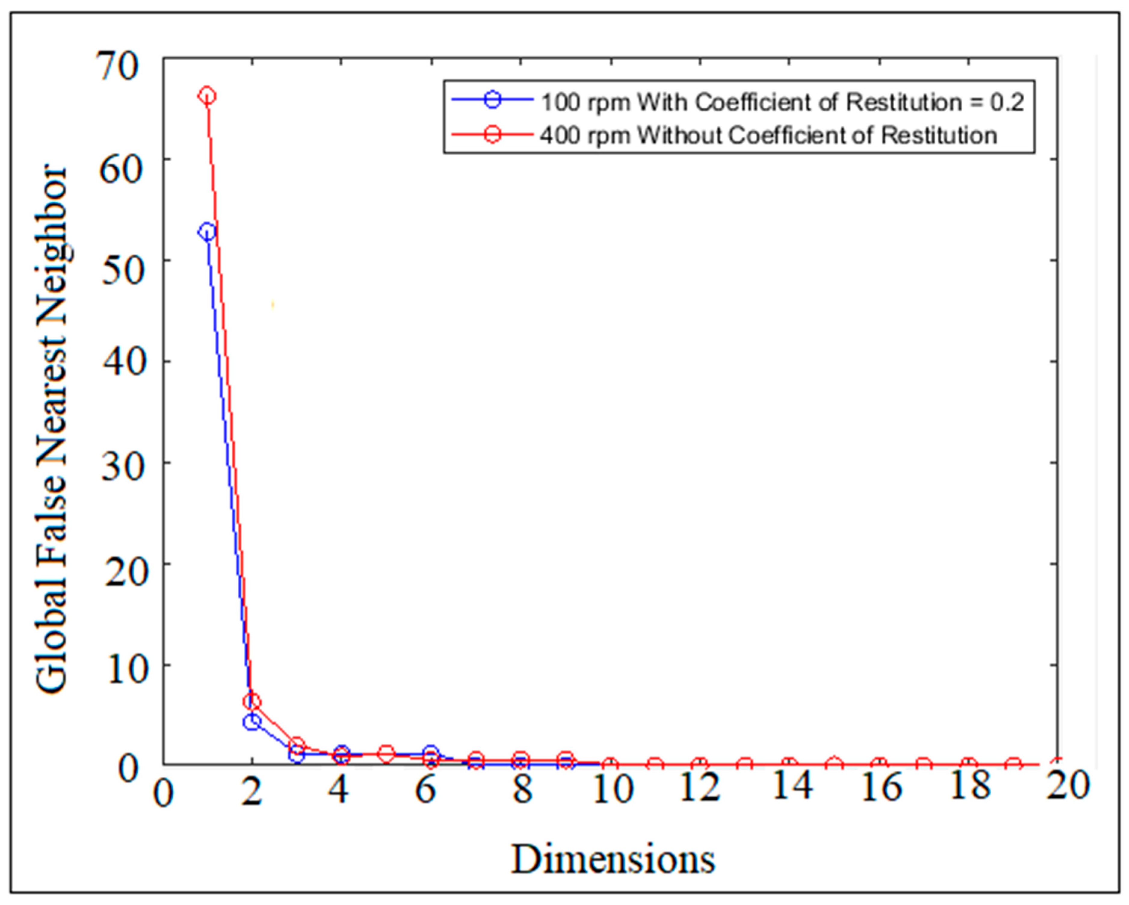
3. Global Dimensions of Chaotic Level

Global dimensions represent an algorithm which determines the global number of coordinates (d_E) of a space data factor of point linear displacement with the component [s(n), s(n + T), …, s(n + (d_E − 1)T)] while the method of false nearest neighbors is used. s(n) represents a format of a single column of the data set of the point linear displacement. The general dimension (d_E) is projected on the x-axis in which it is necessary for unfolding the data of the linear displacement against time. The exponential function of the global false nearest neighbor trend is decreased with the increase in the embedding dimensions at different cam speeds. A higher value of the time delay produces a trend of the global false nearest neighbors moving further away from the intersection with the x-axis of the embedding dimensions, while a smaller value of the time delay produces a trend of the global false neighbors intersecting with the x-axis of the embedding dimensions. Figure 3 shows the global embedding dimensions of a cam speed of n = 100 rpm at a coefficient of restitution of 0.2, and a cam speed of n = 400 rpm without the use of a coefficient of restitution. The value of the time delay is three for a cam speed of 400 rpm and one for a cam speed of 100 rpm. Fewer samples of point linear displacement are processed, while there are a number of samples to skip at the beginning of the data of the point linear displacement before evaluating the global false nearest neighbors. The minimum dimension is the smallest dimension in which the algorithm will test the unfolding of the original (ASCII) data of the point linear displacement using time delay coordinates. The default is one. The maximum dimension is the largest dimension in which the algorithm will investigate the false neighbor in the data of point linear displacement. The default is 15. The value of the time delay is too small when the global embedding dimension (d_E) is underestimated, while d_E is overestimated when the value of the time delay is too large. The decorrelation time is set at 10 times the value of the time delay from the average mutual information (AMI) as a default. The maximum neighbors, Tolerance 1, group factor, and Tolerance 2 are 400, 17.1, 20, and 1.81, respectively.

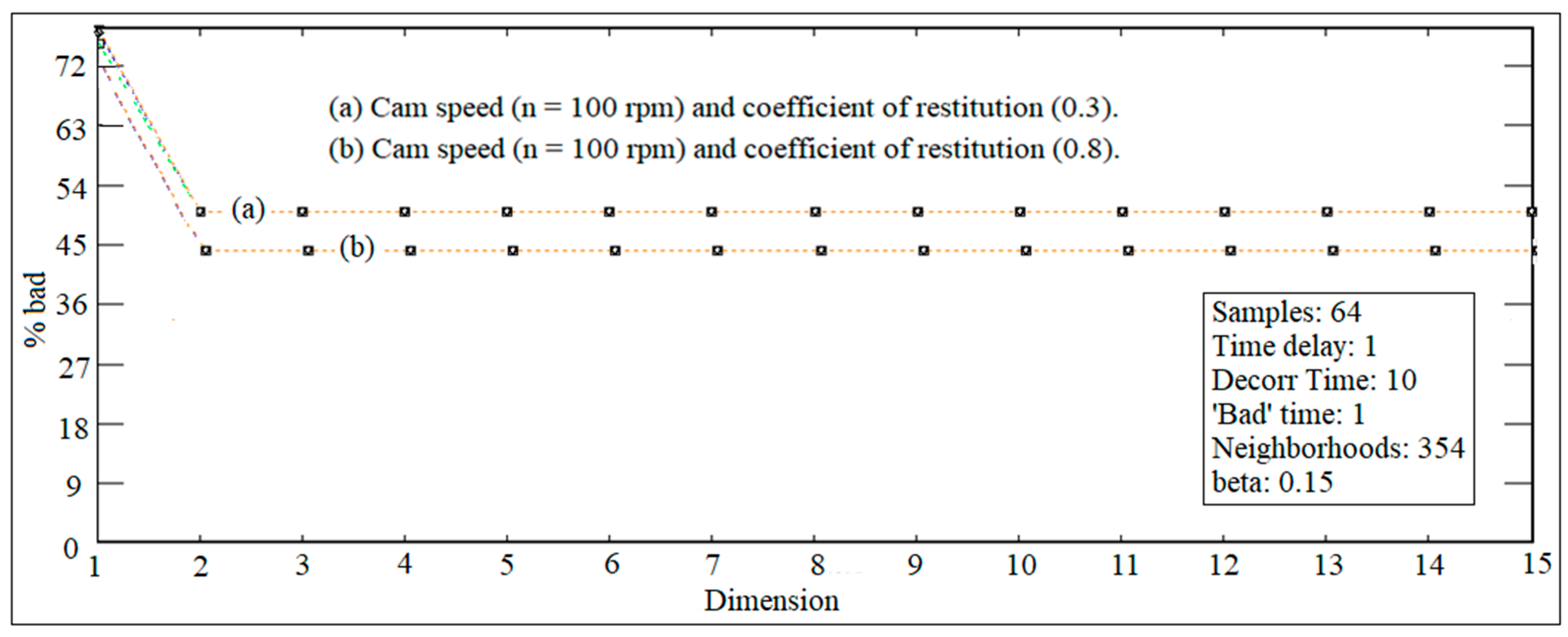
4. Local Dimensions of Chaotic Level

The local dimensions algorithm determines the number of active dynamical degrees of freedom (d_L) in the data set of point linear displacement based on the integer values of the time delay and embedding dimensions. The value of the time delay is an integer which represents the number of time units between the two samples of the point linear displacement. The method of average mutual information is used to find the value of the time delay. The value of the local embedding dimension (d_L) should be smaller than or equal to the value of the general dimension (d_E) and both are integers because globally the orbits of the system are twisted in the coordinate system constructed by the data of point linear displacement and its time delay. This dynamics tool converts the American Standard code for information and interchange (ASCII) file of point linear displacement to a simplified computational singular perturbation (CSP) format. The local and global dimensions are used to distinguish the difference between a low and high dimension of the chaos. The dynamic system has a low dimensional chaos when the embedding dimension is smaller than or equal to three [15], while the dynamic system has a high dimensional chaos when the embedding dimension is greater than three [16]. There is no formal definition between low dimensional chaos and high dimensional chaos. High dimensional chaos has been known as hyperchaos and it is characterized by more than one positive Lyapunov exponent parameter value, while low dimensional chaos is characterized by one positive Lyapunov exponent parameter value. The vertical axis is the percentage of bad predictions averaged over the number of starting locations selected by the user. The horizontal axis is the dimension of the model built in the algorithm. Figure 4 shows the local dimension histograms when the percentage of bad predictions for the date of point linear displacement becomes independent of the dimension and of the number of neighbors at (d_L = 2, and 2) to be the correct local in the dynamical dimension of the planar mechanism at a bad prediction of 49.5%, and 44%. Four evaluations of predictive capability in each of the dimensions for a default choice of 20, 40, 60, and 80 neighbors are used in the model building. The size criterion (beta = 0.15) with the number of neighborhoods as 3000 is selected. Fewer samples of point linear displacement are processed, while there are a number of samples to skip at the beginning of the data of the point linear displacement before evaluating the global false nearest neighbors. The value of the global dimension is reduced to be greater than or equal to d_E but the default is 15, while the decorrelation time is set at 10 times the value of the time delay from average mutual information (AMI) as a default. Time lag is the value inherited from the AMI. Bad time predicts a time default to the time lag from the AMI and this sets the time at which the quality of the predictions are evaluated by the algorithm. A large value of the number of neighborhoods is reasonable, which examines the quality of the predictions and will be an average over this quantity. The smaller the quantity, the faster the computation and the larger the root mean square (RMS) fluctuation about a reported mean. The group factor is a technical parameter used in the multidimensional search routine within the algorithm. The size criterion (beta) calculates how far apart as a fraction of the linear displacement attractor size points need to move to declare a bad prediction capability. The default is 0.1 but this value can be increased as far as 0.35 within the limits of accuracy for this algorithm. The exponential trend of local embedding dimensions measures the level of chaos, since the value of bad prediction decreases with the increase in the local embedding dimensions until the level of chaos settles down at a constant value. This constant value of the chaos level gives an indication of a low and high level of chaos.

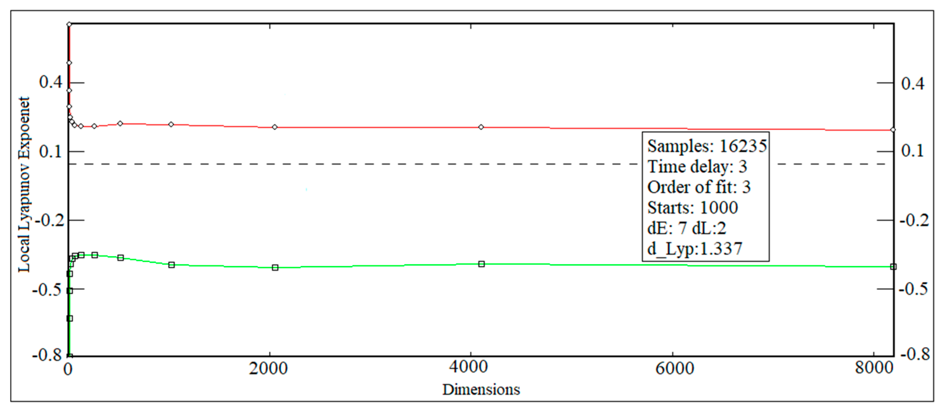
5. Chaotic Detection Using Local Lyapunov Exponent

The local Lyapunov exponent with and without a coefficient of restitution is used to detect the periodic and non-periodic motion of the point linear displacement attractor for the follower, connecting rod, and crank arm. The higher the value of Lyapunov exponent parameter, the more non-periodic the motion and chaos. When the value of the Lyapunov exponent parameter is positive, this means that there is an asymmetric rhythm in the attractor of follower displacement. A negative Lyapunov exponent parameter indicates a symmetric rhythm of the periodic motion. The Lyapunov exponent is quantified using the MATLAB code of the Wolf algorithm [17]. Equations (1) and (2) are used to build the Wolf algorithm code of the dynamic tool [18,19].

$$\mathrm{d}\left(\mathrm{t}\right)=\mathrm{D}{\mathrm{e}}^{\mathsf{\lambda }\mathrm{t}}$$

(1)

$$\mathrm{y}\left(\mathrm{i}\right)=\frac{1}{\Delta \mathrm{t}}[\mathrm{l}\mathrm{n}{\mathrm{d}}_{\mathrm{j}}(\mathrm{i})]$$

(2)

As stated earlier, a local embedding dimension smaller than or equal to three means that the dynamic system has a low level of chaos, while a dynamic system has a high level of chaos when the local embedding dimension is greater than three. In this paper, the local embedding dimension is smaller than three, which means that the mentioned planar mechanism has a low level of chaos. The Wolf algorithm is used since our mentioned dynamical system has a low level of chaos. The embedding dimension should be greater or equal to d_E as determined from the global false neighbors code algorithm, while the local dimension should be d_L as determined from the local false neighbors code algorithm. Fewer numbers of samples of point linear displacement are processed, while there are a number of samples to skip at the beginning of the data of the point linear displacement before evaluating the global false nearest neighbors. Time lag is the value inherited from the AMI. The correlation time is set to the time delay from the AMI. The number of starts of places on the point linear displacement attractor during the evaluation of the Lyapunov exponent in which all of these starts is documented for each number of steps beyond the starting point. It is recommended to accept the default of 1750. The polynomial order to fit in state space coordinates is used by making a local fit to neighborhood-to-neighborhood predictors. The linear term is used to determine the local Jacobian matrix in the quantification of the Lyapunov exponent. The default is cubic three. Moreover, the index factor is taken into account as a technical aspect of the search for neighbors in multidimensional space. The multi sampling time is evaluated in setting units for the computation of the Lyapunov exponent. It is recommended to accept the default of one. The power of length two is selected to be the total length from each point on the linear displacement attractor in which the algorithm evaluate the products of Jacobian matrices and the Lyapunov exponent. It is recommended to accept the maximum of 1024. True exponents have the same magnitude forward and backward in time simply by changing the sign. The default direction is forward. Figure 5 shows the local Lyapunov exponent of the follower movement against the global embedding dimensions at a cam speed 1800 rpm and a guide distance of 17 mm. The number of samples (16,235) of point linear displacement is selected to increase the precision of the value of the Lyapunov exponent at their respective equilibrium point. When the simulation time is increased, this leads to a settling down in the value of the Lyapunov exponent. The value of the Lyapunov exponent is positive, which means that the planar mechanism is in chaotic motion.

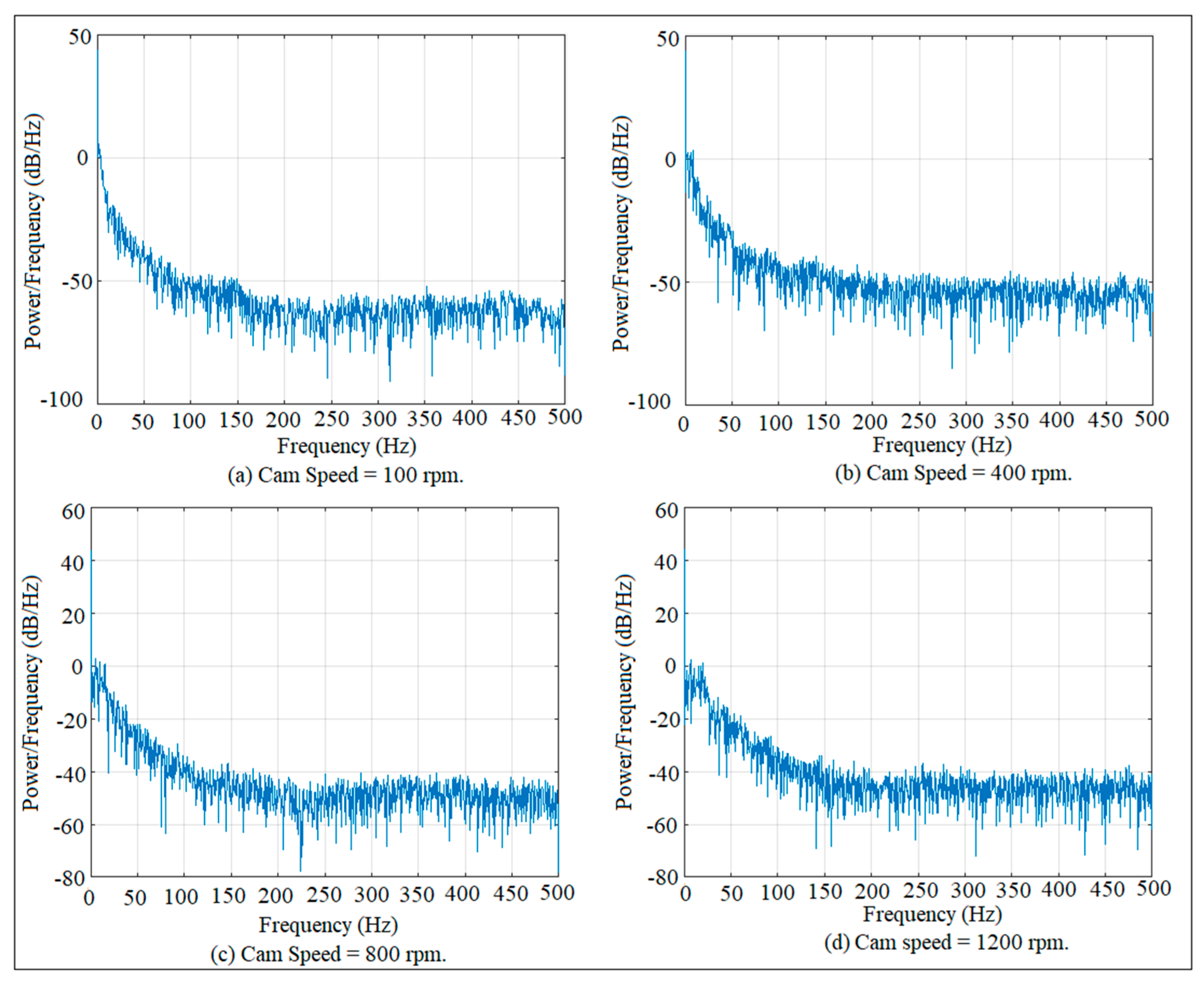
6. Fast Fourier Transform (FFT)

Fast Fourier transform of the power spectrum analysis technique is used to check the chaos level based on the signal-to-noise ratio factor (SNR) and the peak of the dominant frequency in the FFT diagram. The FFT diagram has been made based on the peak amplitude of the FFT function the time frequency value until the function of FFT settles down. The x-axis represents the time frequency (in mHz), while the y-axis reflects the peak amplitude of the FFT function (in mm). The value of the SNR factor decreased from a positive to a negative sign, which gives an indication of the chaos motion. Figure 6 shows how the peak amplitude of the FFT function is started appearing with the increasing of cam speeds at a guide distance of 17 mm until the function of FFT settles down at 700 samples of point linear displacement of the follower at the point of contact with the cam. Moreover, the SNR factor value decreased with the increase in cam speeds. The level of chaos is low as shown in Figure 6a, while the chaos is at a high level as indicated in Figure 6d.

7. Results and Discussion

Figure 7 and Figure 8 show the mapping of point linear displacement at various speeds of the cam at G.D. = 17 mm for the crank arm and connecting rod. The dynamic motion of the crank arm and connecting rod is similar to the dynamic motion of the double pendulum. The crank arm represents the first segment of the pendulum, while the connecting rod reflects the second segment of the pendulum. The track of the oscillation motion of the crank arm and connecting rod is irregular, which gives an indication of the non-periodic motion and chaos. The chaos of the oscillation motion of the crank arm is incremented with the increment in cam speeds. The track path of the oscillation motion of the connecting rod is smaller than the track path of the oscillation motion of the crank arm. The track path of the oscillation motion of the crank arm and connecting rod is non-periodic as shown in Figure 7a,b and Figure 8a,b, while the chaos motion of the oscillation motion of the crank arm and connecting rod is indicated in Figure 7c,d and Figure 8c,d. The time frequency of the oscillation motion of the connecting rod is smaller than the time frequency of the crank arm. The time frequency is irregular with the increment in cam speeds and its irregularity becomes more chaotic at a high speed of the cam. The motion of the crank arm and connecting rod is asymmetric based on the irregular track of the oscillation motion without the use of a coefficient of restitution, since there is no contact and impact does not happen on either the crank arm or the connecting rod. Figure 9 and Figure 10 show the histogram mapping of the connecting rod and crank arm at different cam speeds, respectively. The oscillation motion of the connecting rod is regular and it does not repeat itself frequently until the displacement reaches 234 mm as shown in Figure 9a,b, while it repeats a small amount as shown in Figure 9c. The oscillation motion of the connecting rod does not repeat itself at all at the displacement of 230 mm as shown in Figure 9d. The oscillation motion of the crank arm does not repeat itself until the displacement reaches 289 mm as indicated in Figure 10b,d, while the oscillation motion also does not repeat itself at the displacement of 287 mm, as shown in Figure 10d. The maximum counts of the oscillation motion are 950, 2000, 2500, and 2300 at the displacement of 301 mm as illustrated in Figure 10a–d.

Table 1. Local Lyapunov exponent against cam speeds for different guide distances.

Cam Speeds	700 rpm	900 rpm	1200 rpm	1500 rpm	1800 rpm	2000 rpm
Guide Distance = 17 mm	1.701	1.386	1.392	1.912	1.337	1.432
Guide Distance = 19 mm	1.710	1.661	1.513	1.308	1.368	1.652

shows the local Lyapunov exponent against cam speeds at different guide distances for the follower. The value of the local Lyapunov exponent is varied sinusoidal with the increasing of cam speeds while the value of the Lyapunov exponent is incremented with the increment in guide distances. The system with a cam speed of 1500 rpm and a guide distance of 17 mm is at a high level of chaotic motion, while the system with a cam speed of 1500 rpm and a guide distance of 19 mm is at a low level of chaotic motion. The chaotic level is the same for the systems with cam speeds (700 rpm) and guide distances (17 mm and 19 mm).

Figure 11 and Figure 12 show the trend of point linear displacement for the follower against time at different cam speeds and different coefficients of restitution. There is no effect of the coefficient of restitution on the point linear displacement for the follower. The frequency response of the dwell period is decreased with the increment in time and with the increment in cam speeds. The point linear displacement of the follower is symmetric against time at different values of the coefficients of restitution. There is no symmetry in the dwell period of time at different cam speeds.

Figure 13 shows the trend of global false nearest neighbors and when this trend approaches zero, which extracts the value of the embedding dimension for the crank arm at a cam speed of n = 100 rpm and a G.D. = 17 mm. Figure 14 shows the trend of the average mutual information, in which the minimum value in this trend gives an indication of the time delay for the crank arm at a cam speed of n = 100 rpm and a G.D. = 17 mm.

Figure 15 shows the Poincaré map of the follower displacement at different cam speeds and different coefficients of restitution. The Poincaré map is performed between the current point linear displacement and the next point linear displacement of the follower to catch the next periodicity of the follower movement. The chaos is at a low level as shown in Figure 15a, while the chaos is at a high level as illustrated in Figure 15d. The quasi-periodic motion of the follower movement is shown in Figure 15a,b, while the non-periodic motion is shown in Figure 15c. The chaotic motion of the follower is shown in Figure 15d. The Poincaré map gives an indication that the level of chaos is increased with the increment in cam speeds and with the increment in the coefficients of restitution. The black dots being stationed around the area inside the Poincaré diagram gives an indication of non-periodic motion and chaos, while the Poincaré diagram gives an indication of quasi-periodic motion when the black dots are separated from each other inside the Poincaré map.

Figure 16 shows the time history of the point linear displacement of the follower at different cam speeds and different coefficients of restitution. Figure 16 is related to Figure 15 since there are three sets of the periodicity of the follower displacement as mentioned in Figure 16a,c,f, while there are two sets of the periodicity of the follower movement as depicted in Figure 16b,d. There is just one set of the periodicity of the follower movement as shown in Figure 16e.

Figure 17 shows the phase-plane diagram of the point linear displacement of the follower at different cam speeds and different coefficients of restitution. The point linear displacement of the follower is varied (follower velocity) with the increment in cam speeds. The cross linking of the follower movement attractor is increased with the increment in the time simulation in which the chaotic motion is shown in Figure 17c,d. The chaotic motion is in low level and intangible with the increment in the coefficients of restitution as shown in Figure 17a,b. The simulation time is increased based on the contact between the cam and the follower and between the follower and its guides without the effect of the coefficient of restitution. Figure 18 shows the histogram of phase-plane mapping of the follower displacement at different cam speeds and different coefficients of restitution. The line at the left hand side represents the follower velocity, while the counts at the right hand side reflect the follower displacement. The value of the gradient of the follower displacement is tiny which appears like a line around zero compared with the large scale of the follower displacement. The follower velocity is increased with the increasing of cam speeds and with the increase in the coefficients of restitution. The separation between the cam and the follower happened 1800, 3500, 2000, and 1600 times, as indicated in Figure 18a–d after the follower displacement became 100 mm; and the counts of the separation occurring between the cam and the follower decreased with the increase in cam speeds and with the increase in the coefficients of restitution until they reached zero before the follower displacement became 120 mm.

Figure 19 shows the fast Fourier transform mapping of the flat-faced follower at different cam speeds and different coefficients of restitution for the guide distance of 17 mm using the power spectrum analysis technique. The chaotic level of this planar mechanism is increased with the increase in cam speeds and with the increase in the coefficients of restitution based on the SNR factor and the appearance of the amplitude of the peak of the FFT function. Figure 20 shows the mapping of the FFT function at different cam speeds at the guide distance of 19 mm. As stated above, the SNR factor value and the appearance of the amplitude of the peak of the FFT function play an important role in the detection of the level of chaos in the planar mechanism.

8. Conclusions

The finding of this paper is to detect the chaotic phenomenon for a crank arm and connecting rod due to the movement of the follower using fast Fourier transform, the largest Lyapunov exponent, and local and general embedding dimensions. The value of the local Lyapunov exponent is decreased with the increment in cam speeds in the presence of a coefficient of restitution. The value of the local Lyapunov exponent is increased with the increment in cam speeds without the use of a coefficient of restitution. There is no effect of the coefficient of restitution on the point linear displacement of the follower. The frequency response of the dwell period is decreased with the increment in time and with the increment in cam speeds. The point linear displacement of the follower is symmetric against time at different values of coefficients of restitution. There is no symmetry in the dwell period of time at different cam speeds.

References

1. Yan, H.S.; Tsai, W.J. A variable-speed approach for preventing cam-follower separation. J. Adv. Mech. Des. Syst. Manuf. 2008, 2, 12–23. [Google Scholar] [CrossRef]
2. Osorio, G.; di Bernardo, M.; Santini, S. Corner-impact bifurcations: A novel class of discontinuity-induced bifurcations in cam-follower systems. SIAM J. Appl. Dyn. Syst. 2008, 7, 18–38. [Google Scholar] [CrossRef]
3. Hongbin, Y.; Qingyuan, G.; Honghuan, Y.; Junquang, P. Analysis of the Influence of Machining Errors on the Dynamic Characteristics of the Dobby Modulator. J. Text. Eng. 2021, 67, 77–84. [Google Scholar]
4. Nguyen, T.T.N.; Duong, T.X.; Nguyen, V.-S. Design general Cam profiles based on finite element method. Appl. Sci. 2021, 11, 6052. [Google Scholar] [CrossRef]
5. Marghitu, D.B.; Zhao, J. Impact of a multiple pendulum with a non-linear contact force. Math. J. 2020, 8, 1202. [Google Scholar] [CrossRef]
6. De Groote, W.; Hoecke, S.V.; Crevecoeur, G. Physics-based neural network models for prediction of cam-follower dynamics beyond nominal operations. IEEE/ASME Trans. Mechatron. 2021, 27, 2345–2355. [Google Scholar] [CrossRef]
7. De Groote, W.; Kikken, E.; Hostens, E.; Van Hoecke, S.; Crevecoeur, G. Neural network augmented physics models for systems with partially unknown dynamics: Application to slider–crank mechanism. IEEE/ASME Trans. Mechatron. 2021, 27, 103–114. [Google Scholar] [CrossRef]
8. Cheng, Y.; Sun, Y.; Song, P.; Liu, L. Spatial-temporal motion control via composite cam-follower mechanisms. ACM Trans. Graph. 2021, 40, 1–15. [Google Scholar] [CrossRef]
9. Chang, X.; Pan, H.; Xu, J.; Wang, T. Study of Fault Identification of Clearance in Cam Mechanism. Appl. Sci. 2022, 12, 7420. [Google Scholar] [CrossRef]
10. Khajiyeva, L.A.; Kudaibergenov, A.K.; Abdraimova, G.A.; Sabirova, R.F. Modeling of Nonlinear Dynamics of Planar Mechanisms with Elastic and Flexible Pre-Stressed Elements; Advances in Mechanism Design III: Proceedings of TMM 2020 13; Springer: Cham, Switzerland, 2021; pp. 94–103. [Google Scholar] [CrossRef]
11. Jiang, S.; Chen, X. Test study and nonlinear dynamic analysis of planar multi-link mechanism with compound clearances. Eur. J. Mech. A/Solids 2021, 88, 104260. [Google Scholar] [CrossRef]
12. Alzate, R.; Piiroinen, P.T.; di Bernardo, M. From complete to incomplete chattering: A novel rout to chaos in impacting cam-follower systems. Appl. Sci. 2012, 22, 1250102. [Google Scholar] [CrossRef]
13. Wangqun, D.; Haibo, F.; Jianjun, W.; Yongfeng, Y. Effect of surface morphology on dynamic characteristics of cam-follower oblique impact system. J. Shock Vib. 2019, 2019, 3956169. [Google Scholar]
14. Planchard, D. SolidWorks 2016 Reference Guide: A Comprehensive Reference Guide with over 250 Standalone Tutorials; Sdc Publications: Mission, KS, USA, 2015. [Google Scholar]
15. Qiau, M.; Liang, Y.; Tavares, A.; Shi, X. Multilayer perceptron optimization for chaotic time series modeling. J. Entropy. 2023, 25, 973. [Google Scholar] [CrossRef] [PubMed]
16. Ott, E.; Antonsen, T.M. Low dimensional behavior of large systems of globally coupled oscillators. Chaos Interdiscip. J. Nonlinear Sci. 2008, 18, 037113. [Google Scholar] [CrossRef] [PubMed]
17. Ispolatov, I.; Madhok, V.; Allende, S.; Doebeli, M. Chaos in high-dimensional dissipative dynamical systems. J. Sci. Rep. 2015, 5, 12506. [Google Scholar] [CrossRef] [PubMed]
18. Parlitz, U. Estimating Lyapunov exponents from time series. In Chaos Detection and Predictability; Skokos, C., Gottwald, G.A., Laskar, J., Eds.; Springer: Berlin/Heidelberg, Germany, 2016; pp. 1–34. [Google Scholar]
19. Terrier, P.; Fabienne, R. Maximum Lyapunov exponent revisited: Long-term attractor divergence of gait dynamics is highly sensitive to the noise structure of stride intervals. J. Gait Posture 2018, 66, 236–241. [Google Scholar] [CrossRef] [PubMed]
Figure 1. Planar mechanism with three moving links.
Symmetry 15 02148 g001
Figure 2. Histogram mapping of follower displacement for G.D. = 17 mm at various speeds of the cam.
Symmetry 15 02148 g002
Figure 3. Global embedding dimensions at different cam speeds and different coefficients of restitution.
Symmetry 15 02148 g003
Figure 4. Local embedding dimensions at different cam speed and different coefficients of restitution.
Symmetry 15 02148 g004
Figure 5. Local Lyapunov exponent against global embedding dimensions for a cam speed of 1800 rpm and a guide distance of 17 mm.
Symmetry 15 02148 g005
Figure 6. Fast Fourier transform mapping at different cam speeds for the guide distance of 17 mm.
Symmetry 15 02148 g006
Figure 7. Mapping of point linear displacement for the crank arm at different cam speeds.
Symmetry 15 02148 g007
Figure 8. Mapping of point linear displacement for connecting rod at different cam speeds.
Symmetry 15 02148 g008
Figure 9. Histogram mapping of connecting rod at various speeds of the cam.
Symmetry 15 02148 g009
Figure 10. Histogram mapping of the crank arm at various speeds of the cam.
Symmetry 15 02148 g010
Figure 11. Follower linear displacement against time at a cam speed of n = 100 rpm and different coefficients of restitution.
Symmetry 15 02148 g011
Figure 12. Follower linear displacement against time at a cam speed of n = 200 rpm and different coefficients of restitution.
Symmetry 15 02148 g012
Figure 13. Embedding dimensions for crank arm at (n = 100 rpm).
Symmetry 15 02148 g013
Figure 14. Time delay for crank arm at (n = 100 rpm).
Symmetry 15 02148 g014
Figure 15. Poincaré map of the follower point linear displacement at different cam speeds and different coefficients of restitution.
Symmetry 15 02148 g015
Figure 16. Time history of the follower point linear displacement at different cam speeds and different coefficients of restitution.
Symmetry 15 02148 g016
Figure 17. Phase-plane of the follower displacement at different cam speeds and different coefficients of restitution.
Symmetry 15 02148 g017
Figure 18. Histogram of phase-plane mapping for the linear displacement and velocity of the follower at different cam speeds and different coefficients of restitution.
Symmetry 15 02148 g018
Figure 19. Fast Fourier transform mapping at different cam speeds and different coefficients of restitution for the guide distance of 17 mm.
Symmetry 15 02148 g019
Figure 20. Fast Fourier transform mapping at different cam speeds for the guide distance of 19 mm.
Symmetry 15 02148 g020