On Instabilities Caused by Magnetic Background Fields

Abstract

We review instabilities that appear from the coupling of spin-one fields to a magnetic background in a non-Abelian theory. Such coupling results, due to asymptotic freedom in a negative quantum, contribute to the effective potential. In QCD, the Savvidy vacuum results. However, due to the tachyonic mode, such a state is not stable, and the question about the true ground state of QCD is still open. In the electroweak model, the corresponding instability is postponed to very large background fields and may be of relevance in the early universe, at best. We start with an introduction to the topic and display the necessary formulas and methods. Then, we consider the one-particle spectra of the fields in a magnetic background and the related Euler–Heisenberg Lagrangians. In addition, we discuss the potential instability connected with the anomalous moment of the electron. The main part is on the quantum correction to the energy in non-Abelian fields, including massive ones. Here, the focus is on so-called electroweak magnetism and the search for a classical solution of the field equations and their approximations by a lattice of flux tubes. Finally, we review approaches with non-homogeneous background fields and the background of an $A_0$-field.

1. Introduction

Quantum Field Theory (QFT) describes the Standard Model (SM), which is fundamental for our current understanding of the micro-world. Beyond, the SM is only a narrow part of a huge variety of models in QFT, ranging from a mathematically strict formulation, especially in the curved background, to applications in solid state theory. In addition, QFT has many intriguing features, ranging from anomalies (which partly result in new discoveries) to instabilities resulting mainly in phase transitions. In general, instabilities can be found in many areas of classical physics, even in seemingly simple systems such as Newtonian gravity where the Jeans instability may cause a gas cloud to collapse (distinct from electric charges which repel if of the same sign).

In the present paper, a special class of instabilities is reviewed. The focus is on phenomena in magnetic background fields. Thereby, these may be of electromagnetic or of color magnetic nature. Magnetic fields cannot do work or transmit energy to a system. This is distinct from electric fields which can do work, for example separating a virtual electron–positron pair until it receives energy exceeding the mass of the pair so that it becomes real. However, in dependence on the mutual orientation, the interaction with a magnetic field with the magnetic moment of a particle may lower the energy, and interesting things may happen.

The instabilities we are interested in have two sources. One is the interaction of a spin’s magnetic moment with a magnetic background field, and the other is the self-interaction of a field that may result in a negative quantum contribution to the energy. Hereby, under ‘magnetic’, we subsume electromagnetic and color-magnetic, i.e., Abelian and non-Abelian, fields. The most prominent examples of negative quantum energy are the Casimir effect and the Coleman–Weinberg mechanism.

To be more specific, we consider quantum fields in a magnetic background field. To a large extent, these fields are homogeneous. From the linearized equations for the quantum fields, a spectrum follows,

$$\begin{array}{c}\hfill E=\sqrt{m^2+p_z^2+eB(2n+1+2s_z)},\end{array}$$

(1)

where E is the energy of a mode, m is the mass, and $p_z$ is the momentum parallel to the background field B, while e is a coupling constant. The quantum number $n=0,1,2,\dots$ describes the Landau levels, and $s_z=-s,-s-1,\dots ,s$ is the spin projection.

The ground state, i.e., the state with the lowest energy, has obviously $p_z=0$, $n=0$, and $s_z=-s$. However, for $s>\frac{1}{2}$, and $m=p_z=0$, the energy may become imaginary. Taken without further thought, this looks like a disaster. If one takes the time evolution, ∼$exp(\pm iEt)$, the imaginary part causes an exponential blow-up. Taken more seriously, imaginary energy signals an instability of the system, and a wider look at it is necessary (and may reveal interesting features).

The other source of instabilities, the quantum contribution to the vacuum energy, is in the lowest, one-loop approximation, given by the determinant of the kernel of the linearized action. It can be represented in the form

$$\begin{array}{c}\hfill E_{vac}={(-1)}^{2s}\frac{({\left(2s\right)}^2-\frac{1}{3}){\left(eB\right)}^2}{16{\pi }^2}ln\frac{eB}{{\mu }^2},\end{array}$$

(2)

following [1], p. 268, who coined the name ‘Nielsen–Olesen formula’, for a field with spin s. Here, $\mu$ is an arbitrary constant resulting from the usual arbitrariness of renormalization. In (2), the contribution ${\left(2s\right)}^2$ results from the interaction with the spin, whereas the ‘$\frac{1}{3}$’ results from the orbital motion.

The quantum vacuum energy must be considered together with the classical energy in an effective potential,

$$\begin{array}{c}\hfill V_{eff}=\frac{B^2}{2}+E_{vac}.\end{array}$$

(3)

For QED ($s=\frac{1}{2}$), we have

$$\begin{array}{c}\hfill V_{eff}=\frac{B^2}{2}-\frac{{\left(eB\right)}^2}{24{\pi }^2}ln\frac{eB}{{\mu }^2},\end{array}$$

(4)

and for QCD ($s=1$), we have

$$\begin{array}{c}\hfill V_{eff}=\frac{B^2}{2}+\frac{11{\left(gB\right)}^2}{48{\pi }^2}ln\frac{gB}{{\mu }^2},\left(SU\left(2\right)\right),\end{array}$$

(5)

where e and g are the corresponding coupling constants. Sometimes, these relations are also discussed in terms of the permeability of the vacuum. In analogy to the known formula, $E=\frac{1}{2}BH$ for the electromagnetic energy in a medium and the relation $B=\mu H$ (in the usual notations of macroscopic ED), the energies (4) and (5) can be expressed in the form

$$\begin{array}{c}\hfill V_{eff}=\frac{1}{2}\mu B^2,\end{array}$$

(6)

where

$$\begin{array}{c}\hfill {\mu }_{QED}=1-\frac{e^2}{24{\pi }^2}ln\frac{eB}{{\mu }^2},{\mu }_{QCD}=1+\frac{11g^2}{48{\pi }^2}ln\frac{eB}{{\mu }^2}\end{array}$$

(7)

are the corresponding permeabilities. The opposite sign in ${\mu }_{QCD}$ and in (5), as compared with the electromagnetic case, is, of course, the sign of asymptotic freedom. As a result, for small B, $V_{eff}$, Equation (5), has a minimum below zero. Equivalently, one may speak with ${\mu }_{QCD}<1$ of diamagnetism.

These two kinds of instabilities are in the focus of the present review. We start with the basic formulas for the various fields in a magnetic background. Then, we review the necessary field theoretic tools and the Euler–Heisenberg Lagrangians. In the fourth section, we consider instabilities caused by the quantum corrections and classical instabilities that gave rise to the notion of ‘electroweak magnetism’.

Finally, a remark on finite temperature is necessary. The investigation of quantum systems at finite temperature is an important tool in field theory. On the one hand, one expects high temperature to restore a broken symmetry; on the other hand, many processes happen at high temperature, such as, for example, heavy ions collisions or processes in the early universe. However, in general, temperature tends to remove instabilities; hence, we restrict ourselves here to $T=0$. An exception is the last section, where we consider an $A_0$-background, which is interesting only at finite temperature.

On the technical side, we simplify notations as much as possible. We use units with $\hslash =c=1$ in most places and employ the summation convention without further note. Throughout the paper, $A_{\mu }$ is the potential of the quantum gauge field, and $B_{\mu }$ is the potential of the background field. In some places, vector notation is used, which relates to the corresponding spatial parts.

2. Fields in a Magnetic Background

We consider a homogeneous magnetic background field, directed along the z-axis. Its action on a charge is, in classical terms, the Lorentz force, which enforces the motion on a circle. In the quantum language, the problem can be reduced to a harmonic oscillator whose energy levels are the Landau levels.

2.1. Scalar Field

We start from a scalar field in a magnetic background. Its Lagrangian reads

$$\begin{array}{cc}\hfill {\mathcal{L}}_{sc}\left(\varphi \right)& ={\left(D_{\mu }\varphi \right)}^{\ast }\left(D_{\mu }\varphi \right)-m^2{\varphi }^{\ast }\varphi ,\hfill \end{array}$$

(8)

where

$$\begin{array}{cc}\hfill D_{\mu }& ={\partial }_{\mu }-ie{A}_{\mu }\hfill \end{array}$$

(9)

is the covariant derivative realizing the minimal coupling, and e is the electric charge. Frequently, for the coupling, a plus sign is used in QED. We prefer the minus sign to have the same sign as in the non-Abelian case below. The electromagnetic potential, $A_{\mu }$, is related to the field strength and to the commutator by

$$\begin{array}{cc}\hfill F_{\mu \nu }& ={\partial }_{\mu }{A}_{\nu }-{\partial }_{\nu }{A}_{\mu },[D_{\mu },D_{\nu }]=-ie{F}_{\mu \nu }.\hfill \end{array}$$

(10)

The relation to the non-relativistic notations is $A_{\mu }={(\frac{1}{c}\Phi ,\overrightarrow{A})}_{\mu }$, $F_{ij}=-{ϵ}^{ijk}{B}_k$, where $B_k$ is the three dimensional magnetic field strength, ${ϵ}^{ijk}$ is the anti symmetric tensor, and $\Phi$ is the scalar potential.

In the following, we will mostly work with a homogeneous magnetic field. As usual, it points in the z-direction, $B_k=B{\delta }_{k3}$, and the related potentials are

$${\overrightarrow{A}}^{\mathrm{sy}}=\frac{B}{2}\left(\begin{array}{c}-y\\ x\\ 0\end{array}\right),{\overrightarrow{A}}^{\mathrm{L}}=B\left(\begin{array}{c}0\\ x\\ 0\end{array}\right).$$

(11)

The first is in the symmetric gauge, and the second is in the Landau gauge. These are related by a gauge transform, ${\overrightarrow{A}}^{\mathrm{sy}}={\overrightarrow{A}}^{\mathrm{L}}-\frac{B}{2}\nabla xy$.

The equation of motion following from the quadratic part of Lagrangian (8) is the Klein–Gordon equation,

$$\begin{array}{c}\hfill (D^2+m^2)\varphi =0,\end{array}$$

(12)

and the second derivative can be expanded as

$$\begin{array}{cc}\hfill D^2& ={\partial }^2-2ie{A}_{\mu }{\partial }_{\mu }-e^2{A}^2,\hfill \end{array}$$

(13)

assuming ${\partial }_{\mu }{A}_{\mu }=0$.

At this place, a digression to quantum mechanics may be useful. In the Schrödinger equation,

$$\begin{array}{cc}\hfill i\hslash {\partial }_t\Psi & =\left(\frac{{\overrightarrow{\pi }}^2}{2m}+e\varphi \right)\Psi \hfill \end{array}$$

(14)

with ${\overrightarrow{\pi }}^2=p^2-\frac{{\mu }_{\mathrm{B}}}{\hslash }\overrightarrow{L}\overrightarrow{A}+\frac{e^2}{2m}{A}^2$, using the quantum mechanical momentum operator $\overrightarrow{p}=\frac{\hslash }{i}\nabla$, the orbital momentum operator $\overrightarrow{L}=\overrightarrow{r}\times \overrightarrow{p}$ (writing $A^{\mathrm{sy}}$ in the form ${\overrightarrow{A}}^{\mathrm{sy}}=\frac{B}{2}(\overrightarrow{B}\times \overrightarrow{r})$), and the Bohr magneton ${\mu }_{\mathrm{B}}=\frac{e\hslash }{2m}$, the magnetic field couples to the orbital momentum $\overrightarrow{L}$. Further, turning to a two-component wave function $\Psi =\left(\begin{array}{c}{\varphi }_1\\ {\varphi }_2\end{array}\right)$, we come to the Pauli equation,

$$\begin{array}{cc}\hfill i\hslash {\partial }_t\Phi & =\left(\frac{{\overrightarrow{p}}^2}{2m}-\frac{{\mu }_{\mathrm{B}}}{\hslash }(\overrightarrow{L}+g\overrightarrow{s})\overrightarrow{A}+e\varphi \right)\Phi ,\hfill \end{array}$$

(15)

where we have in addition the spin operator $\overrightarrow{s}=\frac{\hslash }{2}\overrightarrow{\sigma }$ with the Pauli matrices $\overrightarrow{\sigma }$. The factor g is the gyromagnetic ratio, which remains open in quantum mechanics.

The spectrum, following from the operator in (12) for a homogeneous magnetic field (11), is well known,

$$\begin{array}{cc}\hfill p_0& =\sqrt{p_z^2+eB(2n+1)},(n=0,1,\dots )\hfill \end{array}$$

(16)

where $p_0$ and $p_z$ are the eigenvalues of the corresponding momentum operators, and n enumerates the Landau levels. These energy levels are degenerated as being independent on a further quantum number. In the Landau gauge, we have translational invariance in the y-direction, and in the symmetric gauge, rotational invariance around the z-axis. The degeneracy factor is the number of flux units per unit area. The magnetic part of the spectrum is equally spaced, and it is the same as that of a quantum mechanical harmonic oscillator, since commutator (10) is a constant.

We mention also the spectrum for Pauli Equation (15)

$$\begin{array}{c}\hfill E=\frac{p_z^2}{2m}+\frac{{\mu }_B}{\hslash }B(2n+1+g{s}_z),\end{array}$$

(17)

which is nonrelativistic. Here, the spin projection $s_z$ enters.

2.2. Spinor Field

The Lagrangian reads

$$\begin{array}{cc}\hfill {\mathcal{L}}_{sp}& =\overline{\psi }(i{\gamma }^{\mu }{D}_{\mu }-m)\psi ,\hfill \end{array}$$

(18)

where $\psi$ is a Dirac spinor, and ${\gamma }^{\mu }$ are the gamma matrices obeying the anti-commutator relation

$$\begin{array}{c}\hfill {\gamma }^{\mu }{\gamma }^{\nu }+{\gamma }^{\nu }{\gamma }^{\mu }=2g^{\mu \nu }.\end{array}$$

(19)

The Dirac equation, following from (18),

$$\begin{array}{c}\hfill (i{\gamma }^{\mu }{D}_{\mu }-m)\psi =0,\end{array}$$

(20)

can be ‘squared’ by multiplying from left by $(i{\gamma }^{\mu }{D}_{\mu }+m)$,

$$\begin{array}{c}\hfill ({\left(i{\gamma }^{\mu }{D}_{\mu }\right)}^2-m^2)\psi =0,\end{array}$$

(21)

and using (19) and commutator (10), one arrives at

$$\begin{array}{c}\hfill (D^2-\frac{e\hslash }{2}{\sigma }^{\mu \nu }{F}_{\mu \nu }-m^2)\psi =0\end{array}$$

(22)

with the antisymmetric spin matrix ${\sigma }^{\mu \nu }=\frac{i}{2}({\gamma }^{\mu }{\gamma }^{\nu }-{\gamma }^{\nu }{\gamma }^{\mu })$. For the spatial components, we note

$${\sigma }^{ij}=-{ϵ}^{ijk}\left(\begin{array}{cc}0& -{\sigma }_k\\ {\sigma }_k& 0\end{array}\right)\equiv {ϵ}^{ijk}{S}_k,\overrightarrow{S}=\left(\begin{array}{cc}0& \overrightarrow{\sigma }\\ -\overrightarrow{\sigma }& 0\end{array}\right).$$

(23)

In a homogeneous background field, using (13), we arrive at

$$\begin{array}{c}\hfill ({\partial }^2+e(\overrightarrow{L}+g\overrightarrow{S})\overrightarrow{B}-{(e\overrightarrow{A})}^2)\psi =0.\end{array}$$

(24)

This way, the gyromagnetic ratio $g=2$ follows from the Dirac equation, with opposite spin projections for the upper and the lower components.

One may ask for generalizations of the Dirac equation, of which there are. The most general equation involving only the dimensions that appear in Equation (22) differs from this equation by adding a direct interaction with the spin operator in the form (it is the only covariant way in the given dimension)

$$\begin{array}{c}\hfill (i{\gamma }^{\mu }{D}_{\mu }-a_e\frac{e\hslash }{4}{\sigma }^{\mu \nu }{F}_{\mu \nu }-m)\psi =0,\end{array}$$

(25)

which, in a lowest approximation by ’squaring’ the equation, results in a change of the gyromagnetic ratio in Equation (24). It is usually formulated in terms of the anomaly factor,

$$\begin{array}{c}\hfill a_e=\frac{g-2}{2}\end{array}$$

(26)

in Equation (25). It was first calculated by [2], who found $a_e=\frac{\alpha }{2\pi }$ at the one loop level. Considering Equation (25) with a non-zero anomaly factor as a starting point results in a non-renormalizable theory. It is only higher loop corrections that may deliver an anomaly while not destroying renormalizability. This may be viewed in parallel to the Higgs mechanism, delivering a mass to gauge fields, where the direct introduction of a mass term would destroy gauge invariance.

In a homogeneous background field, the spectrum of the operator in Equation (25), which corresponds to (16), reads

$$\begin{array}{c}\hfill p_0=\sqrt{p_z^2+eB(2n+1+2(1+a_e)s)+m^2},\end{array}$$

(27)

where $s=\pm \frac{1}{2}$ is the spin projection. An interesting point is the case $n=0$, $s=-\frac{1}{2}$, where the coupling of the spin (without anomaly) to the background field just compensates for the energy of the lowest Landau level. The latter is conceptually the same as the zero-point energy of a harmonic oscillator. Including the anomaly, one observes an overcompensation, which will be discussed in Section 3.4. These energy levels are illustrated in Figure 1, left panel.

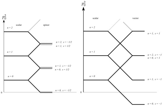
Figure 1. The lowest energy levels in a homogeneous magnetic field. The left panel shows the levels of a scalar field that are split by the spin interaction of the spinor field. An additional level splitting, which is due to the anomalous magnetic moment, is shown as dotted lines (and magnified). The right panel shows the levels of a scalar field that is split by the spin interaction of a vector field.

2.3. Abelian Vector Field

An Abelian vector field is basically the electromagnetic field, although it may also appear as one isospin component of other fields. It can be represented by a vector potential, $A_{\mu }$, and the field strength, $F_{\mu \nu }$, as in Equation (10). Its Lagrangian reads

$$\begin{array}{c}\hfill {\mathcal{L}}_{ED}\left(A_{\mu }\right)=-\frac{1}{4}{\left(F_{\mu \nu }\right)}^2=\frac{1}{2}{A}_{\mu }\left({\partial }^2{g}_{\mu \nu }-{\partial }_{\mu }{\partial }_{\nu }\right)A_{\nu },\end{array}$$

(28)

where total derivative terms were dropped. This Lagrangian is singular due to its gauge invariance, and one has to apply well-known procedures such as gauge fixing and Faddeev–Popov fields (usually not in ED). We do not enter here the details of this. A background field $B_{\mu }$ is introduced simply by ${\mathcal{L}}_{ED}\left(A_{\mu }\right)\to {\mathcal{L}}_{ED}(A_{\mu }+B_{\mu })$, and in the quadratic terms, there is no coupling to the background field.

2.4. Non-Abelian Vector Field

A non-Abelian vector field is a representation of a non-Abelian group such as SU(2) or SU(N). We restrict ourselves to the simplest case of SU(2) and represent here only the minimal information needed in the following. The vector potential $A_{\mu }^a$ has an additional index, $a=1,2,3$, belonging to the fundamental representation and, considering the QCD, can be called the color index. The field strength and the covariant derivative read

$$\begin{array}{c}\hfill F_{\mu \nu }^a={\partial }_{\mu }{A}_{\nu }^a-{\partial }_{\nu }{A}_{\mu }^a+g{ϵ}^{abc}{A}_{\mu }^b{A}_{\nu }^c,D_{\mu }^{ab}={\partial }_{\mu }{\delta }^{ab}+g{ϵ}^{acb}{A}_{\mu }^c,\end{array}$$

(29)

where ${ϵ}^{abc}$ is, again, the antisymmetric tensor. It is common to denote the coupling constant, or color charge, by g distinct from the electric charge e. The commutator is

$$\begin{array}{c}\hfill {[D_{\mu },D_{\nu }]}^{ab}=g{ϵ}^{acb}{F}_{\mu \nu }^a.\end{array}$$

(30)

The Lagrangian, in terms of the field strength, looks formally the same as before; however, from the commutator, we have more structures,

$$\begin{array}{c}\hfill {\mathcal{L}}_{SU\left(2\right)}\left(A\right)=-\frac{1}{4}{\left(F_{\mu \nu }^a\right)}^2={\mathcal{L}}_2+{\mathcal{L}}_3+{\mathcal{L}}_4,\end{array}$$

(31)

where

$$\begin{array}{c}\hfill {\mathcal{L}}_2=\frac{1}{2}{A}_{\mu }^a\left({\partial }^2{g}_{\mu \nu }-{\partial }_{\mu }{\partial }_{\nu }\right)A_{\mu }^a\end{array}$$

(32)

is the quadratic part and

$$\begin{array}{c}\hfill {\mathcal{L}}_3=-g{ϵ}^{abc}\left({\partial }_{\mu }{A}_{\nu }^a\right)A_{\mu }^b{A}_{\nu }^c,{\mathcal{L}}_4=-\frac{g^2}{2}(A_{\mu }^a{A}_{\mu }^a{A}_{\nu }^b{A}_{\nu }^b-A_{\mu }^a{A}_{\nu }^a{A}_{\mu }^b{A}_{\nu }^b)\end{array}$$

(33)

are the triple and quartic parts. These represent the self-interaction that appears in the non-Abelian case, distinct from the Abelian one.

A background field $B_{\mu }^a$ is added such as in the Abelian case, but the formulas become more involved. Keeping previous notations,

$$\begin{array}{c}\hfill {\mathcal{L}}_{SU\left(2\right)}(A+B)={\mathcal{L}}_{SU\left(2\right)}\left(B\right)+{\mathcal{L}}_1+{\mathcal{L}}_2+{\mathcal{L}}_3+{\mathcal{L}}_4,\end{array}$$

(34)

where now,

$$\begin{array}{cc}\hfill {\mathcal{L}}_2& =\frac{1}{2}{A}_{\mu }^a\left(D^2{g}_{\mu \nu }{\delta }^{ab}-D_{\nu }^{ac}{D}_{\mu }^{cb}-g{ϵ}^{acb}{B}_{\mu }^c\right)A_{\mu }^b,\hfill \\ \hfill {\mathcal{L}}_3& =-g{ϵ}^{abc}\left(D_{\mu }^{ad}{A}_{\nu }^d\right)A_{\mu }^b{A}_{\nu }^c,\hfill \end{array}$$

(35)

and ${\mathcal{L}}_4$ remains unchanged. Finally,

$$\begin{array}{c}\hfill {\mathcal{L}}_1=A_{\nu }^a{D}_{\mu }^{ab}{F}_{\mu \nu }^b\left(B\right)\end{array}$$

(36)

is the linear term, which vanishes, for instance, for a homogeneous, Abelian background field.

In the above formulas, the derivatives had been changed for the covariant ones in the background,

$$\begin{array}{c}\hfill D_{\mu }^{ab}={\partial }_{\mu }{\delta }^{ab}+g{ϵ}^{acb}{B}_{\mu }^b,{[D_{\mu },D_{\nu }]}^{ab}=g{ϵ}^{acb}{F}_{\mu \nu }^a\left(B\right).\end{array}$$

(37)

(we no longer use the definition from (29)). The additional term in ${\mathcal{L}}_2$ comes from ${\mathcal{L}}_3$ in (33), and we have to note the indices in the second term in parenthesis. Interchanging these results in a commutator term (which does not appear in the Abelian case), we arrive at

$$\begin{array}{cc}\hfill {\mathcal{L}}_2& =\frac{1}{2}{A}_{\mu }^a\left(D^2{g}_{\mu \nu }{\delta }^{ab}-D_{\mu }^{ac}{D}_{\nu }^{cb}-2g{ϵ}^{acb}{B}_{\mu }^c\right)A_{\mu }^b,\hfill \end{array}$$

(38)

which is the quadratic part of the Lagrangian in an arbitrary background field.

In the following, we will restrict ourselves to Abelian background fields,

$$\begin{array}{c}\hfill B_{\mu }^a=B_{\mu }{\delta }^{a3}.\end{array}$$

(39)

These point in one direction in the color space, and their field strength is similar to the Abelian case,

$$\begin{array}{c}\hfill F_{\mu \nu }^a\left(B\right)=F_{\mu \nu }{\delta }^{a3},F_{\mu \nu }={\partial }_{\mu }{B}_{\nu }-{\partial }_{\nu }{B}_{\mu }.\end{array}$$

(40)

In this case, it is useful to turn into the so-called ‘charged basis’ by a unitary transform,

$$\begin{array}{c}\hfill W_{\mu }=\frac{1}{\sqrt{2}}(A_{\mu }^1+i{A}_{\mu }^2),A_{\mu }=A_{\mu }^3.\end{array}$$

(41)

The potentials $A_{\mu }^a$ are real fields, $W_{\mu }$ is a complex field (there is also its complex conjugate, $W_{\mu }^{*}$), and the third component, $A_{\mu }$, remains real. The field $W_{\mu }$ can be interpreted as a color-charged vector field and $A_{\mu }$ as a color-neutral vector field. We mention that in SU(3), a similar transformation yields two neutral fields, $A_{\mu }^3$ and $A_{\mu }^8$, and three pairs of color-charged fields which, distinct from SU(2), already have their interpretation in the theory of strong interactions.

Rewriting the Lagrangian in terms of these fields, we arrive at

$$\begin{array}{cc}\hfill {\mathcal{L}}_2& =W_{\mu }^{*}\left(D^2{\delta }_{\mu \nu }-D_{\mu }{D}_{\nu }+2ig{B}_{\mu \nu }\right)W_{\nu }+\frac{1}{2}{A}_{\mu }\left({\partial }^2{\delta }_{\mu \nu }-{\partial }_{\mu }{\partial }_{\nu }\right)A_{\nu },\hfill \\ \hfill {\mathcal{L}}_3& =-ig(A_{\mu }{W}_{\mu \nu }^{*}{W}_{\nu }+A_{\mu }{W}_{\nu }^{*}{W}_{\mu \nu }-B_{\mu \nu }{W}_{\mu }^{*}{W}_{\nu }),\hfill \\ \hfill {\mathcal{L}}_4& =-g^2(A_{\mu }{A}_{\mu }{W}_{\nu }^{*}{W}_{\nu }-A_{\mu }{A}_{\nu }{W}_{\mu }^{*}{W}_{\nu }+W_{\mu }^{*}{W}_{\mu }{W}_{\nu }^{*}{W}_{\nu }-W_{\mu }^{*}{W}_{\nu }{W}_{\mu }^{*}{W}_{\nu }).\hfill \end{array}$$

(42)

Here, the covariant derivative is

$$\begin{array}{c}\hfill D_{\mu }={\partial }_{\mu }-ie{B}_{\mu },[D_{\mu },D_{\nu }]=-i{F}_{\mu \nu }\left(B\right),\end{array}$$

(43)

and we use the notations $A_{\mu \nu }={\partial }_{\mu }{A}_{\nu }-{\partial }_{\mu }{A}_{\nu }$ and $W_{\mu \nu }=D_{\mu }{W}_{\nu }-D_{\mu }{W}_{\nu }$ (only in this formula), and $F_{\mu \nu }$ is a constant antisymmetric tensor.

As a background field, we consider the $a=3$ component $A_{\mu }$. This is a so-called Abelian background field since its field strength is given by Equation (28), i.e., such as in ED. The reason behind this is that a field pointing in only one direction in color space has no quadratic contribution in its field strength (29), which vanishes due to the antisymmetry of the structure constant, the epsilon tensor in our case. Further, we take a homogeneous background as before. In such a background field, the spectrum of the operator in the quadratic part of the $W_{\mu }$ field, taking in addition $D^{\mu }{W}_{\mu }=0$ as gauge fixing, generalizing (16) and (27), reads

$$\begin{array}{c}\hfill p_0=\sqrt{p_z^2+gB(2n+1+2s_z)},\end{array}$$

(44)

where now the spin projection is $s_z=\pm 1$. Here, the interesting case is $n=0$, $s=-1$, where the interaction of the magnetic moment overcompensates for the lowest Landau level twice, and for a momentum $p_z<gB$, the one particle energy $p_0$ becomes imaginary. These energy levels are illustrated in Figure 1, right panel.

3. Vacuum Energy in Magnetic Background Fields—Euler–Heisenberg Lagrangian

In this section, we consider the most common effects appearing in one-loop approximation in magnetic background fields. We start with an introduction of the basic methods and advance to their application in several models.

3.1. Field Theoretic Methods

In this subsection, we consider a collection of some basic formulas of quantum field theory (QFT). Thereby, we use the Euclidean version and will keep the formulas as simple as possible. A field $\varphi$ is, for the beginning, a generic object in the sense of condensed notations, and summations/integrations are assumed. The basic object is the generating functional Z,

$$\begin{array}{c}\hfill Z\left(J\right)=\int D\varphi e^{S+J\varphi },S=\int dx\mathcal{L},\end{array}$$

(45)

defined by a functional integral, in terms of an action S and the corresponding Lagrangian $\mathcal{L}$. A possible normalization factor in front of the functional integral remains indeterminate. The derivatives of Z with respect to the source J are the Green’s function of the theory defined by $\mathcal{L}$. As well known, all these formulas are classical ones (no operators), but with the functional integral, we obtain the corresponding expressions of a QFT.

The functional integral is, of course, a formal construct. We will give it a meaning in perturbation theory. For this, we define the free part of the action from terms at the quadratic in the field and divide the action,

$$\begin{array}{c}\hfill S=S_0+S_{int},\end{array}$$

(46)

into free and interaction parts. In the free part, we have a quadratic term in the field,

$$\begin{array}{c}\hfill S_2=\frac{1}{2}\int dx\varphi K\varphi ,\end{array}$$

(47)

where K is a kernel. In momentum representation, and without a background field, i.e., in the simplest case, it takes the form

$$\begin{array}{c}\hfill K=-p^2-m^2,\end{array}$$

(48)

where $p^2=p_{\mu }{p}^{\mu }$ is the squared (Euclidean) momentum. The minus sign is included here for convenience.

The transition to the perturbation theory can be performed using the following construction,

$$\begin{array}{c}\hfill Z\left(J\right)=e^{S_{int}\left(\frac{\delta }{\delta J}\right)}\int D\varphi e^{S_2+\varphi J}.\end{array}$$

(49)

The remaining integral is an infinite dimensional generalization of a Gaussian integral and can be calculated as,

$$\begin{array}{c}\hfill \int D\varphi e^{S_2+\varphi J}=exp(\frac{1}{2}\mathrm{tr}ln\Delta )exp(\frac{1}{2}J\Delta J)\end{array}$$

(50)

where

$$\begin{array}{c}\hfill \Delta =-K^{-1}\end{array}$$

(51)

is the propagator. In general, it is the Green’s function of the free equation of motion. In the simplest case, such as (48), it is simply

$$\begin{array}{c}\hfill \Delta =\frac{1}{p^2+m^2}.\end{array}$$

(52)

Expanding the exponential with the interaction in (49) in powers of $S_{int}$, the variational derivatives create the Feynman graphs. The above scheme is not the only one; for reference, one may consult one of the many textbooks, for instance, Refs. [3,4], where one can find a complete elucidation of the so-called functional methods.

With

$$\begin{array}{c}\hfill W\left(J\right)=ln\left(Z\left(J\right)\right),\Gamma \left(\varphi \right)=W\left(J\right)-\varphi J,\varphi =\frac{\delta W\left(J\right)}{\delta J},\end{array}$$

(53)

we define the generating functional W of the connected Green’s functional and, using the Legendre transform, the effective action $\Gamma \left(\varphi \right)$. The latter has an expansion,

$$\begin{array}{c}\hfill \Gamma \left(\varphi \right)=S\left(\varphi \right)+\frac{1}{2}\mathrm{tr}ln\Delta +W^{1PI}(J={\Delta }^{-1}\varphi ),\end{array}$$

(54)

in terms of the one-particle-irreducible (1PI) Green’s functions $W^{1PI}$ with amputated legs. The first term in $\Gamma$ is the classical action, and the others are the quantum corrections, whereby the ‘tr ln’ is the one-loop contribution, and the graphs are the higher-order corrections.

Frequently, we are concerned with time-independent background fields and thermal equilibrium. In those cases, one defines the free energy F from

$$\begin{array}{c}\hfill W\left(0\right)=-TF,\end{array}$$

(55)

where T is the volume of the time axis, which must be separated. In the case of spatial translational invariance, one must also separate the corresponding volume as a trivial infinite factor. For a homogeneous background field, it makes sense to define the effective Lagrangian ${\mathcal{L}}_{eff}$ and the effective potential $V_{eff}$ from

$$\begin{array}{c}\hfill \Gamma \left(0\right)=\int dx{\mathcal{L}}_{eff},V_{eff}=-{\mathcal{L}}_{eff}.\end{array}$$

(56)

Considering that the volume factor must be stripped off, one can represent the effective potential in the form

$$\begin{array}{c}\hfill V_{eff}=-\mathcal{L}\left(0\right)+\frac{1}{2}\mathrm{tr}lnK-W^{1PI}\left(0\right),\end{array}$$

(57)

i.e., as a sum of the Lagrangian of the background fields, the ‘tr ln’, and the vacuum graphs. In the following, we will mostly be concerned with the effective potential and do not go beyond the ‘tr ln’ contribution.

3.2. Zeta Functional Method

In the calculation of the ‘tr ln’, appearing as the first quantum correction in (54), one always assumes that the kernel K is a Hermite operator. Thus, it has a spectrum and can be diagonalized, formally,

$$\begin{array}{c}\hfill K{\varphi }_n={\lambda }_n{\varphi }_n,\end{array}$$

(58)

where ${\lambda }_n$ are the eigenvalues, ${\varphi }_n$ are the eigenfunctions, and n may be multi-index (including a continuous part). Then, the trace turns into a sum over the eigenvalues,

$$\begin{array}{c}\hfill \mathrm{tr}lnK=-{\partial }_s{{\zeta }_K\left(s\right){\mu }^{2s}}_{|s=0}\end{array}$$

(59)

where

$$\begin{array}{c}\hfill {\zeta }_K\left(s\right)=\sum _n{\lambda }_n^{-s}\end{array}$$

(60)

is the zeta function of the operator K. Since the sum over the spectrum in QFT is always divergent because of the infinitely many degrees of freedom, one needs a regularization. As such, in principle, one is as good as any other as long as it provides a finite regularized expression, and the limit of removing the regularization returns one, at least formally, to the initial expression. Well known, and physically appealing, are the cut-off regularization, the point-splitting method, and the Pauli–Villars regularization, to mention some. The zeta-functional regularization, used in (59), is exceptional for its mathematical beauty. By (60), it defines the zeta function ${\zeta }_K\left(s\right)$ of the operator K, which is known to be a meromorphic function of the parameter s, defined in the strip $\Re s>s_0$, for some $s_0$ depending on the problem, and having a unique analytic continuation to the whole complex plane. The continuation to $s=0$ is the removal of the regularization. In general, a pole may appear, but frequently it will not. In case that there is no pole at $s=0$, we obtain from (59) and (60)

$$\begin{array}{c}\hfill \mathrm{tr}lnK=-{\zeta }_K^{\prime }\left(0\right)-{\zeta }_K\left(0\right)ln{\mu }^2\end{array}$$

(61)

the expression of the ‘tr ln’ in terms of the zeta function of the operator K.

We also mention the relation to the zeta function with the heat kernel of the operator, which appears using the proper time representation,

$$\begin{array}{c}\hfill {\zeta }_K\left(s\right)={\int }_0^{\infty }\frac{dt{t}^{s-1}}{\Gamma \left(s\right)}\mathbf{K}\left(t\right),\mathbf{K}\left(t\right)=\sum _n{e}^{-t{\lambda }_n},\end{array}$$

(62)

where $\mathbf{K}\left(t\right)\left(t\right)$ is the heat kernel. The coefficients of its expansion for small t, the so-called heat kernel coefficients, contain the full information about the ultraviolet divergences of the one-loop vacuum energy. More details can be found in [5,6].

With any regularization, arbitrariness comes in. In (59), it is the parameter $\mu$ that has the dimension of a mass. It must be fixed, together with the handling of the possible pole in $s=0$, by the procedure of renormalization. In application to the vacuum energy, this was discussed in detail, for instance in [7], Section 4 and earlier, from a different point of view in [8], Section 2.

To conclude this subsection, we mention that the zeta functional method is bound to one loop. For higher loops, dimensional regularization is more appropriate. It changes the space–time dimension from 4 to some $d(=2(2-ϵ))$, using $ϵ$ as a parameter similar to s. The point is that Feynman integrals in a lower dimension are less divergent. It has the advantage that it respects, as far as possible, and the symmetries of the considered model, gauge symmetries for instance.

3.3. Euler–Heisenberg Lagrangian

In pure electrodynamics, the field is a free one, without interaction. In the classical case, it is the Maxwell field, and it becomes an operator in the quantum case. Its Lagrangian, Equation (28), is quadratic, and the equations of motion are linear. It is only matter that introduces interaction and that may cause effects such as the scattering of light on light. It was in the very early years of QFT that [9] calculated the effects of such interaction in QED in terms of an effective Lagrangian. From a formal point of view, this is the one-loop correction due to the spinor loop. In this respect, the Euler–Heisenberg Lagrangian can be viewed as the vacuum energy of the spinor field in a magnetic background.

We consider the effective Lagrangian (56) in the background of a homogeneous magnetic field. The Lagrangian is the sum of (28) and (18), whereby we take the electromagnetic field as classical and the spinor field as quantum. The corresponding effective action reads

$$\begin{array}{c}\hfill \Gamma \left(0\right)=S\left(0\right)\mp \mathrm{tr}lnK,\end{array}$$

(63)

where the upper sign is for the case of scalar QED with the matter part given by (8) (without the self-interaction) and the lower is for the spinor QED with the matter part given by (18). We consider only a magnetic background B so that for $S\left(0\right)$ we have ${\mathcal{L}}_{ED}=-\frac{1}{2}{B}^2$ from (28). Generalizations that include the electric field will depend on two invariant combinations, which is, however, beyond the present review.

3.3.1. The Scalar Case

First, we consider the scalar case. The spectrum is given by (16), and the effective Lagrangian (56) can be written in the form

$$\begin{array}{c}\hfill {\mathcal{L}}_{eff}=-\frac{B^2}{2}-\int \frac{d{k}_{3}d{k}_4}{{\left(2\pi \right)}^2}\frac{eB}{2\pi }\sum _{n=0}^{\infty }ln(k_4^2+k_3^2+eB(2n+1)+m^2).\end{array}$$

(64)

In this expression, the volume factor is stripped off from both contributions and ${\mathcal{L}}_{eff}$ has the dimension of energy per volume of space–time. The measure for the magnetic sum is chosen in a way that the limit $B\to 0$ returns us to the free field case considered in Appendix A, Equation (A1).

Applying zeta-functional regularization and proper time representation, we transform (64) into

$$\begin{array}{c}\hfill {\mathcal{L}}_{eff}=-\frac{B^2}{2}+{\partial }_s\frac{eB{\mu }^{2s}}{8{\pi }^2}{\int }_0^{\infty }\frac{dt}{t}\frac{t^{s-1}}{\Gamma \left(s\right)}\sum _{n=0}^{\infty }{e}^{-t(eB(2n+1)+m^2)}{|}_{s=0}.\end{array}$$

(65)

Here the same remarks as in Appendix A apply. The only difference to the case without a magnetic field is that the two momentum integrations in the direction perpendicular to the magnetic field turned into the sum over the Landau levels. This sum is easy, and we arrive at

$$\begin{array}{c}\hfill {\mathcal{L}}_{eff}=-\frac{B^2}{2}+{\partial }_s\frac{eB{\mu }^{2s}}{16{\pi }^2\Gamma \left(s\right)}{\int }_0^{\infty }\frac{dt}{t}{t}^{s-1}\frac{1}{sinh\left(teB\right)}{e}^{-t{m}^2}{|}_{s=0}.\end{array}$$

(66)

Next, we have to construct the analytic continuation in s from, initially, $s>2$ to zero. The divergence appears for small t. For this reason, the expansion $\frac{1}{sinh\left(t\right)}=\frac{1}{t}-\frac{t}{6}+\dots$ may be used to represent

$$\begin{array}{cc}\hfill {\int }_0^{\infty }\frac{dt}{t}{t}^{s-1}\frac{1}{sinh\left(tB\right)}{e}^{-t{m}^2}& ={\int }_0^{\infty }\frac{dt}{t}{t}^{s-1}\left(\frac{1}{sinh\left(t\right)}-\frac{1}{tB}+\frac{Bt}{6}\right)e^{-t{m}^2}\hfill \\ \hfill & +\Gamma (s-2)\frac{m^{2(2-s)}}{B}-\Gamma \left(s\right)\frac{B{m}^{-2s}}{6}\hfill \end{array}$$

(67)

by subtracting and adding the first two terms of the expansion for small t. In the added terms, the integration resulted in Gamma functions, whose poles carry the divergence. The analytic continuation is now trivial. The integral in the upper line is converging and can be completed. The subtracted terms, ${\mathcal{L}}_{subtr}$ (second line in (67)), have a finite continuation to $s=0$ and read

$$\begin{array}{c}\hfill {\mathcal{L}}_{subtr}=\frac{1}{96{\pi }^2}\left[\left(-\frac{7e{B}^2}{60}-eB{m}^2-3m^4\right)ln\frac{m^2}{{\mu }^2}+\frac{9}{2}{m}^4\right].\end{array}$$

(68)

Their finiteness is a special property of the zeta functional regularization, as discussed in the Appendix A. Their interpretation says that we have a constant, which is irrelevant for a Lagrangian, and a contribution proportional to $B^2$, which adds to the classical contribution, renormalizing it. Thus, we drop these terms. After that, we are left with

$$\begin{array}{cc}\hfill {\mathcal{L}}_{eff}& =-\frac{B^2}{2}+\frac{1}{96{\pi }^2}[(e^2{B}^2-4m^2)ln\frac{eB}{m^2}+e{B}^2(-3+ln2+24lnA)-m^4\left(lneB+\frac{3}{2}\right)\hfill \\ \hfill & +24e^2{B}^{2}ln{\Gamma }_B\left(\frac{1}{2}+\frac{m^2}{2eB}\right)+12eB(eB-m^2)ln\Gamma \left(\frac{1}{2}+\frac{m^2}{2eB}\right)],\hfill \end{array}$$

(69)

where A is the Glaisher constant, and ${\Gamma }_B$ is the Barnes zeta function, which is for this kind of problem a very convenient tool (it is a generalization of the ‘usual’ Gamma function and can be defined through the relation ${\Gamma }_B(z+1)=\Gamma \left(z\right){\Gamma }_B\left(z\right)$).

It is also interesting to have a look at the strong field limit,

$$\begin{array}{cc}\hfill {\mathcal{L}}_{eff}& =-\frac{B^2}{2}+\frac{e^2{B}^2}{96{\pi }^2}\left(ln\frac{4eB}{m^2}-12lnA\right)+O\left(B\right),\hfill \end{array}$$

(70)

and on the weak field limit,

$$\begin{array}{cc}\hfill {\mathcal{L}}_{eff}& =-\frac{B^2}{2}+\frac{7e^4{B}^4}{5760{\pi }^2{m}^4}+O\left(B^6\right).\hfill \end{array}$$

(71)

It can be shown that (68) is a monotone function. In the sense of Euler–Heisenberg, the $B^4$-term in (71) is the first nonlinear contribution in scalar QED.

3.3.2. The Spinor Case

In the spinor case, which corresponds to the real QED, the electromagnetic Lagrangian (28) is accompanied by the spinor one (18). Here, we are faced with the trace of the operator in the Dirac Equation (20). It is first order. Of course, it can be diagonalized, or expressed in terms of the Green’s function of the spinor field, which, however, would require the introduction of a corresponding formalism. For our needs, which are much more modest, the following procedure is sufficient, which dates back to [10]. Denote

$$\begin{array}{c}\hfill {\mathcal{L}}_{aux}\equiv \mathrm{tr}ln(i{\gamma }^{\mu }{D}_{\mu }-m),\end{array}$$

(72)

and take the derivative with respect to m,

$$\begin{array}{c}\hfill \frac{\partial {\mathcal{L}}_{aux}}{\partial m}=\mathrm{tr}\frac{-1}{i{\gamma }^{\mu }{D}_{\mu }-m},\end{array}$$

(73)

and ‘square’ the denominator,

$$\begin{array}{c}\hfill \frac{\partial {\mathcal{L}}_{aux}}{\partial m}=\mathrm{tr}\frac{i{\gamma }^{\mu }{D}_{\mu }+m}{{\left({\gamma }^{\mu }{D}_{\mu }\right)}^2+m^2}.\end{array}$$

(74)

Now the denominator has an even number of gamma matrices. Thus, in the numerator survives only the mass term under the trace. Integrating back over m, we arrive at

$$\begin{array}{c}\hfill {\mathcal{L}}_{aux}=\mathrm{tr}ln\left[{\left({\gamma }^{\mu }{D}_{\mu }\right)}^2+m^2\right],\end{array}$$

(75)

up to a constant, which we drop. We mention that this procedure is equivalent to expressing the spinor Green’s function as a derivative from the scalar one.

Arriving at (75), we may apply (22) and, further, (27). This way, the following calculations are in parallel to the scalar case. The effective Lagrangian can be written in the form

$$\begin{array}{c}\hfill {\mathcal{L}}_{eff}=-\frac{B^2}{2}+\int \frac{d{k}_{3}d{k}_4}{{\left(2\pi \right)}^2}\frac{eB}{2\pi }\sum _{n=0}^{\infty }\sum _{s=\pm \frac{1}{2}}ln(k_4^2+k_3^2+eB(2n+1+2s)+m^2).\end{array}$$

(76)

Introducing the regularization and the proper time representation, the momentum integrations and the sums can be performed, resulting in

$$\begin{array}{c}\hfill {\mathcal{L}}_{eff}=-\frac{B^2}{2}-{\partial }_s\frac{eB{\mu }^{2s}}{8{\pi }^2\Gamma \left(s\right)}{\int }_0^{\infty }\frac{dt}{t}{t}^{s-1}coth\left(teB\right)e^{-t{m}^2}{|}_{s=0}.\end{array}$$

(77)

The analytic continuation in s can be performed using the expansion coth$\left(t\right)=\frac{1}{t}+\frac{t}{3}+\cdots$, resulting in

$$\begin{array}{cc}\hfill {\int }_0^{\infty }\frac{dt}{t}{t}^{s-1}coth\left(teB\right)e^{-t{m}^2}& ={\int }_0^{\infty }\frac{dt}{t}{t}^{s-1}\left(coth\left(teB\right)-\frac{1}{teB}-\frac{teB}{3}\right)e^{-t{m}^2}\hfill \\ \hfill & +\Gamma (s-2)\frac{m^{2(2-s)}}{eB}+\Gamma \left(s\right)\frac{eB{m}^{-2s}}{3}.\hfill \end{array}$$

(78)

The subtracted terms,

$$\begin{array}{c}\hfill {\mathcal{L}}_{subtr}=\frac{-1}{964{\pi }^2}\left((2e^2{B}^2-3m^4)ln\frac{m^2}{{\mu }^2}+\frac{9}{2}{m}^4\right),\end{array}$$

(79)

have the same properties as in the scalar case and will also be dropped. The final answer reads

$$\begin{array}{cc}\hfill {\mathcal{L}}_{eff}& =-\frac{B^2}{2}+\frac{1}{24{\pi }^2}[\left(e^2{B}^2-3eB{m}^2+\frac{3}{2}{m}^4\right)ln\frac{2eB}{m^2}+\frac{3}{4}{m}^4-12lnA\hfill \\ \hfill & -12e{B}^{2}ln{\Gamma }_B\left(\frac{m^2}{2eB}\right)-6eB(2eB-m^2)ln\Gamma \left(\frac{m^2}{2eB}\right)],\hfill \end{array}$$

(80)

It is also interesting to have a look on the strong field limit,

$$\begin{array}{cc}\hfill {\mathcal{L}}_{eff}& =-\frac{B^2}{2}+\frac{e{B}^2}{24{\pi }^2}\left(ln\frac{2eB}{m^2}-12lnA\right)+O\left(B\right),\hfill \end{array}$$

(81)

and on the weak field limit,

$$\begin{array}{cc}\hfill {\mathcal{L}}_{eff}& =-\frac{B^2}{2}+\frac{e{B}^4}{360{\pi }^2{m}^4}+O\left(B^6\right).\hfill \end{array}$$

(82)

It can be shown that (80) is a monotone function. The $B^4$-term in (71) is the first nonlinear contribution in spinor QED.

3.3.3. The Vector Case

We are reminded that in the Abelian case, there is no interaction with a magnetic (and electric) background field. In return, the non-Abelian case is highly interesting. This can already be seen from the spectrum (44) with a mass parameter added, formally $p_z^2\to p_z^2+m^2$. For $n=0$, $s=-1$, and $gB>m^2$, we may have an imaginary one-particle energy $p_0=\sqrt{p_z^2-gB+m^2}$ for $gB>\sqrt{p_z^2+m^2}$, and the corresponding mode may be imagined as having a negative mass square, $m^2\to m^2-gB<0$. Such particles are allowed in special relativity (at least formally) and move faster than light. For this reason, such a mode is frequently called tachyonic mode. In classical theory, such a mode would cause exponential growth of the solution of the field equations. In QFT, imaginary one-particle energy results in an imaginary part of the effective Lagrangian, making the theory unstable.

A spectrum, as discussed in this subsection, appears for the color-charged gluons in QCD from a color magnetic background field (with $m=0$). In addition, it appears in the electroweak theory for the electrically charged W-bosons from an electromagnetic background field. Since the W-boson has a mass, the corresponding mass parameter enters the spectrum. A mass parameter may also come in as the inverse length from a restriction of the space dimension parallel to the magnetic field because of the, then discrete, momentum $p_z$.

The calculation of the effective Lagrangian goes in principle along the lines of the scalar case, with spectrum (44) (and the mass parameter) instead. However, due to the tachyonic mode, there is an essential modification. We start with the same Formula (64) as before, consisting of the classical energy $B^2/2$ of the background field and the one-loop contribution (57) from the W-field. The effective Lagrangian reads

$$\begin{array}{c}\hfill {\mathcal{L}}_{eff}=-\frac{B^2}{2}-\int \frac{d{k}_{4}d{k}_3}{{\left(2\pi \right)}^2}\frac{gB}{2\pi }\sum _{n=0}^{\infty }\sum _{s=\pm 1}ln(k_4^2+k_3^2+gB(2n+1+2s)+m^2).\end{array}$$

(83)

We are faced with the problem that the argument of the logarithm changes sign. Thus, one of the prerequisites for the Wick rotation in the proper time representation does not hold, and we have to return to the Minkowski space representation. It reads

$$\begin{array}{c}\hfill {\mathcal{L}}_{eff}=-\frac{B^2}{2}+i\int \frac{d{k}_{0}d{k}_3}{{\left(2\pi \right)}^2}\frac{gB}{2\pi }\sum _{n=0}^{\infty }\sum _{s=\pm 1}ln(k_0^2-k_3^2-egB(2n+1+2s)-m^2+i0)\end{array}$$

(84)

with the usual ‘$+i0$’-prescription. Again, using zeta-functional regularization and proper time representation, we arrive at

$$\begin{array}{cc}\hfill {\mathcal{L}}_{eff}& =-\frac{g{B}^2}{2}+i(-{\partial }_s)\int \frac{d{k}_{0}d{k}_3}{{\left(2\pi \right)}^2}\frac{gB}{2\pi }{\int }_0^{\infty }\frac{dt}{t}\frac{t^s}{\Gamma \left(s\right)}{e}^{i\frac{\pi }{2}s}\sum _{n=0}^{\infty }\sum _{s=\pm 1}\hfill \\ \hfill & \times exp{\left[it(k_0^2-k_3^2-gB(2n+1+2s)-m^2+i0)\right]}_{{|}_{s=0}}.\hfill \end{array}$$

(85)

Using $\int dk/\left(2\pi \right)e^{\pm it{k}^2}=e^{\mp i\frac{\pi }{4}}/\sqrt{4\pi t}$, we can carry out the momentum integration as before. In addition, we carry out the summations and represent the result in the form

$$\begin{array}{cc}\hfill {\mathcal{L}}_{eff}& =-\frac{B^2}{2}+i(-{\partial }_s)\frac{gB}{8{\pi }^2}{\int }_0^{\infty }\frac{dt}{t}\frac{t^{s-1}}{\Gamma \left(s\right)}{e}^{i\frac{\pi }{2}s}\left(e^{itgB}+\frac{1}{i}{e}^{-itgB}cot\left(tgB\right)\right)e^{it(-m^2+i0)},\hfill \end{array}$$

(86)

where the first term in the parentheses results from the tachyonic mode and the second from all other modes.

Next, we consider the Wick rotation. For the non-tachyonic modes, we can perform $t\to -it$ as before. For the tachyonic mode, we must rotate in the opposite direction, $t\to it$. We arrive at

$$\begin{array}{cc}\hfill {\mathcal{L}}_{eff}& =-\frac{B^2}{2}-(-{\partial }_s)\frac{gB}{8{\pi }^2}{\int }_0^{\infty }\frac{dt}{t}\frac{t^{s-1}}{\Gamma \left(s\right)}\left(-e^{i\pi s}{e}^{-t(gB-m^2)}+e^{-t(gB+m^2)}coth\left(tB\right)\right).\hfill \end{array}$$

(87)

These are real integrals, and we are left with the task of the analytic continuation to $s=0$. For that, we represent the effective Lagrangian in the form

$$\begin{array}{cc}\hfill {\mathcal{L}}_{eff}& =-\frac{B^2}{2}+{\mathcal{L}}^{ta}+{\mathcal{L}}^{nt},\hfill \end{array}$$

(88)

where ${\mathcal{L}}^{ta}$ is the tachyonic contribution, and ${\mathcal{L}}^{nt}$ is the non-tachyonic one.

In ${\mathcal{L}}^{ta}$, the integrations are simple, and the continuation is provided by the gamma functions. We arrive at

$$\begin{array}{c}\hfill {\mathcal{L}}^{ta}=\frac{1}{8{\pi }^2}gB(gB-m^2)\left(ln\frac{|gB-m^2|}{{\mu }^2}-1\right)-i\frac{gB(gB-m^2)}{8\pi }\Theta (gB-m^2).\end{array}$$

(89)

In ${\mathcal{L}}^{nt}$, we subtract and add the first terms of the expansion $e^{-t}coth\left(t\right)=\frac{1}{t}-1+\frac{5}{6}t+\cdots$, and split the expression into

$$\begin{array}{c}\hfill {\mathcal{L}}^{nt1}=\frac{gB}{8{\pi }^2}{\int }_0^{\infty }\frac{dt}{t^2}\left[coth\left(tgB\right)-\left(\frac{1}{tgB}-1+\frac{5}{6}tgB\right)\right]e^{-t(gB+m^2)}\end{array}$$

(90)

and

$$\begin{array}{cc}\hfill {\mathcal{L}}^{nt2}& =-(-{\partial }_s)\frac{gB{\mu }^{2s}}{8{\pi }^2\Gamma \left(s\right)}{\int }_0^{\infty }dt{t}^{s-2}\left(\frac{1}{tgB}-1+\frac{5}{6}tgB\right)e^{-t(gB+m^2)}\hfill \\ \hfill & =\frac{\left(-5g{B}^2-6gB{m}^2-3m^4\right)ln\left(\frac{gB+m^2}{{\mu }^2}\right)}{48{\pi }^2}+\frac{3{\left(gB+m^2\right)}^2}{32{\pi }^2}.\hfill \end{array}$$

(91)

The integration in (90) is also explicit in terms of Barnes gamma functions, ${\Gamma }_B\left(z\right)$, and the result reads

$$\begin{array}{cc}\hfill {\mathcal{L}}^{nt2}& =\frac{1}{48{\pi }^2}[+g^2{B}^2\left(3{\left(\frac{m^2}{gB}+1\right)}^2-6\left(\frac{m^2}{gB}+1\right)+2\right)ln\left(\frac{m^2}{gB}+1\right)\hfill \\ \hfill & +12gB\left(gB-m^2\right)ln\Gamma \left(\frac{m^2+gB}{2gB}\right)+24g{B}^{2}ln{\Gamma }_B\left(\frac{gB+m^2}{2gB}\right)\hfill \\ \hfill & +g^2{B}^2\left(ln\left(2\right)-\frac{3}{2}\right)-3gB{m}^2-\frac{1}{2}{m}^4(3+6ln\left(2\right))+24g^2{B}^{2}ln\left(A\right)].\hfill \end{array}$$

(92)

We arrive at the effective Lagrangian from (89), (90) and (92) in the form

$$\begin{array}{c}\hfill {\mathcal{L}}_{eff}=-\frac{B^2}{2}+{\mathcal{L}}^{ta}+{\mathcal{L}}^{nt1}+{\mathcal{L}}^{nt2}.\end{array}$$

(93)

For $gB>m^2$, we have an imaginary part resulting from ${\mathcal{L}}^{ta}$, which represents the tachyonic instability.

The strong field limit is given by

$$\begin{array}{c}\hfill {\mathcal{L}}_{eff}\genfrac{}{}{0pt}{}{\sim }{B\to \infty }\frac{B^2}{2}-\frac{11g^2{B}^2}{48{\pi }^2}ln\frac{gB}{{\mu }^2}.\end{array}$$

(94)

For weak fields, we note

$$\begin{array}{c}\hfill {\mathcal{L}}_{eff}=\frac{m^4(-2ln\frac{m^2}{{\mu }^2}+3)}{32{\pi }^2}+g^2{B}^2\left(-\frac{11ln\frac{m^2}{{\mu }^2}}{48{\pi }^2}-\frac{1}{2}\right)+O\left(g{B}^3\right)\end{array}$$

(95)

in the massive case and in the massless case, we obtain the same Formula (94),

$$\begin{array}{c}\hfill {\mathcal{L}}_{eff}\genfrac{}{}{0pt}{}{\sim }{B\to 0}\frac{B^2}{2}-\frac{11g^2{B}^2}{48{\pi }^2}ln\frac{gB}{{\mu }^2},\end{array}$$

(96)

in the leading order.

Plots of the effective potential are shown in Figure 2. In the massless case (right panel), there is a minimum of the real part at $B=\frac{{\mu }^2}{g}$, where the potential is

$$\begin{array}{c}\hfill V_{min}=-\frac{11{\mu }^4}{96{\pi }^2}{e}^{-1-\frac{48{\pi }^2}{11g^2}}.\end{array}$$

(97)

As can be seen, it is exponentially small for a small coupling constant g. The minimum is below zero, and the system would enter this state spontaneously, creating the background field. This was observed in [11], and this state is called the Savvidy vacuum. However, since there is an imaginary part, this state is not stable [12].

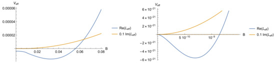
Figure 2. The effective potential for a vector field in a magnetic background. In the left panel, the mass is $m=0.1$, and in the right panel, it is $m=0$. The imaginary part is downscaled by a factor of 10. In the left panel, it sets in at $B=0.01$ and in the right panel at $B=0$.

3.4. Possible Instabilities in QED in a Magnetic Background Field

In the preceding subsection, we discussed some effects caused by the contribution from the ‘tr ln’ to the effective Lagrangian. There, it was sufficient to know the spectrum of the kernel of the free action, Equations (16), (27) and (44). In this subsection, we focus on QED in a magnetic background, including higher-order corrections in the form of anomaly factor (26).

A preliminary remark may be in order. At the end of the 1970s, there were claims that pair creation might be possible in pure magnetic fields. As well known, in a strong electric field, say a Coulomb field with $Z>137$, the gap between electron and positron ground state levels will close, and these levels cross. May a similar instability be possible in some inhomogeneous magnetic fields as well? Some years later, Ref. [13] showed that this is not possible in principle.

The discussion is quite simple and rests on the fact that the momentum operator

$$\begin{array}{c}\hfill \stackrel{\sim }{\mathbf{ß}}=(\overrightarrow{p}-e\overrightarrow{A})\end{array}$$

(98)

is Hermite. Squaring the Dirac equation,

$$\begin{array}{c}\hfill (\overrightarrow{\alpha }\stackrel{\sim }{\mathbf{ß}}+\beta m)\psi =E\psi \Rightarrow ({(\overrightarrow{\alpha }\stackrel{\sim }{\mathbf{ß}})}^2+m^2)\psi =E^2\psi ,\end{array}$$

(99)

(in three dimensional notations, $\alpha ={\gamma }^0\overrightarrow{\gamma }$, $\beta ={\gamma }^0$), a trivial rewriting into the form ${(\overrightarrow{\alpha }\stackrel{\sim }{\mathbf{ß}})}^2\psi =(E^2-m^2)\psi$ shows on the left side an operator with only non-negative eigenvalues. Hence, the energy cannot go below the mass. The above discussion is a special case of the Vafa–Witten theorem.

Now we turn to the first radiative correction for the effective Lagrangian. It is given by the ‘tr ln’ with the spectrum (27) without the anomaly factor and was considered in Section 3.3.2. This system is stable. However, including the anomaly factor, for strong fields, $H>H_c$, for example, in [14], pair creation was discussed. If taking $a_e$ as a constant, the gap $\Delta E=2m\left(1-a_e\frac{H}{H_c}\right)$, between electron and positron ground states, may close for sufficiently strong fields.

However, as pointed out in [15], the anomaly factor is a function of the background field and the state of the electron, (26) being its weak field approximation. In this approximation, the magnetic moment can be extracted from the triangle graph (as in [2]), which appears from expanding the electron self-energy graph. In a homogeneous magnetic field, this graph was calculated already in [16] for arbitrary field strength. In [15,17], its strong field approximation was calculated for the ground state energy, which was shown to grow quadratically with the logarithm of the magnetic field (for the excited states, it is linear in the logarithm). This way, the stability of QED was ensured.

The calculation of the electron energy, including the dependence on its state, was a topic of several papers, especially [18,19]. Special interest was in the synchrotron radiation in a magnetic field, which can be calculated in this context since for higher levels, the energy has an imaginary part.

The calculation of the anomaly factor requires knowledge of the electron self-energy (mass operator) in the magnetic background. There are basically two kinds of representations. The first rests on the expansion of the electron propagator in the eigenfunctions of the Dirac operator. It is also known as $E_p$-representation, where $E_p$ are the one-particle energies. This method is general and, in principle, applicable to any background. Now the homogeneous background with its high degree of symmetry allows for a more elegant approach, which was invented initially by [10]. It rests on the proper time representation of the inverse Dirac operator in the magnetic field in a similar way as it was applied to derive Equation (75). Viewing the exponential as an evolution operator, taken in corresponding matrix elements, one can derive ‘equations of motion’ and solve these. This representation, applied to the mass operator, had been used in [20]. After transforming to momentum space representation, they obtained in a very elegant way the formula

$$\begin{array}{cc}\hfill M& =\frac{\alpha }{2\pi }m{\int }_0^{\infty }\frac{dy}{y}{\int }_0^{1}du{e}^{-uy{H}_0/H}\left[-1-u+\frac{1+u{e}^{-2y}}{1-u+u{e}^{-y}sinh\left(y\right)/y}\right]\hfill \end{array}$$

(100)

for the mass operator in the ground state. $H_0=eH/m^2$ is the critical field strength. It is a double-parametric integral, as it is common for a loop with two lines. This integral is convergent; the necessary renormalization already occurred. The mass operator enters an effective Dirac equation and may be viewed as an addendum to (20). In the ground state, it adds to the energy,

$$\begin{array}{c}\hfill E_0=m+M,\end{array}$$

(101)

(the energies of the lowest Landau level and of the spin coupling cancel). Compared with a non-relativistic approximation of (27), one comes to its relation

$$\begin{array}{c}\hfill a_e=-\frac{1}{eH}M\end{array}$$

(102)

for the anomaly factor. In Figure 3, we show M, (101), as a function of the magnetic field. For a weak field, it lowers the energy, changing the sign before the critical field strength $H_c$ is reached.

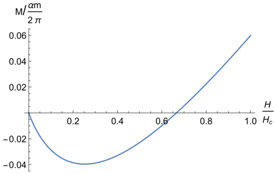
Figure 3. The mass correction M (100), divided by $\frac{\alpha m}{2\pi }$, i.e., the function I (A7), as a function of the magnetic field. In the minimum, this function takes small values and must be additionally multiplied by $\alpha$ to compare with the rest mass.

The calculation of the strong field limit of the mass operator has a quite long history. The first two terms of the asymptotic expansion, which are quadratic and linear in $lnH$, have been found independently by [15,17]. The constant contribution was calculated in [21]. We repeat this calculation in the Appendix B and show that it needs minor improvement.

4. Instabilities with First Radiative Correction

In a seminal paper [8], the question was raised on whether radiative corrections are able to cause an instability, or even more, a spontaneous symmetry breaking, in a massless theory. It was shown that radiative corrections do not leave massless theories such as scalar ${\varphi }^4$ or scalar electrodynamics without dimensional parameters. In the present section, we will discuss these ideas, which resulted, for instance, in the phenomenon of dimensional transmutation.

4.1. Instabilities in Scalar ${\varphi }^4$ Theory

We start with the Lagrangian of a scalar ${\varphi }^4$ model with a single real field $\varphi$,

$$\begin{array}{c}\hfill \mathcal{L}=\frac{1}{2}\varphi (-p^2-m^2)\varphi -\frac{\lambda }{4}{\varphi }^4.\end{array}$$

(103)

Distinct from (8), we have no background field here, and we use momentum representation. As before, the metric is Euclidean.

If $m^2>0$, the quantization is around $\varphi =0$, and after renormalization, m is the physical mass, which does not follow, such as the renormalized coupling $\lambda$, from the quantum theory, and one may calculate all quantum corrections in perturbation theory, at least in principle.

If $m^2<0$, if quantizing around $\varphi =0$, the ground state (vacuum) energy acquires an imaginary part already from the first radiative correction, and the system becomes unstable. For a constant field $\varphi$, the potential belonging to Lagrangian (103) has the ‘Mexican hat’ shape. The system will leave the ‘top of the hill’ and roll down to the bottom. Mathematically, this is realized by a shift,

$$\begin{array}{c}\hfill \varphi \to {\varphi }_c+\varphi ,\end{array}$$

(104)

of the field, and quantization around ${\varphi }_c$, which has the meaning of the vacuum expectation value of the field, ${\varphi }_c=⟨0\mid \varphi \mid 0⟩$, or the condensate. In general, the condensate may depend on coordinates. However, at least in the beginning, one considers a homogeneous condensate.

With the substitution (104), and $m^2\to -m^2$, Lagrangian (103) turns into

$$\begin{array}{c}\hfill \mathcal{L}=\frac{m^2}{2}{\varphi }_c^2-\frac{\lambda }{4}{\varphi }_c^4+{\varphi }_c(m^2-\lambda {\varphi }_c^2)\varphi +\frac{1}{2}\varphi (-p^2-M^2)\varphi -\lambda {\varphi }_c{\varphi }^3-\frac{\lambda }{4}{\varphi }^4\end{array}$$

(105)

with a new mass,

$$\begin{array}{c}\hfill M^2=-m^2+3\lambda {\varphi }_c^2.\end{array}$$

(106)

This Lagrangian has a linear contribution, which must vanish (we quantize after substitution (104) again around $\varphi =0$), i.e.,

$$\begin{array}{c}\hfill m^2=\lambda {\varphi }_c^2\end{array}$$

(107)

must hold on the tree level (this relation will be modified by the quantum corrections). At once, as can be seen easily, this is the condition for the minimum in ${\varphi }_c$ of the tree level part.

The first quantum correction is the ‘tr ln’-term in (54). Using (56), we obtain

$$\begin{array}{c}\hfill {\mathcal{L}}_{eff}=\frac{m^2}{2}{\varphi }_c^2-\frac{\lambda }{4}{\varphi }_c^4-V_{sc}\end{array}$$

(108)

with

$$\begin{array}{c}\hfill V_{sc}\left(M^2\right)=\frac{1}{2}\int \frac{d^{4}k}{{\left(2\pi \right)}^4}ln(k^2+M^2).\end{array}$$

(109)

This function is calculated in Appendix A. It has an ultraviolet divergence, and one must apply some regularization. In the Appendix A, we represent two of them, the zeta functional one and the momentum cut-off. The first one is more elegant while the second provides more physical insight. To demonstrate the ideas behind the renormalization, in this subsection, we use the second one.

Inserting $M^2$, (106), into (A4),

$$\begin{array}{cc}\hfill V_{sc}& =\frac{1}{64{\pi }^2}[-9{\lambda }^2{\varphi }_c^4\left(ln{\Lambda }^2+\frac{1}{2}\right)+\lambda {\varphi }_c^2\left(6m^2\left(ln{\Lambda }^2-\frac{1}{2}\right)\right)\hfill \\ \hfill & +{\Lambda }^4\left(ln{\Lambda }^2-\frac{1}{2}\right)-2m^2{\Lambda }^2-m^4\left(ln{\Lambda }^2+\frac{1}{2}\right)\hfill \\ \hfill & +M^{4}ln{M}^2],\hfill \end{array}$$

(110)

we reordered $V_{sc}$ by powers of the condensate ${\varphi }_c$ and a contribution, which is not a power of ${\varphi }_c$ since it contains the logarithm of $M^2$. The renormalization starts by considering the powers of ${\varphi }_c$ as counterterms and by absorbing them into the tree-level Lagrangian by the substitutions

$$\begin{array}{cc}\hfill \lambda & \to \lambda +\frac{9\lambda }{16{\pi }^2}\left(ln{\Lambda }^2+\frac{1}{2}\right),\hfill \\ \hfill m^2& \to m^2+12\lambda \left(m^2\left(ln{\Lambda }^2-\frac{1}{2}\right)+{\Lambda }^2\right).\hfill \end{array}$$

(111)

The second line in (110) does not depend on ${\varphi }_c$ and can be added as a constant term to the Lagrangian. We do not show this explicitly. Moreover, the specific form of substitution such as (111) is unimportant, and we will not show them in the following. It is only important that such substitutions are possible. We mention that the substitutions (111) become infinite ones in the limit of removing the regularization, $\mathrm{\Lambda }\to \infty$. When performing the corresponding substitutions with the zeta functional regularization, i.e., with $V_{sc}$ as given by (A2), these will be finite.

As known, regularization introduces a new, arbitrary dimensional factor. In the cut-off regularization, it is $\mathrm{\Lambda }$ that has the dimension of momentum, and in the zeta functional regularization, it is $\mu$, as mentioned in Section 3.2. This circumstance opens the possibility of finite renormalization. Usually, such arbitrariness is fixed by so-called normalization conditions, which need a physical interpretation or justification. We mention that changes in these conditions, or in the regularization parameters, can be described in terms of the renormalization group. For instance, the factor in front of the logarithm in the upper line in (111) is the first coefficient in the so-called $\beta$ function. The renormalization group plays an important role in quantum field theory, but it is also outside the scope of this review.

Using the renormalization freedom, we take the ‘tr ln’ contribution in the form

$$\begin{array}{c}\hfill V_{sc}\left(M^2\right)=\frac{1}{64{\pi }^2}\left[4m^2+2M^2\left(ln\frac{M^2}{2m^2}-\frac{3}{2}\right)\right].\end{array}$$

(112)

It is motivated by the tree level minimum, which remains unchanged when including this $V_{sc}$ since it was chosen such that the normalization conditions

$$\begin{array}{c}\hfill V_{sc}{\left(M^2\right)}_{|m^2=\lambda {\varphi }_c^2}=0,{\frac{\partial V_{sc}\left(M^2\right)}{\partial M^2}}_{|m^2=\lambda {\varphi }_c^2}=0,\end{array}$$

(113)

hold.

Now we can discuss the interpretation of these results. With (57), we obtain an effective potential, including the first radiative correction, in the form

$$\begin{array}{c}\hfill V_{eff}=-\frac{m^2}{2}{\varphi }_c^2+\frac{\lambda }{4}{\varphi }_c^4+V_{sc}\left(M^2\right)\end{array}$$

(114)

with $M^2=-m^2+3\lambda {\varphi }_c^2$. Considered as a function of ${\varphi }_c$, it has a minimum at ${\varphi }_c=m/\sqrt{\lambda }$, and the mass M takes in this minimum the value $M=\sqrt{2}m$. It is real. This way, one has a consistent theory with a condensate. For our needs, this is sufficient. We mention that this approach allows for the inclusion of temperature (via the Matsubara representation) and the study of symmetry restoration with a rising temperature. In doing so, infrared problems occur that require the inclusion of an infinite number of higher radiative corrections (graphs). All this is outside the given review. The interested reader may consult [22] for a general introduction and motivation, Ref. [23] for the summation formalism, and the most recent paper [24] for the actual state and for further literature.

Finally, we discuss the massless case, $m=0$, which was the original motivation for [8]. In that case, model (103) does not have any dimensional parameter. As already mentioned, such a parameter comes in with regularization. All previous discussions and formulas are applicable until (112), where formally putting $m\to 0$ would produce an infinity. There is no reasonable normalization condition opposite to the massive case. In connection with the Casimir effect, this point was discussed in detail in [7] (Section 4.3). Here, we take $V_{sc}$ in the form

$$\begin{array}{c}\hfill V_{sc}=\frac{9{\lambda }^2{\varphi }_c^4}{64{\pi }^2}\left(ln\frac{{\varphi }_c^2}{{\mu }^2}-\frac{25}{6}\right),\end{array}$$

(115)

where $\mu$ is arbitrary. The complete one-loop effective potential reads

$$\begin{array}{c}\hfill V_{eff}=\frac{\lambda }{4}{\varphi }_c^4+\frac{9{\lambda }^2{\varphi }_c^4}{64{\pi }^2}\left(ln\frac{{\varphi }_c^2}{{\mu }^2}-\frac{25}{6}\right).\end{array}$$

(116)

Following [8], we took $\frac{1}{6}{\frac{d^4{V}_{eff}}{d{\varphi }_c^4}}_{|{\varphi }_c=\mu }=\lambda$ as the normalization condition (note, their coupling $\lambda$ is our $\lambda /6$).

This function has the interesting property that from the logarithm for small ${\varphi }_c$ negative contributions appear, which result for

$$\begin{array}{c}\hfill {{{\varphi }_c}^2}_{|min}=\frac{{\mu }^2}{3\lambda }exp\left(\frac{11}{6}-\frac{8{\pi }^2}{9\lambda }\right)\end{array}$$

(117)

in a minimum,

$$\begin{array}{c}\hfill {V_{eff}}_{|min}=-\frac{9{\lambda }^2{\mu }^4}{128{\pi }^2}exp\left(\frac{22}{3}-\frac{32{\pi }^2}{9\lambda }\right).\end{array}$$

(118)

Formally, this is to the right from the tree level minimum at ${\varphi }_c=0$. However, in the perturbative approach, this is exponentially small and must be considered as zero. For the minimum to exit, the logarithm must be negative and of the same order as the tree contribution in (116), i.e., perturbatively small. This can be achieved only by a very small condensate ${\varphi }_c$.

In [8], one finds another, even more convincing explanation. By improving (117) by the renormalization group equation, or by letting the coupling constant run, negative values of the effective potential occur only for ${\varphi }_c$ in a region beyond the Landau pole, hence in a nonphysical region.

In summary, in this section, we have seen that in a pure scalar theory, an instability may occur when the initial mass has a negative, nonzero square. This instability results in a condensate. This phenomenon can be viewed as the scalar part of the Higgs phenomenon. In case the initial mass is zero, no realistic minimum and no condensate appear.

4.2. Scalar QED and Abelian Higgs Model

In this section, we consider the massless scalar QED. Its Lagrangian reads

$$\begin{array}{c}\hfill \mathcal{L}=-\frac{1}{4}{F}_{\mu \nu }^2+{\left(D_{\mu }\varphi \right)}^{*}\left(D_{\mu }\varphi \right)-\frac{\lambda }{2}{\left({\varphi }^{*}\varphi \right)}^2,\end{array}$$

(119)

where $F_{\mu \nu }={\partial }_{\mu }{A}_{\nu }-{\partial }_{\nu }{A}_{\mu }$ is the field strength of the electromagnetic field, and $\varphi$ is a complex scalar field. With the covariant derivative

$$\begin{array}{c}\hfill D_{\mu }={\partial }_{\mu }-ie{A}_{\mu },\end{array}$$

(120)

this Lagrangian is invariant under the group U(1). Regarding (8), the electromagnetic field is now a dynamic one, and we added the self-interaction of the scalar field. This model is a generalization of the pure scalar model considered in the preceding subsection. It is also called the Abelian Higgs model for the spontaneous symmetry breaking that it allows.

Following the ideas of [8], we turn to real fields ${\varphi }_i$,

$$\begin{array}{c}\hfill \varphi =\frac{1}{2}({\varphi }_1+i{\varphi }_2),\end{array}$$

(121)

and rewrite the Lagrangian in the form

$$\begin{array}{c}\hfill \mathcal{L}=\frac{1}{2}{A}_{\mu }\left({\partial }^2{\delta }_{\mu \nu }-{\partial }_{\mu }{\partial }_{\nu }\right)A_{\nu }+\frac{1}{2}{({\partial }_{\mu }{\varphi }_1+e{A}_{\mu }{\varphi }_2)}^2+\frac{1}{2}{({\partial }_{\mu }{\varphi }_2-e{A}_{\mu }{\varphi }_1)}^2-\frac{\lambda }{8}{({\varphi }_1^2+{\varphi }_2^2)}^2.\end{array}$$

(122)

It has, in addition to the gauge symmetry, O(2) symmetry, and its scalar part is a special case of an O(2N) model.

Like in the scalar case, we imagine a mass term added with a negative mass square. This would result in an instability and force us to consider the possibility of having a condensate. Therefore, we make a shift

$$\begin{array}{c}\hfill {\varphi }_i\to \frac{1}{\sqrt{2}}{\varphi }_c+{\varphi }_i,\end{array}$$

(123)

of the scalar fields. Thereby, we follow [8], slightly changing the notations. In general, any shift away from the origin in the (${\varphi }_1,{\varphi }_2$)-plane would be as good as 4.2.5.

With (123), the Lagrangian turns into

$$\begin{array}{cc}\hfill \mathcal{L}& =-\frac{\lambda }{4}{\varphi }_c^2+\frac{1}{2}{A}_{\mu }\left(({\partial }^2-e^2{\varphi }_c^2){\delta }_{\mu \nu }-{\partial }_{\mu }{\partial }_{\nu }\right)A_{\nu }+\frac{1}{2}{\varphi }_1\left({\partial }^2-2\lambda {\varphi }_c^2\right){\varphi }_1+\frac{1}{2}{\varphi }_2\left({\partial }^2-2\lambda {\varphi }_c^2\right){\varphi }_2\hfill \\ & -\frac{1}{\sqrt{2}}{\varphi }_{c}e{A}_{\mu }{\partial }_{\mu }({\varphi }_1-{\varphi }_2)-\lambda {\varphi }_c^2{\varphi }_1{\varphi }_2+\dots ,\hfill \end{array}$$

(124)

where the dots stand for interaction terms that we do not need to consider (after performing the shift). In addition, we did not show the terms that are linear in the fields since these must vanish in the extremum of the Lagrangian. Equation (124) shows the constant and the quadratic parts of the Lagrangian. However, it has two cross-terms. The first one disappears when using the symmetry ${\varphi }_1\leftrightarrow {\varphi }_2$ between the scalar fields. The second can be diagonalized by the substitution ${\varphi }_1\to \frac{1}{\sqrt{2}}({\varphi }_1+{\varphi }_2)$, ${\varphi }_2\to \frac{1}{\sqrt{2}}(-{\varphi }_1+{\varphi }_2)$, which results in

$$\begin{array}{cc}\hfill \mathcal{L}& =-\frac{\lambda }{4}{\varphi }_c^2+\frac{1}{2}{A}_{\mu }\left(({\partial }^2-e^2{\varphi }_c^2){\delta }_{\mu \nu }-{\partial }_{\mu }{\partial }_{\nu }\right)A_{\nu }+\frac{1}{2}{\varphi }_1\left({\partial }^2-\lambda {\varphi }_c^2\right){\varphi }_1+\frac{1}{2}{\varphi }_2\left({\partial }^2-3\lambda {\varphi }_c^2\right){\varphi }_2.\hfill \end{array}$$

(125)

After the shift, the electromagnetic field acquires a mass $e^2{\varphi }_c^2$, and the scalar fields acquires masses $\lambda {\varphi }_c^2$ and $3\lambda {\varphi }_c^2$.

Now we calculate the effective potential. For the ‘tr ln’ contributions, we use Formula (115) for all modes,

$$\begin{array}{c}\hfill V_{eff}=\frac{\lambda }{4}{\varphi }_c^2+\left(\frac{5{\lambda }^2}{32{\pi }^2}+\frac{3e^4}{64{\pi }^2}\right){\varphi }_c^4\left(ln\frac{{\varphi }_c^2}{{\mu }^2}-\frac{25}{6}\right),\end{array}$$

(126)

and take into account that the electromagnetic field now has three polarizations.

We look for a minimum of this effective potential and discuss, such as in the preceding subsection, the tree level and the quantum correction, which should be of the same order. Demanding that the logarithm is of order one, this requires

$$\begin{array}{c}\hfill \lambda \sim e^4.\end{array}$$

(127)

With such a relation, we have ${\lambda }^2\sim e^8<<e^4$, and (36) simplifies,

$$\begin{array}{c}\hfill V_{eff}=\frac{\lambda }{4}{\varphi }_c^2+\frac{3e^4{\varphi }_c^4}{64{\pi }^2}\left(ln\frac{{\varphi }_c^2}{{\mu }^2}-\frac{25}{6}\right).\end{array}$$

(128)

For the arbitrary constant $\mu$, we take the value of the effective potential, $\mu ={\varphi }_{c,min}$, and from the first derivative of (127), we arrive at

$$\begin{array}{c}\hfill \lambda =\frac{11e^4}{16{\pi }^2}\end{array}$$

(129)

which confirmed (127). The potential in this minimum is

$$\begin{array}{c}\hfill {V_{eff}}_{|min}=-\frac{3e^4}{128{\pi }^2}{\left({\varphi }_{c,min}\right)}^4.\end{array}$$

(130)

The interpretation of ${\varphi }_{c,min}$ is that it is the vacuum expectation of the field, ${\varphi }_{c,min}=⟨0\mid \varphi \mid 0⟩$ ${\varphi }_{c,min}={⟨\varphi ⟩}_0$, so that with (129), the effective potential finally takes the form

$$\begin{array}{c}\hfill V_{eff}=\frac{3e^4{\varphi }_c^4}{64{\pi }^2}\left(ln\frac{{\varphi }_c^2}{{⟨\varphi ⟩}_0^2}-\frac{1}{2}\right).\end{array}$$

(131)

We started this subsection with Lagrangian (119). It has two parameters, the pair ($\lambda ,e$) of dimensionless couplings. We ended with the effective potential (41), which has the parameter pair (${\varphi }_c,e$). Now ${\varphi }_c$ has a dimension. It has an arbitrary parameter coming in with regularization and for which we take ${\varphi }_{c,min}$. In [8], the change from the dimensionless $\lambda$ to the dimensional ${\varphi }_c$ is called dimensional transmutation. In addition, they showed that in this case, application of the renormalization group does not remove the minimum.

The outcome from this subsection is the understanding that by adding an Abelian vector field to the scalar sector, a condensate and symmetry breaking occur, as shown in Figure 4. Thereby, the initial coupling $\lambda$, which should obey relation (127), drops out from the final result (131), and, unlike the pure scalar model, renormalization group improvement does not destroy this picture.

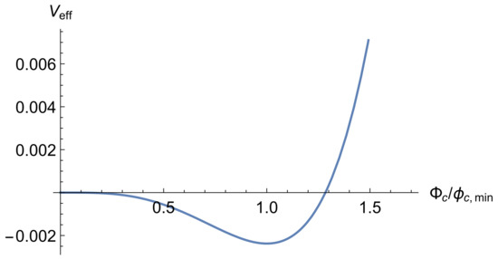
Figure 4. The effective potential (131) of the Abelian Higgs model (119).

It is interesting to look at the fate of the modes under the symmetry breaking. Initially, we have two photon modes and two scalar modes. After the symmetry breaking, one scalar mode goes into massive photon mode, and the other remains. This can be seen, for instance, using a module-phase representation, $\varphi =\rho e^{i\mathrm{\Theta }}$. The field $\mathrm{\Theta }$ is massless and represents the Goldstone boson. However, together with the electromagnetic sector, it appears as a pure gauge and can be eliminated. A similar discussion can be found in [25] as well as in the discussion of further developments.

Of course, there are further developments of this model. The most important is the inclusion of finite temperature. One needs to perform resummation to eliminate infrared problems. In the result, as shown in [26], a first-order phase transition shows up, and the symmetry is restored when raising the temperature. A physically important extension is the electroweak phase transition (or crossover as the lattice calculations suggest), which is still a topic under actual discussion [27].

4.3. Instabilities in Non-Abelian Gauge Theories

In this subsection, we consider instabilities in non-Abelian gauge theories. The most relevant are QCD and the electroweak theory. Both involve non-Abelian vector fields, which have in a magnetic background a spectrum such as in (44) or (83). Its peculiarity results from their spin, $s=1$, which causes a coupling to a magnetic background field with negative energy. Frequently, this property is discussed as anti-screening or paramagnetism. In QCD, which is a massless theory, the result is a tachyonic state that is present for any strength of the background field making the ground state, which is considered a Savvidy vacuum, unstable. This case was discussed in Section 3.3.3. The depths of the minimum (97), of the effective potential are as shallow as in the massless scalar case in Section 4.1, Equation (118), namely exponentially decreasing for small coupling. However, unlike the scalar case, it is not washed out by renormalization group improvement due to asymptotic freedom.

In the electroweak theory, the mass $m_W$ of the W-boson postpones the instability until the field strength reaches the critical value $H_c=m_W/g$, i.e., until the background field becomes very strong.

In the literature, the instability was discussed mainly in the context of an applied magnetic field, which would cause pair production and could have cosmological implications. The spontaneous generation of a magnetic field is not considered due to the large mass threshold. The topic was intensively discussed at the beginning of the 1980s, i.e., long before the discovery of the Higgs boson, for instance in [28,29,30,31]. Therefore, all parameter regions were of interest. A much-discussed question, for instance in [29], was the gauge fixing to be applied in the background field, unitary gauge or the $R_{\xi }$-gauge. Both are possible and deliver, finally, the same result.

As an example of these developments, we consider [30]. The model consists of an SU(2)-field coupled to a triplet of Higgs fields. Combining (31) and (119), the Lagrangian reads

$$\begin{array}{c}\hfill \mathcal{L}=-\frac{1}{4}{\left(F_{\mu \nu }^a\right)}^2+\frac{1}{2}\mid D_{\mu }^{ab}{\varphi }^a{\mid }^2-\frac{m^2}{2}{\varphi }^a{\varphi }^a-\frac{\lambda }{4}{\left({\varphi }^a{\varphi }^a\right)}^2,\end{array}$$

(132)

where the covariant derivative,

$$\begin{array}{c}\hfill D_{\mu }^{ab}=\partial {\delta }^{ab}+g{ϵ}^{}acb(A_{\mu }^c+B_{\mu }^c)\end{array}$$

(133)

provides the coupling to both, the background field $B_{\mu }^a$ and gauge potential $A_{\mu }^a$. Following (41), we rotate the fields,

$$\begin{array}{c}\hfill W_{\mu }=\frac{1}{\sqrt{2}}(A_{\mu }^1+i{A}_{\mu }^2),\varphi =\frac{1}{\sqrt{2}}({\varphi }^1+i{\varphi }^2),\end{array}$$

(134)

and keep the third component. Thereby, the derivative term of the Higgs field turns into

$$\begin{array}{c}\hfill \frac{1}{2}\mid D_{\mu }^{ab}{\varphi }^a{\mid }^2=\mid ({\partial }_{\mu }-ig(A_{\mu }^3+B_{\mu }^3))\varphi {\mid }^2+\frac{1}{2}\mid ({\partial }_{\mu }-ig{W}_{\mu }){\varphi }^3{\mid }^2,\end{array}$$

(135)

the mass and self-interaction terms, accordingly, into

$$\begin{array}{cc}\hfill -\frac{m^2}{2}{\varphi }^a{\varphi }^a& =-m^2{\varphi }^{*}\varphi -\frac{m}{2}{\left({\varphi }^3\right)}^2,\hfill \\ \hfill -\frac{\lambda }{4}{\left({\varphi }^a{\varphi }^a\right)}^2& =-\lambda {\left[{\varphi }^{*}\varphi ++\frac{1}{2}{\left({\varphi }^3\right)}^2\right]}^2.\hfill \end{array}$$

(136)

The spontaneous symmetry breaks sets after changing the sign of the mass square, $m^2\to -m^2$, such as in Section 4.1, with a shift of the third component of the Higgs field,

$$\begin{array}{c}\hfill {\varphi }^3\to {\varphi }_c+{\varphi }^3.\end{array}$$

(137)

From (135), the W-field acquires a mass, $m_W=g^2{\varphi }_c^2$, in addition to what we have seen in Section 4.2.

Now we have a charged vector field with mass $m_W$ and a charged scalar with mass $3\lambda {\varphi }_c^2$ in the magnetic background, with $A_{\mu }^3$ as a neutral vector field and ${\varphi }^3$ as a neutral scalar field. The first two contribute with their spectrum in analogy to (83) and (64), as well as two modes from $A_{\mu }^3$ and one mode from ${\varphi }^3$, such as (109), to the one-loop effective potential. On the given level, all contributions are additive.

We demonstrate as an example the result obtained in [30] in this situation. The following expression for the effective Lagrangian was obtained

$$\begin{array}{c}\hfill {\mathcal{L}}_{eff}=-\frac{B^2}{2}-\frac{7g^2{B}^2}{32{\pi }^2}\left(ln\frac{gB}{4\pi {\mu }^2}+c\right)-\frac{m_W^2}{16{\pi }^2}V\end{array}$$

(138)

with $c=\gamma -1-\frac{1}{7}(12{\zeta }^{\prime }(-1)+2ln2+\frac{2}{3})$ and where

$$\begin{array}{cc}\hfill V& =\frac{3}{2}{\varphi }^4\left(ln{\varphi }^2-\frac{1}{2}\right)+\frac{g^2{B}^2}{2m_W^2}[-3(m^{4}ln{m}^2+\frac{1}{2}+ln2)+24{\zeta }^{\prime }(-1,\frac{m^2+1}{2})\hfill \\ \hfill & +12{\zeta }^{\prime }(-1)+ln2+4(m^2+1)ln(m^2+1)-4(m^2-1)ln(m^2-1)].\hfill \end{array}$$

(139)

In their notations, $m^2=\frac{2m_W^2{\varphi }^2}{B^2}$, and $\varphi$ is the scalar condensate. For the numerical evaluation, it is meaningful to use the relation

$$\begin{array}{c}\hfill {\zeta }^{\prime }(-1,z)={\zeta }^{\prime }(-1)-ln{\Gamma }_B\left(z\right)+zln\Gamma \left(z\right).\end{array}$$

(140)

The corresponding effective potential, normalized to $B=0$, is shown in Figure 5 as a function of the condensate $\varphi$ for two values of the magnetic field. The solid line represents the real part, and the dashed line is the imaginary part. It is clearly seen that for small B, the effective potential is real and shows the minimum known from the Abelian Higgs model. For a larger magnetic field, an additional minimum appears near the origin together with an imaginary part. This minimum corresponds to that known from the Savvidy vacuum, and it becomes the deeper one. In addition, it is seen that the magnetic minimum is much shallower than the scalar one. For the picture, quite a large value of the coupling was chosen to obtain both minima shown in one picture.

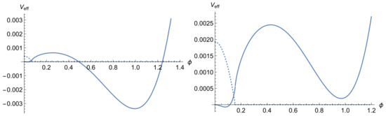
Figure 5. The effective potential $-{\mathcal{L}}_{eff}$ (138) as a function of the scalar condensate $\varphi$, for $m_W=1$, $g=1$ and $\mu =1$. In the left panel, the magnetic field is $B=0.1$, and in the right panel $B=0.22$. The dashed line is the imaginary part.

Similar pictures were obtained in [32], where, however, the focus was on the formation of a lattice of magnetic flux lines. At the beginning of the 1980s, there were a number of investigations of the effective potential. For instance, in [31], similar pictures were obtained, but there was a question about the symmetry restoration by a large magnetic field, partly by early discussions in [33]. Similar discussions can be found in [28,34]. In [35], it was argued that this is not possible as long as the ground state is not stable. The magnetic vacuum remains, as seen, for example, in the right panel in Figure 5, as well as the scalar condensate with it, in this minimum for all values of the magnetic field. Before the discovery of the Higgs boson, investigation of the effective potential of the electroweak model in a magnetic field was used to obtain bounds on the Higgs mass; for a review see [36].

The question of symmetry restoration was also investigated at finite temperatures. The general expectation, according to Refs. [37,38], was that broken symmetry, the spontaneous creation of a magnetic field in our case, will be restored at a sufficiently high temperature. However, as found in [39,40], this is not the case.

4.4. Electroweak Magnetism

Beyond the instabilities caused by the one-loop corrections, it is also interesting to study non-Abelian fields on the classical level. As an especially intriguing feature, in quite a number of papers, the analogy to a (dual) superconductor was considered. In this spirit, the question arises of how the field responds to an applied homogeneous magnetic field. Will this response be a lattice of flux lines or something else? The first discussion of this question can be found in [41]. It was assumed that domains will form in the plane perpendicular to the applied field with a size smaller than that necessary for the formation of an unstable mode. Thereby, formation of the unstable mode is considered an infrared, long-range effect. These domains are formed by magnetic flux tubes. In order to restore Lorentz invariance of the model, in [41], a model was developed with a fluid-like superposition of the flux tubes. However, this model, which is known as the “Copenhagen vacuum”, was criticized independently in [40,42] and was finally abandoned.

The formation of the lattice of flux lines is of interest in the electroweak theory. In [43], a mechanism was discussed that goes beyond the quadratic approximation and involves the interaction with a longitudinal mode of the W-field. In [44], the condensate was discussed in the Georgi–Glashow model. In a linearized approximation, the existence of a vortex-like condensate was confirmed, and the relation to a type II superconductor was discussed. In [45], these results were discussed in the electroweak model near the Bogomolny bound

$$\begin{array}{c}\hfill \lambda =\frac{g^2}{8{cos}^2{\mathrm{\Theta }}_W}\end{array}$$

(141)

where $\lambda$ is the Higgs coupling constant, and ${\mathrm{\Theta }}_W$ is the Weinberg angle. In [35], similar results were reported using a perturbative expansion near the bound. As a result, it was concluded that beyond the critical field strength, a periodic lattice of flux lines will be formed.

To demonstrate these ideas, we give a representation of the basic methods used. First, we consider the derivation of exact (classical) equations of motion for the tachyonic modes, which are a breakdown of the general Yang–Mills equations for this specific component. Second, we represent the attempts to lower the effective potential by some superposition of tachyonic modes.

4.4.1. Equations of Motion for the Tachyonic Mode

In [44], a restricted model was discussed. It has an O(3) symmetry, and it is similar to the SU(2)-model considered in Section 2.4 with an additional mass term for the W-field,

$$\begin{array}{cc}\hfill \mathcal{L}& =-\frac{1}{4}{\left(F_{\mu \nu }^a\right)}^2-m^2{W}_{\mu }^{*}{W}_{\mu }.\hfill \end{array}$$

(142)

The fields are a charged vector field $W_{\mu }$ and a neutral vector field $A_{\mu }$, related to the initial fields $A_{\mu }^a$ by the relation (41). The W-field stands for the W-boson and the A-field for the electromagnetic field. Restricting the mode carries the instability

$$\begin{array}{c}\hfill W_1=W,W_2=iW,f_{12}=-f_{21},\end{array}$$

(143)

which are the only non-vanishing components. In this case, and assuming dependence on $x_{1,2}$ only, the field equations can be simplified. This calculation is shown in Appendix C. Finally, the equations for mode (143) read

$$\begin{array}{cc}\hfill -({\partial }_1^2+{\partial }_2^2)ln\left|W\right|& =m^2+2e^2{\left|W\right|}^2,\hfill \\ \hfill f_{12}& =\frac{m^2}{e}+2e{\left|W\right|}^2.\hfill \end{array}$$

(144)

The first line is a Liouville-type equation for the W-field, and the second line gives the expression for the magnetic field in terms of the W-field. The energy of the solutions can be expressed in the form

$$\begin{array}{c}\hfill E_{cl}=\frac{H_{cr}^2}{2}+2e{H}_{cr}{\left|W\right|}^2,\end{array}$$

(145)

where $H_{cr}=m^2/2$ is the critical field strength. This way, the classical energy is always non-negative, as one should expect. We also mention that the system can be rewritten in terms of first-order equations using (A25) and the field strength $F_{12}$ in addition to the second line in (144). The system of equations, generalizing the above ones to the case of the bosonic part of the electroweak theory, was derived in [45]. A review and further discussions in [46] focused especially on the interpretation of the second line in (144). The plus sign on the second term, which is an enhancement of the applied magnetic field by the system, is interpreted as anti-screening caused by the asymptotic freedom.

4.4.2. A Lattice of Flux Lines

In this subsection, we consider the formation of a lattice of magnetic flux lines such as that in a type II superconductor. We follow the first attempt of this kind [47]. The authors start with a background field in the Landau gauge such as in (11). The equation for the tachyonic mode follows as a special case from ${\mathcal{L}}_2$ (42). The general solution is a superposition of harmonic oscillator ground state functions,

$$\begin{array}{c}\hfill W\left(x\right)=\int \frac{d{k}_2}{2\pi }\frac{d{k}_3}{2\pi }\tilde{\varphi }(k_2,k_3)e^{-i(k_2{x}_2+k_3{x}_3)}exp\left[-\frac{eH}{2}{\left(x_1-\frac{k_2}{eH}\right)}^2\right],\end{array}$$

(146)

where $\tilde{\varphi }(k_2,k_3)$ is an arbitrary coefficient function. All these states have the same energy and realize the degeneracy of the ground state.

In [47], two ‘naive’ choices for $\tilde{\varphi }$ are discussed,

$$\begin{array}{c}\hfill \tilde{\varphi }(k_2,k_3)\sim \delta \left(k_2\right)\delta \left(k_3\right),\mathrm{or}\tilde{\varphi }(k_0,k_2,k_3)\sim \delta \left(k_3\right).\end{array}$$

(147)

In the first case, the solution describes a magnetic field with a Gaussian shape on the plane $x_1$ = 0. In the second case, performing the Gaussian integration over $k_2$, a similar picture appears on the $x_2$ plane. In either case, the field is of finite size in one direction. The classical energy has translational invariance in all three spatial directions and is proportional to the corresponding lengths, ∼$L_1{L}_2{L}_3$, whereas the energy of the naive solutions is proportional only to two, say ∼$L_2{L}_3$. Thus, one needs to look for a superposition that would be proportional to the classical energy. With this motivation, the following ansatz was made,

$$\begin{array}{c}\hfill \tilde{\varphi }(k_2,k_3)=\Phi \delta \left(k_3\right)\sum _{m\in Z}\delta (k_2-mc),\end{array}$$

(148)

where $\Phi$ and c are some constants. For $c\gtrsim \frac{1}{\sqrt{eH}}$, we obtain an infinite set of leaves each with a Gaussian magnetic field. For $c\sim \frac{1}{\sqrt{eH}}$, an interference sets in, which will be constructive for $exp(-imc{x}_2)=1$. Inserting (148) into (146) results in

$$\begin{array}{c}\hfill W\left(x\right)=\Phi \sum _{m\in Z}exp\left[-\frac{c^2}{2eH}{m}^2-icm(x_2+i{x}_1)-\frac{eH}{2}{x}_1^2\right].\end{array}$$

(149)

With the notations, $v=-\frac{c}{2\pi }(x_1+i{x}_2)$, $q=exp(-\frac{c^2}{2eH})$, one comes to a representation in terms of a Theta function,

$$\begin{array}{c}\hfill W\left(x\right)=\Phi {\theta }_3(v,q)exp\left[-\frac{eH}{2}{x}_1^2\right].\end{array}$$

(150)

This solution forms a regular lattice of magnetic flux lines. Further, in an ingenious calculation, Ref. [47] calculated the classical energy of this configuration, using an expression for the energy density derived earlier in [48], and came to the result

$$\begin{array}{c}\hfill E_{cl}=\frac{H^2}{2}-\frac{eH}{2\kappa }{|\Phi |}^2+\frac{e^2}{4\sqrt{\kappa }}{\theta }_3{(0,q)}^2{|\Phi |}^2\end{array}$$

(151)

with $\kappa =\frac{c^2}{2\pi eH}$. In hindsight, this formula should be a special case of 4.4.21.

Finally, the quantum contribution was added. For this, the one-loop vacuum energy in a homogeneous background was taken. The corresponding expression is, with the reversed sign, the second term in (96). This is, of course, a crude approximation. For the magnetic field, some average of (150) can be taken, which will not have an essential influence on the final result.

For the thus-obtained total energy, a minimum was found by a variation of all parameters entering, for instance, the coupling parameter e. As a result, an effective potential in the minimum was found ($q_0=e^{-\pi }$),

$$\begin{array}{c}\hfill {V_{eff}}_{|min}=\frac{11}{96{\pi }^2}{\Lambda }^4\left(-1+\frac{1}{{\theta }_3(0,q_0)}\right)exp\left(\frac{1}{{\theta }_3(0,q_0)-1}\right).\end{array}$$

(152)

With ${\theta }_3(0,q_0)\simeq 1.2713$, this effective potential is negative. The depth of this minimum is not decreasing, unlike in (97), and for small coupling, it will certainly become the deeper one.

The above ideas were also applied to the electroweak theory, for instance in [32]. Here, a decisive parameter is the ratio $K=\frac{m_H^2}{m_W^2}$, where $m_H$ is the Higgs mass and $m_W$ is the W-boson mass. For $K<1$ (these masses were not known at that time), an instability and a first-order phase transition similar to the Abelian Higgs model was found. In the opposite case, the magnetic instability sets in when the magnetic background field exceeds the critical value $H_c=m_W^2/e$ set by the W-boson mass. Making a perturbative expansion for small $e(H-H_c)$, the formation of a lattice of magnetic flux lines was derived, which is similar to the Abrikosov lattice in a superconductor. The formation of such a lattice was confirmed in [45] for the case of $m_H=m_Z$, where $m_Z$ is the Z-boson mass, using the Bogomolny method, i.e., by reducing the equations of motion to first-order equations that are easier to solve.

The above results have been reconsidered several times, the latest in [49]. The ansatz (146) had been modified using the symmetric gauge so that the initial solution describes a flux line (in place of a flux plane). The superposition of such solutions is then directly in terms of the center position. In addition, a regular lattice of these flux lines was chosen. It is argued that the time evolution of an initially homogeneous field would result in such a lattice. Then, the energy of such a configuration was minimized with respect to the scale parameter $\Phi$ of the solutions. Numerically, a minimum was found that is appreciably below the energy of the homogeneous field (the authors call it ‘classical field’).

In summary, there is a variety of instabilities in theories involving non-Abelian fields. In electroweak theory, due to the W-boson mass, the threshold for these is far beyond reachable energies (at least on Earth). In all cases, a spontaneous generation of a magnetic field is energetically favorable. However, these states are all unstable. A solution for the problem caused by this instability has not yet been found, despite numerous attempts, the latest being [50] in the massless case.

4.5. On the Fate of a Homogeneous Background Field

Being interested in non-perturbative, infrared effects, homogeneous fields are a prime candidate for a background field. Not only do such fields allow for quite explicit calculations, inhomogeneities tend to increase the classical energy. The general properties of background fields in an SU(2) theory were discussed in detail in [51]. It was shown that there are two types of translational invariant fields, of non-Abelian type, where the potential $A_{\mu }^a$ is constant in a suitable gauge, and an Abelian type field that may be taken in the form $A_{\mu }^a=-\frac{1}{2}{F}_{\mu \nu }{x}^{\nu }{\delta }^{a3}$, where $F_{\mu \nu }$ is a constant field strength. For the first type, it was shown that any constant potential with a non-vanishing field strength yields an unstable action, and for that from the second type, only Euclidean self-dual fields may be stable. These have infinitely many zero-mode excitations whose influence on the stability was left open. In addition, one should remember that self-duality in the Euclidean region implies an imaginary electric field in the Minkowski region.

The topic of a homogeneous Abelian background field was reconsidered independently a few years later in [52] from a variational point of view. The variations were taken in a class of fields being the unstable perturbations of a constant Abelian background, thereby including their quartic self-interaction. It was assumed that the stable fluctuations may be handled subsequently as perturbations. However, carrying out this program, it was observed that inclusion of the quartic terms resulted in a scaling of the coupling, which is different from the usual one that follows from the ultraviolet properties. In addition, it was mentioned that the inevitable mixing of the stable and the unstable modes could produce contributions of the same order as that from the unstable modes. Soon after, in [53], it was shown that the mixing of unstable and stable modes makes this procedure unreliable. More precisely, it was shown ‘that the minimum of the restricted action, $S(H_{\mu }+{\eta }_{\mu }^{\left(u\right)})$, is of no help’ ($H_{\mu }$ is the homogeneous background field and ${\eta }_{\mu }^{\left(u\right)}$ are the unstable fluctuations modes). Their discussion rests on the observation that there is no solution of the Yang–Mills equations of the form $H_{\mu }+{\eta }_{\mu }^{\left(u\right)}$ for non-vanishing ${\eta }_{\mu }^{\left(u\right)}$. This way, all attempts to consider a homogeneous background field are put under question.

After submitting this review, a (re-)derivation of the effective potential for a homogeneous (anti)self-dual background field appeared [54]. In generalizing the initial work [55], the author succeeded in summing up all zero modes explicitly, i.e., to solve a problem left open in [51]. The resulting effective Lagrangian is the same as in the one-loop approximation but without the imaginary part. Further, in [54], this result was generalized by deforming the electric field, $E\to \gamma H$ with $\gamma <1$, breaking the self-duality. In this case, one has in the quadratic approximation, the known unstable modes. However, taking the full interaction, i.e., including the quartic terms, in this case, the now unstable modes could be summed up, such as the zero modes in the self-dual case. At the end, the one-loop result without the imaginary part was confirmed, including the case $\gamma =0$, i.e., a pure gluomagnetic background. The relation of this result to [53] was not discussed.

4.6. Instabilities in String-like Background Fields

In this subsection, we consider non-homogeneous background fields that have the shape of magnetic strings or flux lines. Here, one has a more complicated classical part, as compared with a homogeneous background, which itself requires a numerical approach. This holds even more for the corresponding quantum part where the mode functions of the fluctuations cannot be expressed in terms of known special functions. As a result, this type of problem in much more complicated, and its investigation is, despite significant progress, still far from being settled.

In addition to this kind of problem, our interest is focused on the question of whether there is a situation similar to the Savvidy vacuum where quantum corrections may overcome classical energy and turn the effective potential to negative values. This subsection is divided into two parts, the electroweak and the color magnetic strings.

4.6.1. Strings in the Electroweak Theory

The first object discovered in this direction was found by [56] in the Abelian Higgs model; see Equation (119). Unlike the homogeneous background shift (123), an ansatz with

$$\begin{array}{c}\hfill \overrightarrow{A}=\frac{n}{e}v\left(\rho \right)\frac{{\overrightarrow{e}}_{\phi }}{\rho },\varphi =\frac{\eta }{2}f\left(\rho \right)e^{i\phi },\end{array}$$

(153)

as the only nonvanishing components, was taken, where cylindrical coordinates are used. The classical energy of these fields is

$$\begin{array}{cc}\hfill E_{cl}& =\pi \int d^{3}xr\left[\frac{v^{\prime }{\left(\rho \right)}^2}{e^2{r}^2}+{\eta }^2{f}^{\prime }{\left(\rho \right)}^2+\frac{(1-v{\left(\rho \right)}^2)f{\left(\rho \right)}^2}{r^2}+\frac{\lambda }{2}{\eta }^4{(1-f{\left(\rho \right)}^2)}^2\right].\hfill \end{array}$$

(154)

The asymptotic conditions for the profile functions follow from requiring finite energy. For instance, $v\left(\rho \right)\to 1$ and $f\left(\rho \right)\to 1$ for $\rho \to \infty$ follow immediately as well as their vanishing at the origin.

The ansatz (153) results in two coupled nonlinear equations. Their properties have been investigated in detail; for a review see, for example, Ref. [57]. These equations do not have an analytical solution, and the solutions must be computed numerically. A remarkable property is that these solutions are topologically stable. This follows since a solution with a winding number n cannot be continuously deformed into the trivial solution. Further, we mention that the system, up to a scaling (and the winding number), depends only on one dimensionless combination,

$$\begin{array}{c}\hfill \beta =\frac{2\lambda }{e}=2\frac{m_{\varphi }^2}{m_A^2},\end{array}$$

(155)

which is twice the ratio between the mass $m_{\varphi }=\sqrt{\lambda }{\varphi }_c$ of the scalar field and the mass $m_A=e{\varphi }_c$ of the vector field in (125), squared. An analogous parameter in a superconductor would be $\beta <1$ for type I and $\beta >1$ for type II. There are many further, highly interesting details and properties, which are, however, beyond the scope of the present paper.

The Nielsen–Olesen strings can be embedded into larger models. Thereby, the equations for the profile functions $v\left(\rho \right)$ and $f\left(\rho \right)$ remain the same. The first generalization is the semilocal strings consisting, beyond the Abelian vector field, of a doublet, or multiplet, of complex scalar fields that are coupled all with the same covariant derivative to the vector field. However, in this case, the winding number is not a topological invariant, and such a string has the possibility to ‘unwind’. This happens for $\beta >1$. For $\beta =1$, stability, together with the existence of zero modes, can be shown using the Bogomolny method, reducing the equations to first-order ones, and for $\beta <1$, Ref. [58] proved the stability. In that case, multi-vortex solutions also exist. As a further development, for example, the formation of networks of such strings in the early universe was discussed.

Further embedding is in the electroweak theory, where we have an SU(2) × U(1) coupled to a Higgs field, with a mixing of the third iso-component and the U(1)-field. The charged vector field describes the W-bosons, and the two Abelian components describe the Z-boson and the photon. This embedding can be realized in two ways, as Z-strings or as W-strings. For the latter, the ansatz reads

$$\begin{array}{c}\hfill \overrightarrow{W}=-\frac{\sqrt{2}}{g}{e}^{i\zeta }v\left(\rho \right)\frac{{\overrightarrow{e}}_{\phi }}{\rho },\varphi =\frac{\eta }{\sqrt{2}}f\left(\rho \right)\left(\begin{array}{c}cos\phi \\ e^{i\zeta }sin\phi \end{array}\right),\end{array}$$

(156)

where $\zeta$ describes a whole family of such strings. However, such solutions are all unstable.

A Z-string is described by the ansatz

$$\begin{array}{c}\hfill \overrightarrow{Z}=-\frac{2}{g}v\left(\rho \right)\frac{{\overrightarrow{e}}_{\phi }}{\rho },\varphi =\frac{\eta }{\sqrt{2}}f\left(\rho \right)e^{i\phi }\left(\begin{array}{c}0\\ 1\end{array}\right).\end{array}$$

(157)

Its stability was investigated in detail in [59]. All possible instability modes were considered, and the corresponding eigenvalue problem was solved numerically. As a result, it was found that only for a range of approximately $0.2<\sqrt{\beta }<1$ and $0.9<cos{\theta }_W<1$, stability exists, but such a value of the Weinberg angle and a Higgs-mass smaller than the Z-mass ($\beta <1$) are nonphysical.

The question of whether quantum corrections may stabilize such classical solutions as described above was raised in quite a number of papers. The latest review is in [60]. As an example, the authors took a simplified version of the electroweak model with zero Weinberg angles, i.e., essentially the model (132). The background, instead of the constant ${\varphi }_c$ in (137), is of the form

$$\begin{array}{cc}\hfill \overrightarrow{\mathbf{W}}={\overrightarrow{W}}^a\frac{{\sigma }^a}{2}& =n{s}_1{s}_2\frac{f\left(\rho \right)}{g}\frac{{\overrightarrow{e}}_{\phi }}{\rho }\left(\begin{array}{cc}{s}_1{s}_2& -(i{c}_1+s_1{c}_2)e^{in\phi }\\ (i{c}_1-s_1{c}_2)e^{-in\phi }& -s_1{s}_2\end{array}\right),\hfill \\ \hfill \mathbf{\Phi }& =vf\left(\rho \right)\left(\begin{array}{cc}{s}_1{s}_2{e}^{-in\phi }& -i{c}_1-s_1{c}_2\\ -i{c}_1+s_1{c}_2& s_1{s}_2{e}^{in\phi }\end{array}\right),\hfill \end{array}$$

(158)

where $s_{i}sin{\xi }_i$ and $c_i=cos{\xi }_i$, describing the isospin orientation, are variational parameters.

The quantum part was taken as resulting from the fluctuations of a fermion doublet whose Lagrangian reads

$$\begin{array}{cc}\hfill \mathcal{L}& =i\overline{\psi }\left(P_L{\cancel{D}}_L+P_R{\cancel{D}}_R\right)\psi -f\overline{\psi }\left(\mathbf{\Phi }{P}_R+{\mathbf{\Phi }}^{†}{P}_L\right),\hfill \end{array}$$

(159)

where $D_{L/R}$ are the corresponding covariant derivatives, and $P_{L/R}$ are the projectors on the left-/right-handed quarks. The quantum corrections are, in principle, described as shown in Section 3.1, but while accounting for the Fermi sign,

$$\begin{array}{c}\hfill V_{eff}=-\mathcal{L}\left(0\right)-\mathrm{tr}ln(i\cancel{D}+m).\end{array}$$

(160)

One needs to insert all contributions that follow from (159). This laborious work had been performed in [60] and earlier papers cited therein. In a simpler case, namely in an Abelian–Higgs model, a similar calculation was performed independently and by using different techniques in [61]. The common outcome was that the influence of the fermionic vacuum is by far too small to influence the stability in an essential way.

4.6.2. Color-Magnetic String Background

Here, we consider pure gluodynamics, such as in Section 3.3.3, or in Section 4.3 but without the scalar field. In this model, there is no dimensional parameter. As a result, as mentioned in [62], no finite-size string configuration may be classically stable (at least in non-compact space). This can be seen from dimensional reasons. The energy of any such configuration should have a dimension of $1/lengt{h}^2$ and a dilatation to a larger size would decrease the energy. It is only the quantum fluctuations that will bring in a dimensional parameter. This situation is in parallel to the case of a homogeneous background as mentioned above.

We take as a model an SU(2), and as in Section 2.4, we introduce a background field by $A_{\mu }^a\to A_{\mu }^a+B_{\mu }^a$ and make for the background the ansatz

$$\begin{array}{c}\hfill {\overrightarrow{B}}^a={\delta }^{a3}\frac{\mu \left(\rho \right)}{\rho }{e}^{i\nu \phi }\frac{{\overrightarrow{e}}_{\phi }}{\rho }\end{array}$$

(161)

with some profile function $\mu \left(\rho \right)$ as the only non-vanishing component of the potential $B_{\mu }^a$. Since it points only in one direction in color space, this is an Abelian background. It has the classical energy

$$\begin{array}{c}\hfill E_{cl}=\pi {\int }_0^{\infty }d\rho \frac{{\left({\mu }^{\prime }\left(\rho \right)\right)}^2}{\rho },\end{array}$$

(162)

and for a finite energy, the profile function must satisfy $\mu \left(0\right)=0$ and $\mu (\infty )=const$. Now, on the one-loop level, the complete effective potential is, according to (57),

$$\begin{array}{c}\hfill V_{eff}=E_{cl}+\frac{{\mu }^{2s}}{2}\sum _{\left(n\right)}{e}_{\left(n\right)}^{1-2s}.\end{array}$$

(163)

Here, we represent the ‘tr ln’ as a sum over the eigenvalues of the quantum field in the background of the string. The eigenvalues follow from the equation for the corresponding modes from the quadratic part, the upper line in (42),

$$\begin{array}{c}\hfill \left(-\frac{{\partial }^2}{\partial {\rho }^2}-\frac{1}{{\rho }^2}\frac{\partial }{\partial \rho }+\frac{\nu -a_s\mu {\left(\rho \right)}^2}{{\rho }^2}-2\frac{a_s{\mu }^{\prime }\left(\rho \right)}{\rho }\right){\varphi }_{\nu ,n,\lambda }\left(\rho \right)={\lambda }_{\nu ,n}{\varphi }_{\nu ,n,\lambda }\left(\rho \right),\end{array}$$

(164)

where $a_s=\pm 1$ denotes the spin projections, and $\nu$ is the orbital momentum quantum number.

The corresponding calculations were performed [62,63] using different approaches. It was shown that the ghost contributions compensate for that from the nonphysical gluons so that effectively two modes remain. In both calculations, the outcome was that the effective potential has a minimum below zero, similar to in a homogeneous background. A difference is, of course, the dimensionality; here, we have an energy per unit length, whereas the other is per unit volume. In addition, it was mentioned that the dependence on the minimum of the specific shape of the background profile is quite weak. However, an open question remains. While in [62], the existence of a tachyon in the spectrum was excluded, in [63], it was quite clearly seen numerically. In summary, for a string-like background, results were obtained that are similar to that in a homogeneous background: a color magnetic field is energetically preferable and should be created spontaneously, but it is not stable.

5. Instabilities with A₀-Background

Regarding gauge field theory, besides the Wilson loop, the Polyakov loop is discussed as an order parameter. For instance, the average of a Polyakov loop is

$$\begin{array}{c}\hfill L=\frac{1}{3}\mathrm{Tr}Pexp\left(ig{\int }_0^{\beta }d{x}_4{A}_0(x_4,\overrightarrow{x})\right),\end{array}$$

(165)

where $A_0$ is the zeroth component of a background potential and is discussed as an order parameter for the deconfinement phase transition. At finite temperatures, it cannot be removed by a gauge transform. Many attempts were devoted to the question of whether an $A_0$-background may be created spontaneously. For this to be answered, one needs to investigate the free energy F, which is by means of

$$\begin{array}{c}\hfill F=-\frac{1}{T}lnZ\end{array}$$

(166)

related, at finite temperature, to the generating functional (45). As shown in [64], on the two-loop level, the tree energy has minima at a finite, nonzero $A_0$. For SU(3), including the quarks, these minima form a hexagonal lattice in the ($A_0^3,A_0^8$)-plane. The gauge dependence of these minima was under lengthy discussion. However, an approach [65] with constraints in the corresponding functional integral confirmed the effective gauge independence established in [66] using the Nielsen identities.

In the 1990s, in [67], an attempt was undertaken to consider an $A_0$-background together with a homogeneous magnetic background. The idea was to find a minimum of the free energy in the ($A_0,B$)-plane, i.e., as a function of these two parameters. It was found that the minimum persists for not too large magnetic fields. In [68], this problem was reconsidered, and the free energy was calculated in the full parameter plane. The starting point is the two-loop expression (for SU(2)) (see [68]) of the gluonic sector,

$$\begin{array}{cc}\hfill W_{gl}^{SU\left(2\right)}& =B_4(0,0)+2B_4\left(a,b\right)\hfill \\ \hfill & +2g^2\left[B_2{\left(a,b\right)}^2+2B_2\left(0,b\right)B_2\left(a,b\right)\right]-4g^2(1-\xi )B_3\left(a,b\right)B_1\left(a,b\right),\hfill \end{array}$$

(167)

for the free energy. Here, the notations

$$\begin{array}{c}\hfill a=\frac{g{A}_0}{2\pi T},b=gB,\end{array}$$

(168)

are used, where g is the coupling constant, T is the temperature, and B is the strength of the magnetic background field. The $A_0$-background enters through the parameter a, and F is a periodic function under $A_0\to A_0+2\pi T$. The functions $B_i(a,b)$, entering (167), are the ‘tr ln’ expressions and a closed loop, in the given background,

$$\begin{array}{cc}\hfill B_4(a,b)& =T\sum _{\ell }\int \frac{d{k}_3}{2\pi }\frac{b}{4\pi }\sum _{n,\sigma }ln\left({\left(2\pi T(\ell +a)\right)}^2+k_3^2+b(2n+1+\sigma -i0)\right),\hfill \\ \hfill B_2(a,b)& =T\sum _{\ell }\int \frac{d{k}_3}{2\pi }\frac{b}{4\pi }\sum _{n,\sigma }\frac{1}{{\left(2\pi T(\ell +a)\right)}^2+k_3^2+b(2n+1+\sigma -i0)},\hfill \end{array}$$

(169)

as well as

$$\begin{array}{cccc}\hfill B_3(a,b)& =\frac{1}{4\pi T}{\partial }_a{B}_4(a,b),\hfill & \hfill B_1(a,b)& =\frac{-1}{4\pi T}{\partial }_a{B}_2(a,b).\hfill \end{array}$$

(170)

For these functions, several representations have been derived by different authors, including their asymptotic expansions. In addition, numerically usable formulas are available.

For $T=0$, these formulas represent the two-loop contribution to the Euler–Heisenberg Lagrangian and do not bear any surprises. The picture changes when considering $A_0$ and B together at, necessarily, finite temperate. Before, in a number of papers, mentioned in [68], it was discussed that the imaginary part caused by the magnetic background can be removed one way or another while the real part of the effective potential stays in place, at least in some approximation. However, as the results obtained in [68] show, this cannot be the case. The main result in that paper is reproduced here in Figure 6. It shows the real part of the effective potential as a function of the two parameters, $A_0$ and B. On the axes, i.e., for $A_0=0$ or $B=0$, the known minima are reproduced. However, for both non-zero $A_0$ and B, there is a line where F takes infinite values, which is, of course, nonphysical. The conclusion of [68] was that the approaches known thus far are insufficient to describe the considered situation.

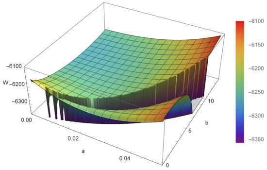
Figure 6. The real part of the effective potential $W_{gl}^{SU\left(2\right)}$ (167), as a function of the $A_0$-background a and the magnetic background b (see Equation (168)) for $T=10$ and $g=1$.

After submitting this review, a continuation of the above investigation appeared [69]. There, it is shown that at high temperature, a minimum in both $A_0$ and B exists in a region with no imaginary part.

6. Concluding Remarks

In the foregoing sections, we reviewed instabilities that arise in magnetic background fields either from the coupling of fields with spin $s\ge 1$ with the background or from radiative corrections (or from a combination of them). Thereby, we tried to provide an approach to the topic that was readable with a generic background in QFT. In general, QFT, and the SM especially, are the foundation of our understanding of the world. A huge amount of methods and calculations are known and are in excellent agreement with experiments, using the anomalous magnetic moment of the electron as one example. Thereby, the perturbative approach plays an essential role. However, with the tachyonic instabilities, which appear in the perturbative approach, there are two phenomena that lack real understanding. Both are related to the tachyonic modes that appear from the coupling of the magnetic moment of a one-spin field to a magnetic background field in a non-Abelian gauge theory.

In the EW theory, it is the W-boson that may have a tachyonic mode. However, due to its mass, this instability appears only for very strong magnetic fields. Thus, it will show up at best in cosmology. It is a common belief that in such fields, a condensation of W-bosons should happen. However, this topic is not worked out in sufficient detail.

In QCD, the gluon field is massless, and the instability is immanently present (at least at low energy and temperature). In a first approach, this instability resulted in the Savvidy vacuum, which is, however, not stable. Despite numerous attempts and approaches, this problem is unsolved along with the confinement problem. We also review an approach with background fields, having an $A_0$ field and a magnetic component. This approach, however, has raised more questions. The present review may inspire further research in these directions. After submitting this review, two new papers, Refs. [54,69], appeared, which together with [50], give the topic of color magnetic background fields a new dynamic.

References

- Huang, K. Quarks, Leptons & Gauge Fields, 2nd ed.; World Scientific: Singapore, 1992. [Google Scholar]
- Schwinger, J. On Quantum-Electrodynamics and the Magnetic Moment of the Electron. Phys. Rev. 1948, 73, 416–417. [Google Scholar] [CrossRef]
- Ryder, L.H. Quantum Field Theory; Cambridge University Press: Cambridge, UK, 1985. [Google Scholar]
- Vasiliev, A. Functional Methods in Quantum Field Theory and Statistical Physics; Gordon and Breach: Philadelphia, PA, USA, 1998. [Google Scholar]
- Kirsten, K. Spectral Functions in Mathematics and Physics; Chapman&Hall/CRC: Boca Raton, FL, USA, 2001. [Google Scholar]
- Vassilevich, D. Heat kernel expansion: User’s manual. Phys. Rept. 2003, 388, 279–360. [Google Scholar] [CrossRef]
- Bordag, M.; Klimchitskaya, G.L.; Mohideen, U.; Mostepanenko, V.M. Advances in the Casimir Effect; Oxford University Press: Oxford, UK, 2009. [Google Scholar]
- Coleman, S.; Weinberg, E. Radiative Corrections as the Origin of Spontaneous Symmetry Breaking. Phys. Rev. D 1973, 7, 1888–1910. [Google Scholar] [CrossRef]
- Heisenberg, W.; Euler, H. Consequences of Dirac’s theory of positrons. Z. Phys. 1936, 98, 714–732. [Google Scholar] [CrossRef]
- Schwinger, J. On gauge invariance and vacuum polarization. Phys. Rev. D 1951, 8, 664–679. [Google Scholar] [CrossRef]
- Savvidy, G. Infrared Instability of Vacuum State of Gauge Theories and Asymptotic Freedom. Phys. Lett. B 1977, 71, 133–134. [Google Scholar] [CrossRef]
- Nielsen, N.; Olesen, P. Unstable Yang-Mills Field Mode. Nucl. Phys. B 1978, 144, 376–396. [Google Scholar] [CrossRef]
- Gornicki, P.; Mankiewicz, L.; Zembowicz, R. On Spontaneous Pair Creation. J. Phys. A Math. Gen. 1987, 20, 6593–6596. [Google Scholar] [CrossRef]
- O’Connell, R.F. Effect of the Anomalous Magnetic Moment of the Electron on Spontaneous Pair Production in a Strong Magnetic Field. Phys. Rev. Lett. 1968, 21, 397–398. [Google Scholar] [CrossRef]
- Jancovici, B. Radiative Correction to the Ground-State Energy of an Electron in an Intense Magnetic Field. Phys. Rev. 1969, 187, 2275. [Google Scholar] [CrossRef]
- Demeur, M. Etude de l’interaction entre le champ propre d’une particule et un champ electro-magnetique homogene et constant. Mem. Acad. Roy. Belg. Cl. Sci. Bruxelles 1953, 28, 98. [Google Scholar]
- Ternov, I.; Bagrov, V.; Bordovitsin, V.; Dorofeev, O. Concerning Anomalous Magnetic Moment of Electron. Sov. Phys. Jetp-Ussr 1969, 28, 1206. [Google Scholar]
- Tsai, W.; Yildiz, A. Motion of an Electron in a Homogeneous Magnetic-Field-Modified Propagation Function and Synchrotron Radiation. Phys. Rev. D 1973, 8, 3446–3460. [Google Scholar] [CrossRef]
- Baier, V.; Katkov, V.; Strakhovenko, V. Anomalous Magnetic-Moment of an Electron in a Magnetic-Field. Sov. J. Nucl. Phys. 1976, 24, 197–199. [Google Scholar] [CrossRef]
- Tsai, W.Y. Modified electron propagation function in strong magnetic fields. Phys. Rev. D 1974, 10, 1342–1345. [Google Scholar] [CrossRef]
- Baier, V.; Baier, V.; Strakhovenko, V. Structure of Electron Mass Operator in a Homogeneous Magnetic-Field close to the Critical Strength. Sov. Phys. JETP 1990, 71, 657–666. [Google Scholar]
- Linde, A. Phase-Transitions In Gauge-Theories And Cosmology. Rep. Prog. Phys. 1979, 42, 389–437. [Google Scholar] [CrossRef]
- Amelino-Camelia, G.; Pi, S.Y. Self-consistent improvement of the finite-temperature effective potential. Phys. Rev. D 1993, 47, 2356–2362. [Google Scholar] [CrossRef]
- Pilaftsis, A.; Teresi, D. Symmetry-improved CJT effective action. Nucl. Phys. B 2013, 874, 594–619. [Google Scholar] [CrossRef]
- Sher, M. Electroweak Higgs potential and vacuum stability. Phys. Rep. 1989, 179, 273–418. [Google Scholar] [CrossRef]
- Arnold, P. Phase transition temperatures at next-to-leading order. Phys. Rev. D 1992, 46, 2628–2635. [Google Scholar] [CrossRef]
- Ekstedt, A.; Löfgren, J. A critical look at the electroweak phase transition. J. High Energy Phys. 2020, 2020, 136. [Google Scholar] [CrossRef]
- Midorikawa, S. Symmetry restoration of the electroweak interactions. Phys. Rev. D 1980, 22, 2045–2053. [Google Scholar] [CrossRef]
- Skalozub, V. Nonabelian Gauge-Theories in an External Electromagnetic-Field. Sov. J. Nucl. Phys. 1980, 31, 412–416. [Google Scholar]
- Shore, G.M. Symmetry restoration and the background field method in gauge theories. Ann. Phys. 1981, 137, 262–305. [Google Scholar] [CrossRef]
- Ghoroku, K. Structure of the Effective Potential under a Constant Magnetic Field for SU(2) Yang-Mills Theory. Prog. Theor. Phys. 1982, 68, 1340–1353. [Google Scholar] [CrossRef]
- Skalozub, V. Abrikosov Lattice in the Theory of Electroweak Interactions. Sov. J. Nucl. Phys. 1986, 43, 665–669. [Google Scholar]
- Salam, A.; Strathdee, J. Transition electromagnetic fields in particle physics. Nucl. Phys. B 1975, 90, 203–220. [Google Scholar] [CrossRef]
- Skalozub, V. On the Restoration of Spontaneously Broken Symmetry in a Magnetic Field. Sov. J. Nucl. Phys. 1978, 28, 113–115. [Google Scholar]
- Skalozub, V. Vacuum of the electroweak interactions in strong external fields. Sov. J. Part. Nucl. 1985, 16, 445. [Google Scholar]
- Skalozub, V.; Vanyashin, V. Study of W-Boson in a Magnetic-Field Based Upon Both Mass Operator and Effective Potential. Fortschr. Phys. 1992, 40, 739–760. [Google Scholar] [CrossRef]
- Kirzhnits, D.; Linde, A. Macroscopic consequences of the Weinberg model. Phys. Lett. B 1972, 42, 471–474. [Google Scholar] [CrossRef]
- Weinberg, S. Gauge and global symmetries at high temperature. Phys. Rev. D 1974, 9, 3357–3378. [Google Scholar] [CrossRef]
- Cabo, A.; Kalashnikov, O.; Shabad, A. Finite Temperature Gluonic Gas in a Magnetic-Field. Nucl. Phys. B 1981, 185, 473. [Google Scholar] [CrossRef]
- Dittrich, W.; Schanbacher, V. The effective QCD lagrangian at finite temperature. Phys. Lett. B 1981, 100, 415–419. [Google Scholar] [CrossRef]
- Nielsen, H.; Olesen, P. A quantum liquid model for the QCD vacuum: Gauge and rotational invariance of domained and quantized homogeneous color fields. Nucl. Phys. B 1979, 160, 380–396. [Google Scholar] [CrossRef]
- Arodz, H.; Zalewski, K. Remark on the Copenhagen Vacuum. Acta Phys. Polon. 1981, B12, 115. [Google Scholar]
- Skalozub, V. Condensation of Magnetic Vortex Lines in Yang-Mills Theory. Sov. J. Nucl. Phys. 1985, 41, 1044–1048. [Google Scholar]
- Ambjørn, J.; Olesen, P. Anti-screening of large magnetic fields by vector bosons. Phys. Lett. B 1988, 214, 565–569. [Google Scholar] [CrossRef]
- Ambjørn, J.; Olesen, P. On electroweak magnetism. Nucl. Phys. B 1989, 315, 606–614. [Google Scholar] [CrossRef]
- Ambjørn, J.; Olesen, P. Electroweak Magnetism—Theory And Applications. Int. J. Mod. Phys. A 1990, 5, 4525–4557. [Google Scholar] [CrossRef]
- Nielsen, H.; Ninomiya, M. A bound on bag constant and Nielsen-Olesen unstable mode in QCD. Nucl. Phys. B 1979, 156, 1–28. [Google Scholar] [CrossRef]
- Nielsen, N.; Olesen, P. Electric vortex lines from the Yang-Mills theory. Phys. Lett. B 1978, 79, 304–308. [Google Scholar] [CrossRef]
- Cabo Montes de Oca, A.; Manreza Paret, D.; Pérez Martínez, A.; Rodriguez Querts, E.; Piccineli, G. On the instabiity of the SM for magnetic fields larger than M2W/e. Astron. Nachrichten 2015, 336, 845–850. [Google Scholar] [CrossRef]
- Bordag, M. Tachyon condensation in a chromomagnetic background field and the groundstate of QCD. Eur. Phys. J. A 2023, 59, 55. [Google Scholar] [CrossRef]
- Leutwyler, H. Constant Gauge Fields and their Quantum Fluctuations. Nucl. Phys. 1981, B179, 129–170. [Google Scholar] [CrossRef]
- Consoli, M.; Preparata, G. On the stability of the perturbative ground state in non-abelian Yang-Mills theories. Phys. Lett. B 1985, 154, 411–417. [Google Scholar] [CrossRef]
- Maiani, L.; Martinelli, G.; Rossi, G.; Testa, M. A constant chromomagnetic field leads nowhere. Nucl. Phys. B 1986, 273, 275–296. [Google Scholar] [CrossRef]
- Savvidy, G. Stability of Yang Mills vacuum state. Nucl. Phys. B 2023, 990, 116187. [Google Scholar] [CrossRef]
- Flory, C.A. Covariant Constant Chromomagnetic Fields and Elimination of the One Loop Instabilities. 1983. SLAC-PUB3244, Preprint. Available online: https://lib-extopc.kek.jp/preprints/PDF/1983/8312/8312331.pdf (accessed on 16 March 2023).
- Nielsen, H.; Olesen, P. Vortex-line models for dual strings. Nucl. Phys. B 1973, 61, 45–61. [Google Scholar] [CrossRef]
- Achúcarro, A.; Vachaspati, T. Semilocal and electroweak strings. Phys. Rep. 2000, 327, 347–426. [Google Scholar] [CrossRef]
- Hindmarsh, M. Existence and stability of semilocal strings. Phys. Rev. Lett. 1992, 68, 1263–1266. [Google Scholar] [CrossRef]
- James, M.; Perivolaropoulos, L.; Vachaspati, T. Detailed stability analysis of electroweak strings. Nucl. Phys. B 1993, 395, 534–546. [Google Scholar] [CrossRef]
- Weigel, H.; Quandt, M.; Graham, N. Quantum stabilization of cosmic strings. Mod. Phys. Lett. A 2015, 30, 1530022. [Google Scholar] [CrossRef]
- Bordag, M.; Drozdov, I. Fermionic vacuum energy from a Nielsen-Olesen vortex. Phys. Rev. 2003, D68, 065026. [Google Scholar] [CrossRef]
- Diakonov, D.; Maul, M. Center-vortex solutions of the Yang-Mills effective action in three and four dimensions. Phys. Rev. D 2002, 66, 096004. [Google Scholar] [CrossRef]
- Bordag, M. Vacuum energy of a color magnetic vortex. Phys. Rev. 2003, D67, 065001. [Google Scholar] [CrossRef]
- Skalozub, V.; Chub, I. 2-Loop Contribution of Quarks to the Condensate of the Gluon Field at Finite Temperatures. Phys. At. Nucl. 1994, 57, 324. [Google Scholar]
- Korthals Altes, C.P.; Nishimura, H.; Pisarski, R.D.; Skokov, V.V. Free energy of a holonomous plasma. Phys. Rev. D 2020, 101, 094025. [Google Scholar] [CrossRef]
- Skalozub, V.V. Nielsen’s identity and gluon condensation at finite temperature. Phys. Rev. D 1994, 50, 1150–1156. [Google Scholar] [CrossRef]
- Ebert, D.; Zhukovsky, V.C.; Vshivtsev, A.S. Thermodynamic potential with condensate fields in an SU(2) model of QCD. Int. J. Mod. Phys. 1998, A13, 1723–1742. [Google Scholar] [CrossRef]
- Bordag, M.; Skalozub, V. Effective potential of gluodynamics in background of Polyakov loop and colormagnetic field. Eur. Phys. J. C 2022, 82, 390. [Google Scholar] [CrossRef]
- Skalozub, V. Spontaneous magnetization of a vacuum in high temperature gluodynamics (two-loop approximation). arXiv 2023, arXiv:2305.00757. [Google Scholar]
- Newton, R.G. Radiative Effects in a Constant Field. Phys. Rev. 1954, 96, 523–528. [Google Scholar] [CrossRef]
Disclaimer/Publisher’s Note: The statements, opinions and data contained in all publications are solely those of the individual author(s) and contributor(s) and not of MDPI and/or the editor(s). MDPI and/or the editor(s) disclaim responsibility for any injury to people or property resulting from any ideas, methods, instructions or products referred to in the content. |
© 2023 by the author. Licensee MDPI, Basel, Switzerland. This article is an open access article distributed under the terms and conditions of the Creative Commons Attribution (CC BY) license (https://creativecommons.org/licenses/by/4.0/).