Abstract
The motion of photons and the frequency shift of photons emitted by particles orbiting the central black hole described by the deformed Reissner–Nordström spacetime metric is investigated. It has been shown that in spacetime, two stable photon spheres are formed due to the gravitational attraction of photons by the central gravitating compact object. It has been found that as spacetime parameters increase, charge and deformation photon spheres become smaller in size and the effect of the electric charge is stronger than the effect of the deformation parameter. The frequency shift of photons radiated by the particles at the equatorial plane becomes stronger for the smaller values of the deformation parameter and the electric charge of the deformed Reissner–Nordström black hole.
Keywords:
black holes; general relativity; modified gravity; photon motion; frequency shift of photons; Hubble Law PACS:
04.20.−q; 04.50.+h; 04.70.−s; 04.70.Bw; 04.50.−h
1. Introduction
General relativity (GR), proposed by Albert Einstein as a metric theory of gravitational interaction, has been well-tested in regimes consisting of weak (using a solar system test, gravitational lensing, etc. [1,2]) and strong (using gravitational waves and black hole (BH) observations [3,4,5,6,7,8,9,10,11,12,13,14,15]). The nonlinear field equations of GR determine the metric of curved spacetime resulting from the gravitational field. The first solutions describing spherically symmetric solutions of Einstein’s equations were obtained by Schwarzschild in 1916 [16]. Another black hole solution in the framework of GR was derived by Reissner and Nordström in 1918 [17,18] describing a charged, non-rotating BH. However, these solutions have a fundamental problem related to the physical singularity at the origin of the point-like source. This issue cannot be eliminated within classical field theory and one has to think beyond the standard frames. Various astrophysical phenomena associated with black holes containing electric charge, generalizations of these solutions, and observational constraints on the charge of black hole candidates can be found enough in the literature. We wish to highlight some of the following valuable works: [19,20,21,22,23].
One of the approaches to eliminate the singularity at the center is to couple the GR with nonlinear electrodynamics [24,25,26,27,28]. Due to the effects of nonlinear electric and/or magnetic charges, the radial coordinate in the metric function will be modified, and does not contain the singularity.
Another fundamental issue of GR is related to the explanation of the nature and behavior of the so-called dark matter and dark energy. Plenty of alternative models can explain the new forms of matter using, say, additional scalar, vector, and tensor fields. These modifications may explain the effects of dark matter and dark energy not predicted by standard cosmology. At the same time, developers of these modifications believe that they can resolve the singularity problem of GR.
However, many proposed modified and alternative theories of gravity create another issue related to degeneracy, and mimic the effects due to various parameters of different solutions. One way to resolve this issue is to use parametrization of the spacetime metric. The deflection from the standard spherical symmetric solution of GR can be expressed in terms of a series of small expansion parameters [29,30,31,32]. This approach was proposed by Johannsen and Psaltis [30] and was further developed and analyzed by various authors, e.g., [33,34,35,36,37,38,39,40].
Testing the general theory of relativity (GR) and other gravity theories using observational data constitutes a primary objective within the realm of contemporary relativistic astrophysics. The recent groundbreaking discoveries of gravitational waves [3,4,5,6,7] and the imaging of supermassive BHs M87* and Sgr A* [8,9,10,11,12,13,14,15] have opened up opportunities to develop new tests for gravity theories in the strong field regime. In particular, the optical, radiative, and energetic properties of several BH solutions, with the aim of developing new probes of the gravity models, have been explored in Refs. [41,42,43,44].
In this paper, we present our findings on photon motion around a deformed (extended) Reissner–Nordström black hole (RN BH). We use the analysis of gravitational lensing and light deflection caused by gravitationally compact objects to test gravity models. In this study, our objective is to expand the examination of photon movement around a deformed Reissner–Nordström black hole (DRN BH) and thoroughly explore the impact of gravitational redshift. The structure of the paper is as follows: Section 2 delves into the characteristics of the spacetime surrounding the deformed RN BH. In Section 3, we analyze the trajectory of photons on the equatorial plane. The investigation of the redshift and blueshift phenomena experienced by emitted photons is carried out in Section 4 using detectors in circular orbits. In Section 5, we consider the detector to be radially moving with respect to the black hole and apply the results to the Hubble law. Section 6 provides a concise overview of the primary findings obtained in this paper. Throughout the study, we adopt geometrized units with , utilize Greek indices ranging from 0 to 3, and consider the spacetime signature as (−,+,+,+).
2. Deformed Reissner–Nordström Black Hole Solution
In the literature, there are numerous analytical solutions for various gravitational field equations. In order to facilitate the comparison and potential astrophysical applications, several parametrizations were suggested. For example, the line element of the general spacetime around a deformed RN BH can be expressed [30,45]
where M represents the total mass of the central BH, and Q is the electric charge. The radial function
is expressed as an infinite series in terms of small dimensionless perturbation parameters . According to the Johannsen–Psaltis parameterization, the known spacetimes—being exact analytical solutions of the gravitational field equations—are extended in the dimensionless parameter . The Johannsen–Psaltis spacetime metric is an approximate representation of the Einstein equations, presented as a power series in , with coefficients depending on the matter fields. However, it is closely aligned with what we might expect as solutions of modified gravity equations. The constraints obtained using data from the lunar laser ranging experiment [46] have shown that and are negligibly small and vanish. The lowest-order nonvanishing parameter is usually taken into account in astrophysical scenarios. In particular, this parameter is called the deformation parameter due to the change in the spacetime structure in the presence of . It is also worth noting that positive and negative values of the deformation parameter correspond to oblate or prolate deformations, respectively [30]. The analysis of the lapse function (1), in terms of radial coordinates, is shown in Figure 1 for different values of the deformation parameter and electric charge of the black hole. From these dependencies, one may easily see that, in large distances, the spacetime turns to the Minkowski one. In the left panel of Figure 1, it is evident that larger values of the electric charge parameter lead to a reduction in the values of the lapse function in the immediate vicinity of the central compact object. The right panel of Figure 1 presents an opposite effect that can be observed, i.e., the increase in the deformation parameter increases the lapse function near the central black hole. However, at large distances, the effects of the spacetime parameters become negligible.
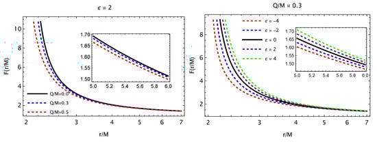
Figure 1.
The variation of the lapse function with respect to the radial distance around the deformed RN BH. In the figure, is given as . In the left panel, the deformation parameter is fixed as , and the different curves are responsible for the selected values of the BH charge. In the right panel, the BH charge is fixed as , and the different curves are responsible for the selected values of the deformation parameter.
The event horizon location can be found from condition . This equation can be written in the following form:
The solution of this equation gives the radius of the event’s horizon, which is the same as for the RN BH, and can be written as follows:
One can see that the given spacetime describes a black hole when has two horizons, i.e., inner (−) and outer (+) ones. One can also easily notice that the effect of the deformation parameter on the event horizon is absent and, thus, this solution coincides with the event horizon radius of RN BH. This is because the term containing the deformation parameter appears to be in the denominator of the expression (4).
Thermodynamics
We will now calculate the entropy and temperature of the black hole described by the spacetime metric (1). The event horizon of the black hole can be defined using condition ; consequently, one may define the area of the event horizon of black hole A as
Accordingly, the Bekenstein–Hawking entropy reads as follows:
The Hawking temperature can be expressed as [47,48]
where and are metric components and prime () denotes the derivative with respect to r, and the expression of is given as
Figure 2 displays the correlation between the temperature and spacetime parameters. The right panel of the figure indicates that the deformation parameter has a minimal (almost negligible) effect on the temperature (T) of the black hole, which slightly decreases as the parameter value increases. Conversely, the left panel indicates that the temperature experiences a significant decrease when the electric charge value rises.
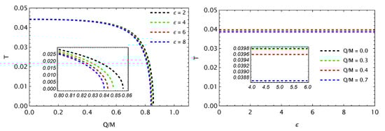
Figure 2.
Variation of temperature with the horizon radius for the different values of parameter and .
We can calculate one of the thermodynamics variables, specifically the Gibbs energy. To determine the Gibbs energy, we will use the following equation:
where H is the enthalpy of the black hole. In general, by using the equivalence of mass M and enthalpy H, we can write the following: M = H.
Now, we obtain the expression for the Gibbs free energy by substituting Equations (7) and (8) into Equation (10), as
The first panel in Figure 3 depicts the relationship between the Gibbs free energy and the BH charge for various values of the deformation parameter . It is evident that the Gibbs free energy experiences a minor increase with a rising electric charge. By examining the left panel of Figure 3, it is apparent that the Gibbs free energy varies slowly as the value of the deformation parameter increases, as apparent from the right panel.
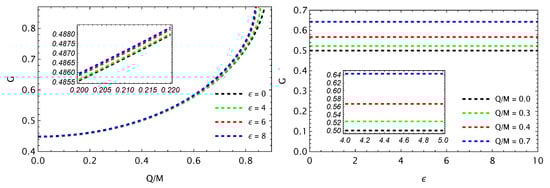
Figure 3.
Variation of the Gibbs free energy with the horizon radius for different values of parameter and .
3. Photon Motion
It is convenient to use Hamilton–Jacobi formalism to investigate the motion of photons within the spacetime surrounding deformed RN BH, which can be expressed as
where the action can be expressed in the following form:
due to the symmetries of the spacetime metric tensor. The conserved quantities, and , may be referred to as the energy of the photon and its angular momentum. At the equatorial plane (), the effective potential of a photon simplifies its motion:
Figure 4 illustrates the radial dependence of the effective potential governing the radial motion of photons across various values of the spacetime parameters. The left panel of Figure 4 clearly demonstrates that larger values of the electric charge parameter result in a reduced effective potential for photons in the vicinity of a central black hole. However, at larger distances, the influence of the magnetic charge becomes negligible. From the right panel of Figure 4, one can see that the opposite behavior of the effective potential took place, i.e., the increase in the deformation parameter made the effective potential bigger. One can also clearly see that the effect of the deformation parameter was considerably stronger than the magnetic charge.
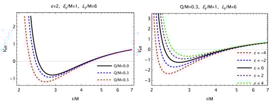
Figure 4.
The influence of the electric charge (left) and the deformation parameter (right) on the radial behavior of the effective potential for photons in the vicinity of a deformed RN black hole is demonstrated.
The unstable circular orbits or so-called photon sphere radius can be defined using the following conditions
with the prime symbol () denoting the derivative with respect to r. By solving the set of Equations (15) and (16), one can establish a relationship between the photon sphere radius and parameters of the given spacetime. This relationship is depicted for the metric given by (1) in Figure 5. The solid lines in Figure 5 correspond to the event horizon radius. Observing the left panel of Figure 5, it is evident that an increase in the electric charge leads to a reduction in the photon sphere radius. This effect is akin to the change observed in the event horizon radius (represented by the black solid line). When the electric charge assumes a non-zero value, two horizons emerge, i.e., an inner horizon and an outer horizon. These horizons merge into one at the extreme value of electric charge . Beyond the extreme value, the presence of a naked singularity is encountered. Furthermore, from the left panel of Figure 5, it can be observed that, starting from electric charge values around , and when , two lines corresponding to the photon sphere radius appear (upper and lower green dashed lines), with the second line being very close to the event horizon. To test the stability of orbits, one can examine the sign of . It has been found that both lines correspond to stable orbits, as indicated by . Hence, it can be concluded that in the presence of deformation, a black hole can possess two photon spheres when the electric charge exceeds a specific threshold. Additionally, it is worth noting that for larger values of , the lines shift toward smaller radii.
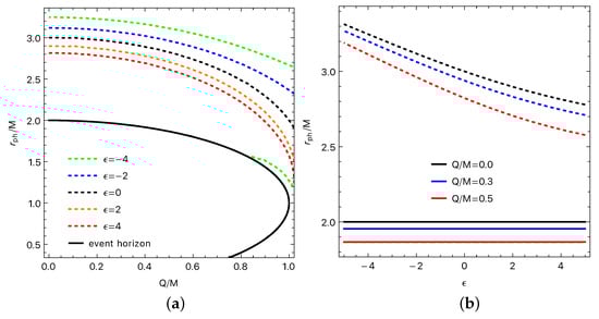
Figure 5.
The variation of the photon sphere radius with respect to the spacetime parameters Q and is depicted (solid lines). The solid lines in the figure represent the event horizon radius of a black hole. Subfigure (a) shows that increase of the electric charge reduces the photon sphere radius and the event horizon radius. Subfigure (b) reveals that increase of the deformation parameter affects the photon sphere radius only not changing event horizon radius. Further information can be found in the main text.
Conversely, the influence of on the photon sphere radius is more direct. The right panel of Figure 5 clearly illustrates that, for fixed values of the black hole’s electric charge Q, the photon sphere always exists above the event horizon radius within the specified range of . Additionally, it is important to note that the event horizon is solely influenced by the electric charge Q and remains independent of the deformation parameter .
4. Gravitational Redshift of Photons for Circularly Orbiting Detector
In this section, we analyze the red/blueshift phenomena of photons radiated by particles in motion around a deformed RN BH using the Herrera–Nucamendi (HN) algorithm described in Ref. [49]. The frequency shift z can be defined as
Here, represents the frequency observed by an observer in motion with the photon emitter particle, while corresponds to the frequency observed by an observer located far away from the emission source. One may express the frequencies and in the following form
In the given context, can be considered as the four-velocity of a particle following a geodesic path, while denotes the four-momentum of photons traveling along null geodesics, which satisfy the condition .
In order to find the expressions for and , Euler–Lagrange equations can be employed:
where Lagrangian can be defined as
In this case, , where represents the proper time. The presence of space-like and time-like killing vectors enables the derivation of conserved quantities, namely, the energy E and angular momentum L, which correspond to the symmetries associated with the t and coordinates, respectively.
Equations (21) and (22) can be utilized to express the t and components of the four-velocity in the following manner:
The normalization condition can be rewritten as
or in the form
where the effective potential of radial motion is defined as
Using the Lagrangian (20), one can easily analyze the four-momentum for photons. The energy and the component of the angular momentum orthogonal to the azimuthal rotation, which are conserved quantities, take the forms
The expression for ,which is defined in Equation (18), can be now rewritten as
or
The observational data can be analyzed in relation to a kinematic frequency shift, denoted as . This shift is defined as the difference between the observed redshift z and the central frequency shift . The central frequency shift corresponds to the gravitational frequency shift experienced by a photon emitted from a static particle positioned along the line connecting the center of coordinates to the distant observer. Consequently, one may have
One may also rewrite the expression in the following form:
where is interpreted as the apparent impact parameter. We should note that when and remain conserved along null trajectories from the emission point to the point of detection, holds true.
Furthermore, we will use for analysis. In particular, in the equatorial plane () Equation (32) can be rewritten as
Equation (33) does not incorporate the light bending effect caused by the gravitational field. To incorporate this effect, we determine the impact parameter , where represents the radius of the circular orbit of the photon emitter. Additionally, we consider photons emitted from both sides of the compact object, with the conditions and . Note that and are expressed by (28). Taking into account condition , it is easy to obtain the following:
When the observer is located very far from the source (), one may have and . Consequently, Equation (33) can be rewritten as
Different signs of and in Equation (34) correspond to the redshift () and blueshift ().
The effective potential in the equatorial plane takes the following form:
In the case of circular orbits, both and become zero. Such conditions enable us to derive and , which are applicable to any static, spherically symmetric spacetime. These expressions can be written as follows:
For the stability of circular orbits, one needs to consider an additional condition, i.e., . Equations (37) and (38) allow us to express as
Using (23), we can easily derive the four-velocity expression in the following form:
The angular velocity of particles in circular orbits will take the following form:
The explicit expressions for and can be used to find the frequency shift as follows:
Now, we can examine the red/blueshifts of light emitted by geodesic particles moving along circular trajectories with a radius of . To simplify the analysis, we will consider only the positive sign of the frequency shift (redshift), as in the spherically symmetric spacetime, the redshift and blueshift of photons differ from each other only in sign.
By utilizing the spacetime described by Equation (1) and employing Equation (42), one can derive the radial dependence of the frequency shift of photons for various values of the electric charge and deformation parameter of the deformed RN BH, as illustrated in Figure 6. The left panel demonstrates a weak dependency of the frequency shift on the electric charge of the black hole, with a slight reduction as the charge increases. In contrast, the right panel of Figure 6 reveals a relatively stronger influence of the deformation parameter on the frequency shift compared to the effect of the electric charge parameter. Additionally, it can be observed that an increase in the deformation parameter leads to a smaller frequency shift of photons. It is worth noting that, for both cases, the effects of the electric charge and the deformation parameter become negligible at larger distances.
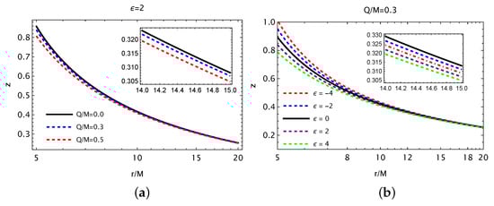
Figure 6.
Variation of the redshift of photons with radial coordinates for different values of the electric charge (a) and deformation parameter (b) of RN BH.
The dependence of the redshift factor on the BH parameters is shown in Figure 7. It is evident from the upper left panel that the redshift exhibits larger values at smaller distances, and for a smaller electric charge parameter, as indicated by the red region in the plot. The upper right panel illustrates a similar trend, where larger values of z correspond to smaller values of . In the bottom panel, the relationship between the frequency shift of photons and the spacetime parameters is depicted for a fixed radial distance from the central black hole. It is now apparent that smaller values of the deformation parameter and electric charge parameter result in a stronger shift in the frequency of photons emitted by geodesic particles moving in the equatorial plane of the central black hole.
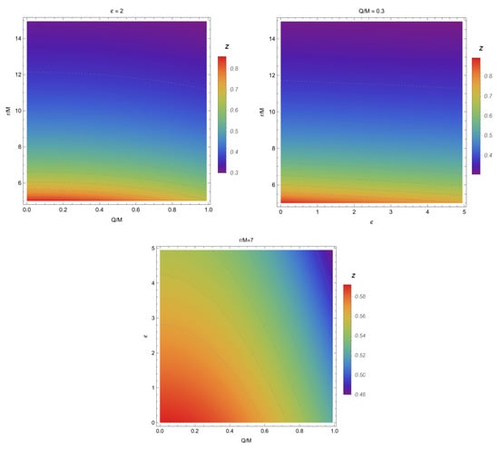
Figure 7.
The relationship between the redshift of photons and the radial coordinate, as well as the spacetime parameters of the deformed RN BH.
5. Radially Moving Detector and the Hubble Law
The effect of dark energy is dominant for the large distances measured in megaparsecs. In this case, in the spacetime metric, one needs to take into account the term involving the cosmological constant. Since the cosmological part is responsible for the background effects, one may neglect the effect of the black hole solution. In this case, the line element of the spacetime around the deformed RN BH with cosmological constant can be expressed as
We will now focus on analyzing the redshift of the deformed RN BH, denoted as , in terms of the spacetime parameters. Specifically, we consider a special configuration involving circularly orbiting emitters and the radial motion of detectors. From this setup, we extract the Hubble law based on certain physical approximations.
Due to the accelerated expansion of the Universe, attributed to the positive cosmological constant at larger scales, the detector is expected to move away from the black hole. This is particularly relevant for our study, as we are interested in far-away detectors. Therefore, in this case, we examine a detector that moves radially away from the deformed RN BH, deviating from the usual circular orbit or static detector configurations.
By employing this particular configuration, we can express the frequency shift of photons (29) as follows:
In order to calculate Equation (44), one needs to know the four-velocity expressions of emitters in equatorial motion and detectors in radial motion, in terms of the black hole parameters. In previous sections, from condition , we already found the non-vanishing components, and , of the emitter in the equatorial plane, , , and . Consequently, one can write and in the following form:
On the other hand, for the detector that radially moves away from the deformed RN BH, the conditions should be and . As a result, using , the non-vanishing components of the detector read as follows:
From condition , one may easily find the radial component of the four-momentum of photons. Consequently, the ratio can be expressed as
where the quantity is given as
In Equation (47), the ‘+’ and ‘−’ signs of b correspond to the redshift and blueshift photons, respectively.
Now, substituting , and from Equations (45)–(48) into Equation (44), one can obtain the final expressions for the redshift and blueshift of the deformed RN BH. Finally, the redshift expression can be expressed as
where
where is the radius of the emitter and is the distance between the black hole and the detector.
It is important to note that, in real astrophysical systems, such as supermassive black holes in water vapor clouds (referred to as megamasers), the emitter radius is typically on a sub-parsec scale ( pc), while the detector radius needs to be on a much larger scale of tens of mega-parsecs to account for the Hubble flow ( Mpc). Moreover, the mass and charge of black holes are of the same order as the event horizon radius, , and the cosmological constant is of the order m [50]. Therefore, considering a configuration that involves a supermassive black hole with a mass approximately equivalent to solar masses in the Hubble flow, we can estimate , , , and . These estimations lead to the following implications
Thus, one may neglect the following terms , keeping the dominant terms for tracking the general relativistic effects. Now, Equation (49) takes the form
where is the contribution of the cosmological constant in the redshift. The Hubble constant is related to the cosmological constant with [50]
where is the cosmological constant density parameter. When (this case corresponds to the Universe filled with dark energy), one may recover the Hubble law as as
where is the velocity of the host galaxy going away from the detector, represents the distance between the black hole and the observer. Now, Equation (52) will take the form
where is the frequency shift of the deformed RN BH and is the frequency of the Schwarzschild black holes.
Please note that Equation (55) cannot be regarded as a simple multiplication of and by hand. The second factor in this equation arises naturally as a dominant term in the cosmological redshift due to considerations from general relativity. The most general and intricate expressions are derived from the roots of Equations (49) and (50). This formula indicates that when photons emitted by massive geodesic particles—orbiting a dRN black hole—reach the detector, they carry information about the mass M, electric charge Q, deformation , and cosmological constant . This information is encoded in the frequency shift of these photons, denoted as in Equation (55), which is directly observable. Consequently, by performing a statistical fit [49,51,52,53] or solving an inverse problem, as demonstrated in [54], the set of spacetime parameters can be estimated. In other words, Equation (55) enables the extraction of the spacetime properties characterized by the black hole mass M, electric charge Q, deformation , and cosmological constant through the measurement of frequency shifts in the photons, .
We may now determine , taking the limit , , and in Equation (49), as follows
since the term is neglected and we keep the first dominant term . Now, one may expand Equation (56) to and .
with and it should be noted that the upper(lower) sign refers to blueshift (redshift) photons. Equations (55) and (57) can be used to obtain
with and . Proceeding to the next step, we solve the initial Equation (58) in order to obtain the mass of the Schwarzschild black hole, yielding the following result
in terms of the frequency shift and product. It is important to mention that if the constant is set to zero, we obtain the mass formula in terms of R and B derived in [54]. To determine the relationship between the term and the redshift, we substitute Equation (60) into Equation (59) and solve as follows:
Equation (61) provides the Hubble constant expressed in relation to the frequency shift R and B of photons located on opposite sides of the RN black hole, along with the distance between the detector and the black hole, denoted as . As a result, the product that appears in Equation (61) can be utilized to express the mass relation (60) solely in terms of the blueshift and redshift. On the other hand, from Equation (59), we can straightforwardly derive the following expression:
to derive the mass parameter solely based on the observational quantities R and B.
In the case where , a special situation arises where we have (as indicated in Equation (59)). Under this circumstance, the redshift and blueshift become nearly equal, denoted as . Consequently, by taking the limit , we can derive Hubble’s law for this specific case from the analytical expression in Equation (62), yielding the following result
6. Conclusions
In our study, we opted for a model where the deformed RN BH solution represents the spacetime surrounding a central compact object. Our investigation focused on studying the motion of photons and analyzing the resulting frequency shift. We discovered that the formation of a photon sphere around the central black hole is significantly influenced by two spacetime parameters: the electric charge of the black hole and the deformation parameter of the central black hole. Furthermore, we established that the event horizon radius is exclusively sensitive to the electric charge, while the photon sphere radius is affected by both spacetime parameters. Interestingly, we demonstrated the existence of two stable photon spheres that intersect at specific values of these two spacetime parameters. Additionally, our findings indicate that an increase in the electric charge parameter leads to a reduction in the size of the photon sphere. Moreover, we have shown that the influence of the electric charge of the central black hole on the photon sphere radius is more pronounced compared to the effect of the deformation parameter.
By examining the frequency shift of photons observed by a circularly moving detector, we discovered that the influence of spacetime parameters on this quantity is minimal at large distances, but becomes significant in the immediate vicinity of the central black hole. Our findings indicate that the frequency shift of photons is more pronounced for lower values of the electric charge associated with the central black hole. Similarly, we observed a similar effect when considering the dependence of the frequency shift of photons on the deformation parameter of the central compact object. The last density plots provided a more informative visualization of these results, further validating our findings.
In our research, we provided a demonstration of the frequency shift experienced by photons emitted by massive objects, such as stars, which are in circular orbits around KdS black holes. We investigated how this frequency shift is influenced by various spacetime parameters, including the mass of the black hole, its electric charge, the deformation parameter, and the cosmological constant. To accomplish this, we considered detectors in radial motion relative to the emitter-black hole system and employed a general relativistic framework, as briefly outlined in the text.
Furthermore, our observations revealed that the frequency shift of photons increases with an augmentation in the cosmological constant and the distance between the detector and the emitter-black hole system. These findings align with the repulsive nature typically associated with the cosmological constant. Consequently, we derived the Hubble law based on the initial redshift equations, incorporating certain physically plausible approximations.
Additionally, we obtained analytical equations for the mass of the Schwarzschild black hole and the Hubble constant to the frequency shifts exhibited by massive objects moving in circular orbits around the static, spherically symmetric black hole. Notably, we made an intriguing discovery regarding the natural emergence of the Hubble law, which is derived from the precise formulation of the Hubble constant presented in Equation (61). These remarkable formulas, discovered through our research, offer a concise and elegant approach to extracting valuable information about the properties of spacetime, including the black hole’s mass, spin, and cosmological constant, by simply measuring the frequency shift of photons.
Author Contributions
Writing—original draft, H.A., B.N., A.A. and B.A.; Writing—review and editing, B.N. and B.A.; investigation, H.A. and B.N.; supervision, B.N., A.A. and B.A. All authors have read and agreed to the published version of the manuscript.
Funding
This research was funded by Ministry of Innovative Development of the Republic of Uzbekistan: Grants F-FA-2021-510, F-FA-2021-432, and MRB-2021-527.
Data Availability Statement
Not applicable.
Acknowledgments
The research presented in this study is funded by grants F-FA-2021-510, F-FA-2021-432, and MRB-2021-527 from the Ministry for Innovative Development of Uzbekistan. A.A. would like to acknowledge the support of the PIFI fund from the Chinese Academy of Sciences.
Conflicts of Interest
The authors declare no conflict of interest.
References
- Ni, W.T. Solar-system tests of the relativistic gravity. Int. J. Mod. Phys. D 2016, 25, 1630003. [Google Scholar] [CrossRef]
- Treschman, K. Recent astronomical tests of general relativity. Int. J. Phys. Sci. 2015, 10, 90–105. [Google Scholar] [CrossRef]
- Abbott, B.P.; Abbott, R.; Abbott, T.D.; Acernese, F.; Ackley, K.; Adams, C.; Adams, T.; Addesso, P.; Adhikari, R.X.; Adya, V.B.; et al. GW170104: Observation of a 50-Solar-Mass Binary Black Hole Coalescence at Redshift 0.2. Phys. Rev. Lett. 2017, 118, 221101, Erratum in Phys. Rev. Lett. 2018, 121, 129901. [Google Scholar] [CrossRef] [PubMed]
- Abbott, B.P.; Abbott, R.; Abbott, T.D.; Abernathy, M.R.; Acernese, F.; Ackley, K.; Adams, C.; Adams, T.; Addesso, P.; Adhikari, R.X.; et al. Binary Black Hole Mergers in the first Advanced LIGO Observing Run. Phys. Rev. X 2016, 6, 041015, Erratum in Phys. Rev. X 2018, 8, 039903. [Google Scholar] [CrossRef]
- Abbott, B.P.; Abbott, R.; Abbott, T.D.; Abernathy, M.R.; Acernese, F.; Ackley, K.; Adams, C.; Adams, T.; Addesso, P.; Adhikari, R.X.; et al. GW151226: Observation of Gravitational Waves from a 22-Solar-Mass Binary Black Hole Coalescence. Phys. Rev. Lett. 2016, 116, 241103. [Google Scholar] [CrossRef]
- Abbott, B.P.; Abbott, R.; Abbott, T.D.; Abernathy, M.R.; Acernese, F.; Ackley, K.; Adams, C.; Adams, T.; Addesso, P.; Adhikari, R.X.; et al. Tests of general relativity with GW150914. Phys. Rev. Lett. 2016, 116, 221101, Erratum in Phys. Rev. Lett. 2018, 121, 129902. [Google Scholar] [CrossRef]
- Abbott, B.P.; Abbott, R.; Abbott, T.D.; Abernathy, M.R.; Acernese, F.; Ackley, K.; Adams, C.; Adams, T.; Addesso, P.; Adhikari, R.X.; et al. Observation of Gravitational Waves from a Binary Black Hole Merger. Phys. Rev. Lett. 2016, 116, 061102. [Google Scholar] [CrossRef]
- Akiyama, K.; Alberdi, A.; Alef, W.; Asada, K.; Azulay, R.; Baczko, A.-K.; Ball, D.; Baloković, M.; Barrett, J.; Bintley, D.; et al. First M87 Event Horizon Telescope Results. I. The Shadow of the Supermassive Black Hole. Astrophys. J. 2019, 875, L1. [Google Scholar] [CrossRef]
- Akiyama, K.; Alberdi, A.; Alef, W.; Asada, K.; Azulay, R.; Baczko, A.-K.; Ball, D.; Baloković, M.; Barrett, J.; Bintley, D.; et al. First M87 Event Horizon Telescope Results. II. Array and Instrumentation. Astrophys. J. Lett. 2019, 875, L2. [Google Scholar] [CrossRef]
- Akiyama, K.; Alberdi, A.; Alef, W.; Asada, K.; Azulay, R.; Baczko, A.-K.; Ball, D.; Baloković, M.; Barrett, J.; Bintley, D.; et al. First M87 Event Horizon Telescope Results. III. Data Processing and Calibration. Astrophys. J. Lett. 2019, 875, L3. [Google Scholar] [CrossRef]
- Akiyama, K.; Alberdi, A.; Alef, W.; Asada, K.; Azulay, R.; Baczko, A.-K.; Ball, D.; Baloković, M.; Barrett, J.; Bintley, D.; et al. First M87 Event Horizon Telescope Results. IV. Imaging the Central Supermassive Black Hole. Astrophys. J. Lett. 2019, 875, L4. [Google Scholar] [CrossRef]
- Akiyama, K.; Alberdi, A.; Alef, W.; Asada, K.; Azulay, R.; Baczko, A.-K.; Ball, D.; Baloković, M.; Barrett, J.; Bintley, D.; et al. First M87 Event Horizon Telescope Results. V. Physical Origin of the Asymmetric Ring. Astrophys. J. Lett. 2019, 875, L5. [Google Scholar] [CrossRef]
- Akiyama, K.; Alberdi, A.; Alef, W.; Algaba, J.C.; Anantua, R.; Asada, K.; Azulay, R.; Bach, U.; Baczko, A.-K.; Ball, D.; et al. First Sagittarius A* Event Horizon Telescope Results. I. The Shadow of the Supermassive Black Hole in the Center of the Milky Way. Astrophys. J. Lett. 2022, 930, L12. [Google Scholar] [CrossRef]
- Akiyama, K.; Alberdi, A.; Alef, W.; Algaba, J.C.; Anantua, R.; Asada, K.; Azulay, R.; Bach, U.; Baczko, A.-K.; Ball, D.; et al. First Sagittarius A* Event Horizon Telescope Results. III. Imaging of the Galactic Center Supermassive Black Hole. Astrophys. J. Lett. 2022, 930, L14. [Google Scholar] [CrossRef]
- Akiyama, K.; Alberdi, A.; Alef, W.; Algaba, J.C.; Anantua, R.; Asada, K.; Azulay, R.; Bach, U.; Baczko, A.-K.; Ball, D.; et al. First Sagittarius A* Event Horizon Telescope Results. VI. Testing the Black Hole Metric. Astrophys. J. Lett. 2022, 930, L17. [Google Scholar] [CrossRef]
- Schwarzschild, K. On the gravitational field of a mass point according to Einstein’s theory. Sitzungsber. Preuss. Akad. Wiss. Berlin (Math. Phys.) 1916, 1916, 189–196. [Google Scholar]
- Reissner, H. Über die Eigengravitation des elektrischen Feldes nach der Einsteinschen Theorie. Annalen der Physik 1916, 355, 106–120. [Google Scholar] [CrossRef]
- Nordström, G. On the Energy of the Gravitation field in Einstein’s Theory. K. Ned. Akad. Van Wet. Proc. Ser. Phys. Sci. 1918, 20, 1238–1245. [Google Scholar]
- Turimov, B.; Alibekov, H.; Tadjimuratov, P.; Abdujabbarov, A. Gravitational synchrotron radiation and Penrose process in STVG theory. Phys. Lett. B 2023, 843, 138040. [Google Scholar] [CrossRef]
- Zakharov, A. New Astron. 10, 479 (2005); AF Zakharov, F. De Paolis, G. Ingrosso, and AA Nucita. Astron. Astrophys. 2005, 442, 795. [Google Scholar] [CrossRef]
- Zakharov, A.F. Constraints on tidal charge of the supermassive black hole at the Galactic Center with trajectories of bright stars. Eur. Phys. J. C 2018, 78, 689. [Google Scholar] [CrossRef] [PubMed]
- Prokopov, V.; Alexeyev, S. Shadow from a rotating black hole in an extended gravity. Int. J. Mod. Phys. A 2020, 35, 2040060. [Google Scholar] [CrossRef]
- Alexeyev, S.O.; Latosh, B.N.; Prokopov, V.A.; Emtsova, E.D. Phenomenological Extension for Tidal Charge Black Hole. J. Exp. Theor. Phys. 2019, 128, 720–726. [Google Scholar] [CrossRef]
- Bardeen, J. In Proceedings of the GR5; DeWitt, C., DeWitt, B., Eds.; USSR, Gordon and Breach: Tbilisi, Georgia, 1968; p. 174. [Google Scholar]
- Ayón-Beato, E.; García, A. Regular Black Hole in General Relativity Coupled to Nonlinear Electrodynamics. Phys. Rev. Lett. 1998, 80, 5056–5059. [Google Scholar] [CrossRef]
- Ayon-Beato, E.; Garcia, A. New regular black hole solution from nonlinear electrodynamics. Phys. Lett. B 1999, 464, 25. [Google Scholar] [CrossRef]
- Wang, A.; Maartens, R. Cosmological perturbations in Horava-Lifshitz theory without detailed balance. Phys. Rev. D 2010, 81, 024009. [Google Scholar] [CrossRef]
- Toshmatov, B.; Stuchlík, Z.; Schee, J.; Ahmedov, B. Electromagnetic perturbations of black holes in general relativity coupled to nonlinear electrodynamics. Phys. Rev. D 2018, 97, 084058. [Google Scholar] [CrossRef]
- Johannsen, T.; Psaltis, D. Testing the No-Hair Theorem with Observations in the Electromagnetic Spectrum: I. Properties of a Quasi-Kerr Spacetime. Astrophys. J. 2010, 716, 187–197. [Google Scholar] [CrossRef]
- Johannsen, T.; Psaltis, D. Metric for rapidly spinning black holes suitable for strong-field tests of the no-hair theorem. Phys. Rev. D 2011, 83, 124015. [Google Scholar] [CrossRef]
- Rezzolla, L.; Zhidenko, A. New parametrization for spherically symmetric black holes in metric theories of gravity. Phys. Rev. D 2014, 90, 084009. [Google Scholar] [CrossRef]
- Yunes, N.; Pretorius, F. Fundamental theoretical bias in gravitational wave astrophysics and the parametrized post-Einsteinian framework. Phys. Rev. D 2009, 80, 122003. [Google Scholar] [CrossRef]
- Atamurotov, F.; Abdujabbarov, A.; Ahmedov, B. Shadow of rotating non-Kerr black hole. Phys. Rev. D 2013, 88, 064004. [Google Scholar] [CrossRef]
- Hakimov, A.; Atamurotov, F. Gravitational lensing by a non-Schwarzschild black hole in a plasma. Astrophys. Space Sci. 2016, 361, 112. [Google Scholar] [CrossRef]
- Rayimbaev, J.; Turimov, B.; Marcos, F.; Palvanov, S.; Rakhmatov, A. Particle acceleration and electromagnetic field of deformed neutron stars. Mod. Phys. Lett. A 2019, 35, 2050056. [Google Scholar] [CrossRef]
- Liu, C.; Chen, S.; Jing, J. Rotating non-Kerr black hole and energy extraction. Astrophys. J. 2012, 751, 148. [Google Scholar] [CrossRef]
- Jiang, J.; Bambi, C.; Steiner, J.F. Using iron line reverberation and spectroscopy to distinguish Kerr and non-Kerr black holes. J. Cosmol. Astropart. Phys. 2015, 5, 025. [Google Scholar] [CrossRef]
- Liu, D.; Li, Z.; Bambi, C. Testing a class of non-Kerr metrics with hot spots orbiting SgrA*. J. Cosmol. Astropart. Phys. 2015, 1, 020. [Google Scholar] [CrossRef]
- Bambi, C. Measuring the Kerr spin parameter of a non-Kerr compact object with the continuum-fitting and the iron line methods. J. Cosmol. Astropart. Phys. 2013, 8, 055. [Google Scholar] [CrossRef]
- Bambi, C. A code to compute the emission of thin accretion disks in non-Kerr space-times and test the nature of black hole candidates. Astrophys. J. 2012, 761, 174. [Google Scholar] [CrossRef]
- Rayimbaev, J.; Narzilloev, B.; Abdujabbarov, A.; Ahmedov, B. Dynamics of Magnetized and Magnetically Charged Particles around Regular Nonminimal Magnetic Black Holes. Galaxies 2021, 9, 71. [Google Scholar] [CrossRef]
- Narzilloev, B.; Rayimbaev, J.; Abdujabbarov, A.; Ahmedov, B. Regular Bardeen Black Holes in Anti-de Sitter Spacetime versus Kerr Black Holes through Particle Dynamics. Galaxies 2021, 9, 63. [Google Scholar] [CrossRef]
- Narzilloev, B.; Hussain, I.; Abdujabbarov, A.; Ahmedov, B.; Bambi, C. Dynamics and fundamental frequencies of test particles orbiting Kerr–Newman–NUT–Kiselev black hole in Rastall gravity. Eur. Phys. J. Plus 2021, 136, 1032. [Google Scholar] [CrossRef]
- Narzilloev, B.; Hussain, I.; Abdujabbarov, A.; Ahmedov, B. Optical properties of an axially symmetric black hole in the Rastall gravity. Eur. Phys. J. Plus 2022, 137, 645. [Google Scholar] [CrossRef]
- Rahim, R.; Saifullah, K. Charging the Johannsen—Psaltis spacetime. Ann. Phys. 2019, 405, 220–233. [Google Scholar] [CrossRef]
- Will, C.M. The Confrontation between General Relativity and Experiment. Living Rev. Rel. 2014, 17, 4. [Google Scholar] [CrossRef]
- Hawking, S.W. Black hole explosions. Nature 1974, 248, 30–31. [Google Scholar] [CrossRef]
- Banerjee, R.; Ranjan Majhi, B. Quantum tunneling beyond semiclassical approximation. J. High Energy Phys. 2008, 2008, 095. [Google Scholar] [CrossRef]
- Nucamendi, U.; Herrera-Aguilar, A.; Lizardo-Castro, R.; Cruz, O.L. Toward the Gravitational Redshift Detection in NGC 4258 and the Estimation of Its Black Hole Mass-to-distance Ratio. Astrophys. J. Lett. 2021, 917, L14. [Google Scholar] [CrossRef]
- Carroll, S.M. The Cosmological constant. Living Rev. Rel. 2001, 4, 1. [Google Scholar] [CrossRef]
- Villalobos-Ramirez, A.; Gallardo-Rivera, O.; Herrera-Aguilar, A.; Nucamendi, U. A general relativistic estimation of the black hole mass-to-distance ratio at the core of TXS 2226–184. Astron. Astrophys. 2022, 662, L9. [Google Scholar] [CrossRef]
- Villaraos, D.; Herrera-Aguilar, A.; Nucamendi, U.; González-Juárez, G.; Lizardo-Castro, R. A general relativistic mass-to-distance ratio for a set of megamaser AGN black holes. Mon. Not. R. Astron. Soc. 2022, 517, 4213–4219. [Google Scholar] [CrossRef]
- Villalobos-Ramírez, A.; González-Juárez, A.; Momennia, M.; Herrera-Aguilar, A. A general relativistic mass-to-distance ratio for a set of megamaser AGN black holes II. arXiv 2022, arXiv:2211.06486. [Google Scholar]
- Banerjee, P.; Herrera-Aguilar, A.; Momennia, M.; Nucamendi, U. Mass and spin of Kerr black holes in terms of observational quantities: The dragging effect on the redshift. Phys. Rev. D 2022, 105, 124037. [Google Scholar] [CrossRef]


Disclaimer/Publisher’s Note: The statements, opinions and data contained in all publications are solely those of the individual author(s) and contributor(s) and not of MDPI and/or the editor(s). MDPI and/or the editor(s) disclaim responsibility for any injury to people or property resulting from any ideas, methods, instructions or products referred to in the content. |
© 2023 by the authors. Licensee MDPI, Basel, Switzerland. This article is an open access article distributed under the terms and conditions of the Creative Commons Attribution (CC BY) license (https://creativecommons.org/licenses/by/4.0/).