Dynamics in a Competitive Nicholson’s Blowflies Model with Continuous Time Delays

Abstract

In this study, we examine a competitive Nicholson blowflies model with time-varying coefficients and continuous time delays. In the case of coincidence degree theory, constructing appropriate Lyapunov functionals and using several inequalities, several conditions on the extinction, periodic solution, permanence, and global attractiveness of the system are derived. Finally, three examples with numerical simulations are presented to validate the practicability and feasibility of the obtained theoretical results.

1. Introduction

In recent decades, with the continuous development of population dynamics, the theory of the Nicholson’s blowflies model has made significant progress. The Nicholson’s blowflies model is a mathematical model used to study the population dynamics of blowflies. In addition, this model is to understand and explain the observed patterns and fluctuations in blowfly populations. By developing a mathematical model, researchers aim to gain insights into the mechanisms governing population growth, population decline, and the factors influencing blowfly populations. One of the most interesting aspects of Nicholson’s blowflies model is its dynamic behavior. Recently, the dynamic behavior of a series of special Nicholson’s blowflies models was investigated. For example, to describe the development law of Nicholson’s blowflies and better comply with Nicholson’s empirical data [1], Gurney established a discrete time-delayed Nicholson’s blowflies model with constant coefficients and linear death density for the first time

$$\dot{S}\left(t\right)=-\varrho S\left(t\right)+\rho S(t-\theta ){\mathrm{e}}^{-\alpha S(t-\theta )}.$$

(1)

Based on model (1), in [2], Saker established a discrete time-delayed Nicholson’s blowflies model with time-varying coefficients and linear death density

$$\begin{array}{c}\hfill \dot{S}\left(t\right)=-\varrho \left(t\right)S\left(t\right)+\rho \left(t\right)S(t-m\theta ){\mathrm{e}}^{-\alpha S(t-m\theta )},\end{array}$$

(2)

and certain criteria for the existence and global attractiveness of positive periodic solutions of system (2) were obtained. Subsequently, based on models (1) and (2), Berezansky [3] studied a delayed Nicholson’s blowflies model with constant coefficients and nonlinear death density and obtained some new research results. At the same time, several open problems were proposed. In [4], the following delayed autonomous model is studied

$$\begin{array}{c}{\dot{S}}_1\left(t\right)=-a_1{S}_1\left(t\right)+b_1{S}_2\left(t\right)+c_1{S}_1(t-\gamma ){\mathrm{e}}^{-S_1(t-\gamma )},\hfill \\ {\dot{S}}_2\left(t\right)=-a_2{S}_2\left(t\right)+b_2{S}_1\left(t\right)+c_2{S}_2(t-\gamma ){\mathrm{e}}^{-S_2(t-\gamma )}.\hfill \end{array}$$

(3)

The existence and uniqueness conditions, uniform persistence conditions, and local and global convergence conditions of the equilibrium solution of the model (3) were obtained. In addition, the above Nicholson’s blowflies model assumes constant population growth rates and reproduction rates. However, in real-world scenarios, population and reproduction rates might change periodically due to seasonal variations or other factors. By incorporating temporal symmetries, such as periodicity or oscillations, into the model, one can analyze how blowfly populations might fluctuate over time. For example, in [5], the authors studied a Nicholson-type system with continuous time delays

$$\begin{array}{ll}{\dot{S}}_1\left(t\right)=& -{\alpha }_1\left(t\right)S_1\left(t\right)+{\beta }_1\left(t\right)S_2\left(t\right)+c_1\left(t\right)S_1\left(t-{\varpi }_1\left(t\right)\right)e^{-{\delta }_1\left(t\right)S_1\left(t-{\varpi }_1\left(t\right)\right)}\\ & -H_1\left(t\right)S_1\left(t-{\varpi }_1\left(t\right)\right),\\ {\dot{S}}_2\left(t\right)=& -{\alpha }_2\left(t\right)S_2\left(t\right)+{\beta }_2\left(t\right)S_1\left(t\right)+c_2\left(t\right)S_2\left(t-{\varpi }_2\left(t\right)\right)e^{-{\delta }_2\left(t\right)S_2\left(t-{\varpi }_2\left(t\right)\right)}\\ & -H_2\left(t\right)S_2\left(t-{\varpi }_2\left(t\right)\right),\end{array}$$

(4)

and the criteria for the global existence and uniqueness of periodic solution of the system were obtained.

It can be found that the various groups in model (3) and model (4) considered in [4,5] have cooperative relationships. However, competition between biological populations is often more likely to occur. In addition, as people continue to deepen the process of revealing natural laws, the research on competitive multipopulation Nicholson’s blowflies systems with time delays often enables us to more objectively understand the true laws of the development of biological populations in the real world, which will also contribute to further improving and developing the theory and application of functional differential equations and biological population dynamics. Therefore, it is of great significance to study the dynamics of various types of Nicholson’s blowflies delay systems such as competitive Nicholson’s blowflies systems with delays [6]. However, there are few studies on the multipopulation Nicholson’s blowflies model of the competitive type. For example, in [6], the authors established a delayed competitive Nicholson’s blowflies model with constant coefficients for the first time.

$$\begin{array}{c}{\dot{y}}_1\left(t\right)=-\delta y_1\left(t\right)+a{y}_1\left(t-{\varsigma }_1\right){\mathrm{e}}^{-b{y}_1\left(t-{\varsigma }_1\right)}-k_1{y}_1\left(t\right)y_2\left(t\right),\hfill \\ {\dot{y}}_2\left(t\right)=-\delta y_2\left(t\right)+a{y}_2\left(t-{\varsigma }_2\right){\mathrm{e}}^{-b{y}_2\left(t-{\varsigma }_2\right)}-k_2{y}_1\left(t\right)y_2\left(t\right).\hfill \end{array}$$

(5)

Some results on the stability and attractiveness of equilibrium points were obtained for system (5). It can be found that system (5) and the considered systems in [7,8] are autonomous, and the time delays are discrete. However, in the real world, nonautonomous variable time-delayed differential equations can better reflect the real ecosystem situation. Therefore, we need to introduce variable delay into nonautonomous models. There has been some studies [9,10,11,12,13,14,15] related to the study of Nicholson’s blowflies models with continuous time delays.

To further understand how blowfly populations respond to various factors, such as temperature, food availability, and competition, and to aid in the development of effective pest management strategies and provide valuable information for ecological research, in this study, we extended system (5) to the time-varying coefficients and continuous time delayed case, and we investigated the following competitive Nicholson’s blowflies model with time-varying coefficients and continuous time delays

$$\begin{array}{c}{\dot{x}}_1\left(t\right)=-\delta \left(t\right)x_1\left(t\right)+a\left(t\right)x_1\left(t-{\gamma }_1\left(t\right)\right){\mathrm{e}}^{-b\left(t\right)x_1\left(t-{\gamma }_1\left(t\right)\right)}-k_1\left(t\right)x_1\left(t\right)x_2\left(t\right),\hfill \\ {\dot{x}}_2\left(t\right)=-\delta \left(t\right)x_2\left(t\right)+a\left(t\right)x_2\left(t-{\gamma }_2\left(t\right)\right){\mathrm{e}}^{-b\left(t\right)x_2\left(t-{\gamma }_2\left(t\right)\right)}-k_2\left(t\right)x_1\left(t\right)x_2\left(t\right),\hfill \end{array}$$

(6)

where $x_i\left(t\right)(i=1,2)$ represents the number of organisms in the two regions at time t, $a\left(t\right)$ represents the maximum daily reproduction rate of adult individuals, $\frac{1}{b\left(t\right)}$ represents the number of organisms bred at the maximum reproduction rate at time t, $\delta \left(t\right)$ represents the daily average mortality rate of adult individuals at time t, ${\gamma }_1\left(t\right)$, ${\gamma }_2\left(t\right)$ represent the time from birth to adulthood, and $k_1\left(t\right)$ and $k_2\left(t\right)$ represent the proportional coefficient of death caused by mutual aggression due to compete resources at t. Compared with previous research results, the nonautonomous competitive Nicholson’s blowflies model (6) that we considered has not been studied so far. Next, we study the permanence, extinction, the existence of positive periodic solutions, and the sufficient conditions for the global attractivity of model (6).

For system (6), we use the following initial conditions:

$$\begin{array}{c}\hfill x_i\left(t\right)={\varphi }_i\left(t\right)(i=1,2),t\in [-\xi ,0],\end{array}$$

(7)

${\varphi }_i\left(t\right)(i=1,2)$ is a non-negative continuous function defined on $[-\xi ,0]$ that satisfies ${\varphi }_i\left(0\right)>0(i=1,2)$, where $\xi ={\max }_{t\in [0,+\infty )}\{{\gamma }_i\left(t\right),(i=1,2)\}.$

For system (6), we have the following assumptions:

$\left({\mathbf{H}}_1\right)$$k_1\left(t\right)>0, k_2\left(t\right)>0, {\gamma }_1\left(t\right)>0, {\gamma }_2\left(t\right)>0, \delta \left(t\right)>0$ and $a\left(t\right)>0, b\left(t\right)>0$ are all continuous bounded functions on $[0,+\infty )$.

$\left({\mathbf{H}}_2\right)$$k_1\left(t\right)>0, k_2\left(t\right)>0, {\gamma }_1\left(t\right)>0, {\gamma }_2\left(t\right)>0, \delta \left(t\right)>0$ and $a\left(t\right)>0, b\left(t\right)>0$ are all continuous bounded and $\Omega$-periodic functions on $[0,+\infty )$.

Now, we give a notation and three important lemmas to be used in this paper. In this paper, we define

$$\begin{array}{c}{\mathrm{Y}}^L={\displaystyle \underset{t\in [0,+\infty )}{{\displaystyle \inf }}}\mathrm{Y}\left(t\right),{\mathrm{Y}}^M=\underset{t\in [0,+\infty )}{\sup }\mathrm{Y}\left(t\right),\overline{F}=\frac{1}{\Omega }{\int }_0^{\Omega }F\left(t\right)dt,\end{array}$$

where $\mathrm{Y}\left(t\right)$ is a any bounded continuous function defined on $[0,+\infty )$, and $\mathrm{Y}\left(t\right)$ is any $\Omega$-periodic continuous function on $[0,+\infty )$.

Lemma 1

([3]). Consider the following equation

$$\begin{array}{c}\hfill \dot{N}\left(t\right)=-\delta N\left(t\right)+P\sum _{k=1}^m{a}_k\left(t\right)N\left(h_k\left(t\right)\right){\mathrm{e}}^{-N\left(h_k\left(t\right)\right)},t\ge t_0,\end{array}$$

where $\delta >0,P>0$ are non-negative constants, $a_k\left(t\right)\ge 0(k=1,2,\cdots ,m)$, and $h_k\left(t\right):[0,\infty )\to \mathbb{R}(k=1,2,\cdots ,m)$ is the Lebesgue measurable function that satisfies ${\sum }_{k=1}^m{a}_k\left(t\right)=1,h_k\left(t\right)\le t, {\lim }_{t\to \infty }{h}_k\left(t\right)=\infty$. If $P>\delta {\mathrm{e}}^2$, then

$$\underset{t\to \infty }{\lim }\sup N\left(t\right)\le \frac{P}{\delta \mathrm{e}},\underset{t\to \infty }{\lim }\inf N\left(t\right)\ge \frac{P^2}{{\delta }^2\mathrm{e}}{\mathrm{e}}^{-\frac{P}{{\delta }_e}}.$$

Lemma 2

([7]). Consider equation $\dot{S}\left(t\right)=pS(t-\upsilon )-qS\left(t\right)$, where $p>0,q>0,\upsilon >0$, when $S\left(t\right)>0$ for $t\in [-\upsilon ,0]$, we have:

(1) 

If $p<q$, then ${\lim }_{t\to +\infty }S\left(t\right)=0$;

(2) 

If $p>q$, then ${\lim }_{t\to +\infty }S\left(t\right)=+\infty$.

The organization of this paper as follows: In the next section, findings from the research study are presented. In Section 3, three examples are given to illustrate that our main results are applicable. Finally, in Section 4, the main findings and key points of the research are summarized, and the scope of future work is presented.

2. Main Results

In this section, we obtain some sufficient conditions on the boundedness, permanence, extinction, periodic solution, and global attractivity of system (6).

Theorem 1.

Suppose that $\left({\mathbf{H}}_1\right)$ holds and

$$a^L>({\delta }^M+\frac{a^M}{\mathrm{e}{b}^L{\delta }^L}k)b^M{\mathrm{e}}^2,$$

(8)

where $k=\max \left\{k_1^M,k_2^M\right\}$, then system (6) is permanent.

We need the following two lemmas to prove Theorem 1.

Lemma 3.

Suppose that $\left({\mathbf{H}}_1\right)$ holds, then there is a positive number $M>0$ such that

$$\underset{t\to \infty }{\lim }\sup x_i\left(t\right)\le M,$$

for any positive solution $x_i\left(t\right)(i=1,2)$ of system (6).

Proof. 

First, it can be obtained from system (6) for $i=1,2$ and $t\ge \xi$ that

$${\dot{x}}_i\left(t\right)\le -{\delta }^L{x}_i\left(t\right)+\frac{a^M}{b^L}{b}^L{x}_i\left(t-{\gamma }_i\left(t\right)\right){\mathrm{e}}^{-b^L{x}_i\left(t-{\gamma }_i\left(t\right)\right)}.$$

(9)

Consider the following auxiliary equation

$${\dot{u}}_i\left(t\right)=-{\delta }^L{u}_i\left(t\right)+\frac{a^M}{b^L}{b}^L{u}_i\left(t-{\gamma }_i\left(t\right)\right){\mathrm{e}}^{-b^L{u}_i\left(t-{\gamma }_i\left(t\right)\right)}.$$

From Lemma 1, we can obtain

$$\underset{t\to +\infty }{\lim }\sup x_i\left(t\right)\le \frac{a^M}{e{\delta }^L{b}^L}:=M.$$

(10)

Therefore, there is a positive number $T_1$, such that $x_i\left(t\right)\le M$ for $t>T_1$. This completes the proof. □

Lemma 4.

Suppose that $\left({\mathbf{H}}_1\right)$ and inequality (8) hold, then there are positive numbers $m_i>0$$(i=1,2)$ such that

$$\underset{t\to \infty }{\lim }\inf x_i\left(t\right)\ge m_i,$$

for any positive solution $x_i\left(t\right)(i=1,2)$ of system (6).

Proof. 

From system (6) for $i=1,2$ and $t>T_1$, we can obtain

$${\dot{x}}_i\left(t\right)\ge \frac{a^L}{b^M}{b}^M{x}_i\left(t-{\gamma }_i\left(t\right)\right){\mathrm{e}}^{-b^M{x}_i\left(t-{\gamma }_i\left(t\right)\right)}-\left({\delta }^M+M{k}_i^M\right)x_i\left(t\right).$$

(11)

Consider auxiliary equation

$${\dot{u}}_i\left(t\right)=\frac{a^L}{b^M}{b}^M{u}_i\left(t-{\gamma }_i\left(t\right)\right){\mathrm{e}}^{-b^M{u}_i\left(t-{\gamma }_i\left(t\right)\right)}-A_i{u}_i\left(t\right),$$

where $A_i={\delta }^M+M{k}_i^M$. From Lemma 1, we obtain

$$\underset{t\to +\infty }{\mathrm{lim\; inf}} u_i\left(t\right)\ge \frac{{\left(a^L\right)}^2}{A_i^2{\left(b^M\right)}^{2}e}{\mathrm{e}}^{-\frac{a^L}{A_i{b}^{M}e}}.$$

So, we have

$$\underset{t\to +\infty }{\mathrm{lim\; inf}} x_i\left(t\right)\ge \frac{{\left(a^L\right)}^2}{A_i^2{\left(b^M\right)}^2\mathrm{e}}{\mathrm{e}}^{-\frac{a^L}{A_i{b}^{M}e}}:=m_i,i=1,2.$$

(12)

 □

From Lemmas 3 and 4, we can obtain the permanence of system (6).

Corollary 1.

If $\left({\mathbf{H}}_2\right)$ and condition (8) hold, then system (6) is permanent.

From Lemma 2, we have the following result:

Lemma 5.

Suppose that $\left({\mathbf{H}}_1\right)$ holds and ${\delta }^L>a^M$, then system (6) is extinct.

Proof. 

First, when $t\ge \xi$, $i=1,2$, for system (6), we have

$${\dot{x}}_i\left(t\right)\le -{\delta }^L{x}_i\left(t\right)+a^M{x}_i\left(t-{\gamma }_i\left(t\right)\right).$$

(13)

Consider auxiliary equation

$${\dot{u}}_i\left(t\right)=-{\delta }^L{u}_i\left(t\right)+a^M{u}_i\left(t-{\gamma }_i\left(t\right)\right),$$

From Lemma 2, we can obtain

$$\underset{t\to +\infty }{\lim }{u}_i\left(t\right)=0,i=1,2.$$

(14)

Therefore, we have positive number $T_2$, such that $x_i\left(t\right)\to 0(i=1,2)$ for $t>T_2$. □

Theorem 2.

Suppose that $\left({\mathbf{H}}_2\right)$ holds and $D_0>1$, then system (6) has a positive Ω-periodic solution, where $D_0=\min \{{\inf }_{t\in R}\frac{a\left(t\right)}{\delta \left(t\right)},{\inf }_{t\in R}\frac{\delta \left(t\right)}{k\left(t\right)}\}$, $k\left(t\right)=\max \{k_1\left(t\right),k_2\left(t\right)\}$.

Proof. 

Let

$$x_1\left(t\right)=e^{u_1\left(t\right)},x_2\left(t\right)=e^{u_2\left(t\right)}.$$

(15)

Then, we obtain

$$\begin{array}{c}\hfill {\dot{u}}_1\left(t\right)=-\delta \left(t\right)+\frac{a\left(t\right)e^{u_1(t-{\gamma }_1\left(t\right))}}{e^{b\left(t\right)e^{u_1(t-{\gamma }_1\left(t\right))}+u_1\left(t\right)}}-k_1\left(t\right)e^{u_2\left(t\right)}:={\Delta }_1(u,t),\\ \hfill {\dot{u}}_2\left(t\right)=-\delta \left(t\right)+\frac{a\left(t\right)e^{u_2(t-{\gamma }_2\left(t\right))}}{e^{b\left(t\right)e^{u_2(t-{\gamma }_2\left(t\right))}+u_2\left(t\right)}}-k_2\left(t\right)e^{u_1\left(t\right)}:={\Delta }_2(u,t).\end{array}$$

(16)

We find that if system (16) has an $\Omega$-periodic solution ${(u_1^{*}\left(t\right),u_2^{*}\left(t\right))}^T$, then ${\left(x_1^{*}\left(t\right),x_2^{*}\left(t\right)\right)}^T$$={\left(e^{u_1\left(t\right)},e^{u_2\left(t\right)}\right)}^T$ is the positive $\Omega$-periodic solution of system (6). Now, we only need to prove that system (16) has an $\Omega$-periodic solution. From continuation theorem [16], we define the normed vector spaces $\mathcal{X}$ and $\mathcal{Z}$. Let

$$\mathcal{X}=\mathcal{Z}=\left\{u={\left(u_1\left(\kappa \right),u_2\left(\kappa \right)\right)}^T\in C\left(R,R^2\right):u(\kappa +\Omega )=u\left(\kappa \right),\kappa \in R\right\},$$

be a Banach space with norm $\parallel ·\parallel$. For any $u\in \mathcal{X}$, we find that $\Delta (u,·)$ $={\left({\Delta }_1(u,·),{\Delta }_2(u,·)\right)}^T$$\in C\left(R,R^2\right)$ is an $\Omega$-periodic solution. Let

$$\begin{array}{cc}\hfill \mathcal{L}:\mathcal{D}\left(\mathcal{L}\right)=\{u\in \mathcal{X}:& \left.u\in C^1\left(R^1,R^2\right)\right\}\ni u⟼\dot{u}={\left({\dot{u}}_1,{\dot{u}}_2\right)}^T\in \mathcal{Z},\hfill \\ \hfill \mathcal{P}:\mathcal{X}\ni u& ⟼{\left(\frac{1}{\Omega }{\int }_0^{\Omega }{u}_1\left(s\right)ds,\frac{1}{\Omega }{\int }_0^{\Omega }{u}_2\left(s\right)ds\right)}^T\in \mathcal{X},\hfill \\ \hfill \mathcal{Q}:\mathcal{Z}\ni z& ⟼{\left(\frac{1}{\Omega }{\int }_0^{\Omega }{z}_1\left(s\right)ds,\frac{1}{\Omega }{\int }_0^{\Omega }{z}_2\left(s\right)ds\right)}^T\in \mathcal{Z},\hfill \\ & \mathcal{N}:\mathcal{X}\ni u⟼\Delta (u,·)\in \mathcal{Z}.\hfill \end{array}$$

It is easy to see that

$$Im\mathcal{L}=\left\{u\mid u\in \mathcal{Z},{\int }_0^{\Omega }u\left(s\right)ds={(0,0)}^T\right\},Ker\mathcal{L}=R^2,$$

$$Im\mathcal{P}=Ker\mathcal{L}\mathrm{and}Ker\mathcal{Q}=Im\mathcal{L}.$$

Therefore, $\mathcal{L}$ is a Fredholm operator with zero index. In addition, defining ${\mathcal{L}}_{\mathcal{P}}^{-1}:Im\mathcal{L}\to \mathcal{D}\left(\mathcal{L}\right)\cap Ker\mathcal{P}$ as the reciprocal of ${\left.\mathcal{L}\right|}_{\mathcal{D}\left(\mathcal{L}\right)\cap Ker\mathcal{P}}$, we obtain

$$\begin{array}{ll}{\mathcal{L}}_{\mathcal{P}}^{-1}y\left(t\right)& =-\frac{1}{\Omega }{\int }_0^{\Omega }{\int }_0^{t}y\left(s\right)dsdt+{\int }_0^{t}y\left(s\right)ds\\ & ={\left(-\frac{1}{\Omega }{\int }_0^{\Omega }{\int }_0^t{y}_1\left(s\right)dsdt+{\int }_0^t{y}_1\left(s\right)ds,-\frac{1}{\Omega }{\int }_0^{\Omega }{\int }_0^t{y}_2\left(s\right)dsdt+{\int }_0^t{y}_2\left(s\right)ds\right)}^T.\end{array}$$

(17)

Therefore,

$$\begin{array}{c}\hfill \mathcal{Q}\mathcal{N}u=\frac{1}{\Omega }{\int }_0^{\Omega }\mathcal{N}u\left(t\right)dt={\left(\frac{1}{\Omega }{\int }_0^{\Omega }{\Delta }_1(u\left(t\right),t)dt,\frac{1}{\Omega }{\int }_0^{\Omega }{\Delta }_2(u\left(t\right),t)dt\right)}^T.\end{array}$$

(18)

$$\begin{array}{ll}{\mathcal{L}}_{\mathcal{P}}^{-1}(\mathcal{I}-\mathcal{Q})\mathcal{N}u=& {\int }_0^t\mathcal{N}u\left(s\right)ds-\frac{t}{\Omega }{\int }_0^{\Omega }\mathcal{N}u\left(s\right)ds\\ & -\frac{1}{\Omega }{\int }_0^{\Omega }{\int }_0^t\mathcal{N}u\left(s\right)dsdt+\frac{1}{\Omega }{\int }_0^{\Omega }{\int }_0^t\mathcal{Q}\mathcal{N}u\left(s\right)dsdt.\end{array}$$

(19)

Thus, $\mathcal{Q}\mathcal{N}$ and ${\mathcal{L}}_{\mathcal{P}}^{-1}(\mathcal{I}-\mathcal{Q})\mathcal{N}$ are continuous. Then, from Arzela–Ascoli theorem, $\overline{{\mathcal{L}}_{\mathcal{P}}^{-1}(\mathcal{I}-\mathcal{Q})\mathcal{N}\left(\overline{\Gamma }\right)}$ is compact for any open bounded set $\Gamma \subset \mathcal{X}$. In addition, $\mathcal{Q}\mathcal{N}\left(\overline{\Gamma }\right)$ is bounded, and $\mathcal{N}$ is $\mathcal{L}$-compact on $\Gamma \subset \mathcal{X}$ with any open bounded set $\Gamma \subset \mathcal{X}$.

Considering the equation $\mathcal{L}u=\ell \mathcal{N}u,\ell \in (0,1)$, we derive

$$\dot{u}\left(t\right)={\left({\dot{u}}_1\left(t\right),{\dot{u}}_2\left(t\right)\right)}^T=\ell \Delta (u,t)={\left(\ell {\Delta }_1(u,t),\ell {\Delta }_2(u,t)\right)}^T.$$

(20)

If $u={\left(u_1\left(t\right),u_2\left(t\right)\right)}^T\in \mathcal{X}$ is a solution of (16), $\ell \in (0,1)$, then there exists ${\sigma }_1,{\sigma }_2,{\varsigma }_1,{\varsigma }_2\in [0,\Omega ]$ such that

$$u_i\left({\sigma }_i\right)=\underset{t\in [0,\Omega ]}{\min }{u}_i\left(t\right),u_i\left({\varsigma }_i\right)=\underset{t\in [0,\Omega ]}{\max }{u}_i\left(t\right),\mathrm{and}{\dot{u}}_i\left({\sigma }_i\right)={\dot{u}}_i\left({\varsigma }_i\right)=0,i=1,2.$$

(21)

From (20) and (21), we have

$$\begin{array}{c}{\dot{u}}_1\left({\sigma }_1\right)=\ell [-\delta \left({\sigma }_1\right)+\frac{a\left({\sigma }_1\right)e^{u_1({\sigma }_1-{\gamma }_1\left({\sigma }_1\right))}}{e^{b\left({\sigma }_1\right)e^{u_1({\sigma }_1-{\gamma }_1\left({\sigma }_1\right))}+u_1\left({\sigma }_1\right)}}-k_1\left({\sigma }_1\right)e^{u_2\left({\sigma }_1\right)}]=0,\hfill \\ {\dot{u}}_1\left({\varsigma }_1\right)=\ell [-\delta \left({\varsigma }_1\right)+\frac{a\left({\varsigma }_1\right)e^{u_1({\varsigma }_1-{\gamma }_1\left({\sigma }_1\right))}}{e^{b\left({\varsigma }_1\right)e^{u_1({\varsigma }_1-{\gamma }_1\left({\sigma }_1\right))}+u_1\left({\varsigma }_1\right)}}-k_1\left({\varsigma }_1\right)e^{u_2\left({\varsigma }_1\right)}]=0.\hfill \end{array}$$

(22)

Thus, from ${\sup }_{u\ge 0}u{e}^{-u}\le \frac{1}{e}$ and (22), we have

$$\begin{array}{ll}\frac{{\delta }^L-k_1^M}{e^{|u_1\left({\varsigma }_1\right)|}}& <e^{|u_1\left({\varsigma }_1\right)|}\delta \left({\varsigma }_1\right)\\ & <\frac{a\left({\varsigma }_1\right)e^{|u_1({\varsigma }_1-{\gamma }_1\left({\varsigma }_1\right))|}}{e^{b\left({\varsigma }_1\right)e^{|u_1({\varsigma }_1-{\gamma }_1\left({\varsigma }_1\right))|}}}\\ & =\frac{a\left({\varsigma }_1\right)}{b\left({\varsigma }_1\right)}b\left({\varsigma }_1\right)e^{|u_1({\varsigma }_1-{\gamma }_1\left({\varsigma }_1\right))|}{e}^{-b\left({\varsigma }_1\right)e^{|u_1({\varsigma }_1-{\gamma }_1\left({\varsigma }_1\right))|}}\\ & \le \frac{a\left({\varsigma }_1\right)}{eb\left({\varsigma }_1\right)}\\ & <\frac{a^M}{b^L},\end{array}$$

and

$$\begin{array}{ll}{\delta }^L-k_1^M& <\delta \left({\sigma }_1\right)\hfill \\ & <\frac{a\left({\sigma }_1\right)e^{u_1({\sigma }_1-{\gamma }_1\left({\sigma }_1\right))}}{e^{b\left({\sigma }_1\right)e^{u_1({\sigma }_1-{\gamma }_1\left({\sigma }_1\right))}+u_1\left({\sigma }_1\right)}}\\ & \le \frac{a\left({\sigma }_1\right)\left|u_1\left({\sigma }_1\right)\right|e^{-|u_1\left({\sigma }_1\right)|}}{|u_1\left({\sigma }_1\right)|b\left({\sigma }_1\right)}b\left({\sigma }_1\right)e^{u_1({\sigma }_1-{\gamma }_1\left({\sigma }_1\right))}{e}^{(-b\left({\sigma }_1\right)e^{u_1({\sigma }_1-{\gamma }_1\left(t\right))})}\\ & \le \frac{a\left({\sigma }_1\right)}{e^2\left|u_1\left({\sigma }_1\right)\right|b\left({\sigma }_1\right)}\\ & \le \frac{a^M}{|u_1\left({\sigma }_1\right)|b^L}.\end{array}$$

Then, we further have

$$|u_1\left({\varsigma }_1\right)|>ln(\frac{b^L({\delta }^L-k_1^M)}{a^M}):={\mathcal{H}}_{11},\left|u_1\left({\sigma }_1\right)\right|<ln(\frac{a^M}{b^L({\delta }^L-k_1^M)}):={\mathcal{H}}_{12}.$$

(23)

Similarly, we can obtain

$$|u_2\left({\varsigma }_2\right)|>ln(\frac{b^L({\delta }^L-k_2^M)}{a^M}):={\mathcal{H}}_{21},\left|u_2\left({\sigma }_2\right)\right|<ln(\frac{a^M}{b^L({\delta }^L-k_2^M)}):={\mathcal{H}}_{22}.$$

(24)

On the other hand, by integrating system (20) over the interval $[0,\Omega ]$, we obtain

$$\begin{array}{c}{\displaystyle {\int }_0^{\Omega }[\frac{a\left(t\right)e^{u_1(t-{\gamma }_1\left(t\right))}}{e^{b\left(t\right)e^{u_1(t-{\gamma }_1\left(t\right))}+u_1\left(t\right)}}-k_1\left(t\right)e^{u_2\left(t\right)}]dt=\Omega \overline{\delta },}\hfill \\ {\displaystyle {\int }_0^{\Omega }[\frac{a\left(t\right)e^{u_2(t-{\gamma }_2\left(t\right))}}{e^{b\left(t\right)e^{u_2(t-{\gamma }_2\left(t\right))}+u_2\left(t\right)}}-k_2\left(t\right)e^{u_1\left(t\right)}]dt=\Omega \overline{\delta }.}\hfill \end{array}$$

(25)

Then, from (20) and (25), we have

$$\begin{array}{ll}{\displaystyle {\int }_0^{\Omega }\left|{\dot{u}}_1\left(t\right)\right|dt}& {\displaystyle ={\int }_0^{\Omega }|-\delta \left(t\right)+\frac{a\left(t\right)e^{u_1(t-{\gamma }_1\left(t\right))}}{e^{b\left(t\right)e^{u_1(t-{\gamma }_1\left(t\right))}+u_1\left(t\right)}}-k_1\left(t\right)e^{u_2\left(t\right)}|dt}\\ & \le 2\Omega \overline{\delta },\end{array}$$

(26)

$$\begin{array}{ll}{\displaystyle {\int }_0^{\Omega }\left|{\dot{u}}_2\left(t\right)\right|dt}& {\displaystyle ={\int }_0^{\Omega }|-\delta \left(t\right)+\frac{a\left(t\right)e^{u_2(t-{\gamma }_2\left(t\right))}}{e^{b\left(t\right)e^{u_2(t-{\gamma }_2\left(t\right))}+u_2\left(t\right)}}-k_2\left(t\right)e^{u_1\left(t\right)}|dt}\\ & \le 2\Omega \overline{\delta }.\end{array}$$

(27)

Then, from (23), (24) and (26), (27), we have

$${\displaystyle u_i\left(t\right)\ge |u_i\left({\varsigma }_i\right)|-{\int }_0^{\Omega }\left|{\dot{u}}_i\left(t\right)\right|dt\ge {\mathcal{H}}_{i1}-2\Omega \overline{\delta }=:{\mathcal{H}}_i,i=1,2,}$$

(28)

and

$${\displaystyle u_i\left(t\right)\le |u_i\left({\sigma }_i\right)|+{\int }_0^{\Omega }\left|{\dot{u}}_i\left(t\right)\right|dt\le {\mathcal{H}}_{i2}+2\Omega \overline{\delta }=:{\mathcal{H}}_{i+2},i=1,2.}$$

(29)

Let $\mathcal{H}\ge \max \left\{\left|{\mathcal{H}}_1\right|,\left|{\mathcal{H}}_2\right|,\left|{\mathcal{H}}_3\right|,\left|{\mathcal{H}}_4\right|\right\}$; then, from (28) and (29), we have

$$\underset{t\in [0,\Omega ]}{\max }\left|u_i\left(t\right)\right|\le \mathcal{H},i=1,2.$$

(30)

One can see that constant $\mathcal{H}$ is independent of parameter $\ell \in (0,1).$ For any $u=(u_1,u_2)\in R^2$, from (18), we obtain $\mathcal{Q}\mathcal{N}u=(\mathcal{Q}\mathcal{N}{u}_1,\mathcal{Q}\mathcal{N}{u}_2)$, where

$$\begin{array}{c}\hfill \mathcal{Q}\mathcal{N}{u}_1=-\overline{\delta }+\frac{\overline{a}}{e^{\overline{b}{e}^{u_1}}}-{\overline{k}}_1{e}^{u_2},\\ \hfill \mathcal{Q}\mathcal{N}{u}_2=-\overline{\delta }+\frac{\overline{a}}{e^{\overline{b}{e}^{u_2}}}-{\overline{k}}_2{e}^{u_1}.\end{array}$$

Now, we consider the following system of algebraic equations

$$\begin{array}{c}\hfill -\overline{\delta }+\frac{\overline{a}}{e^{\overline{b}{v}_1}}-{\overline{k}}_1{v}_2=0,\\ \hfill -\overline{\delta }+\frac{\overline{a}}{e^{\overline{b}{v}_2}}-{\overline{k}}_2{v}_1=0.\end{array}$$

(31)

By direct calculation, we derive

$$v_1=v_2=\frac{ln\frac{\overline{a}}{\overline{\delta }}}{\overline{b}},$$

From the conditions, (31) has a unique positive solution $v=(v_1,v_2)$. Hence, $\mathcal{Q}\mathcal{N}u=0$ has a unique solution $u^{*}=(u_1^{*},u_2^{*})\in R^2$, where

$$u_1^{*}=u_2^{*}=ln(\frac{ln\frac{\overline{a}}{\overline{\delta }}}{\overline{b}}).$$

(32)

Choosing a constant ${\mathcal{H}}_0>2\mathcal{H}$ such that $u_1^{*}+u_2^{*}<{\mathcal{H}}_0$, we define a bounded open set $\Gamma \in \mathcal{X}$ as follows

$$\Gamma =\{u\in \mathcal{X}:|\left|u\right||<{\mathcal{H}}_0\}.$$

On the other hand, by directly calculating, we can obtain

$$deg\left\{J\mathcal{Q}\mathcal{N},\Gamma \cap ker\mathcal{L},{(0,0)}^T\right\}\ne 0.$$

(33)

Then, via continuation theorem, $\mathcal{L}u=\mathcal{N}u$ has a unique solution

$$u^{*}\left(t\right)={\left(u_1^{*}\left(t\right),u_2^{*}\left(t\right)\right)}^T\in Dom\mathcal{L}\bigcap \overline{\Gamma },$$

(34)

which is an $\Omega$-periodic solution of system (16). Thus $x^{*}\left(t\right)={\left(x_1^{*}\left(t\right),x_2^{*}\left(t\right)\right)}^T={\left(e^{u_1^{*}\left(t\right)},e^{u_2^{*}\left(t\right)}\right)}^T$ is a positive $\Omega$-periodic solution of (6). □

Theorem 3.

If $\left({\mathbf{H}}_1\right)$, $D>0$ and ${\dot{\gamma }}_1<1,{\dot{\gamma }}_2<1$ hold, then system (6) is globally attractive, where $D=\min \left\{D_1,D_2\right\}$

$$\begin{array}{c}\hfill \lim \underset{t\to +\infty }{\inf }\left[\delta \left(t\right)-(k_1\left(t\right)+k_2\left(t\right))M-\frac{a^M}{e^2{b}^L(1-{\dot{\gamma }}_1^M)}\right]=:D_1,\\ \hfill \lim \underset{t\to +\infty }{\inf }\left[\delta \left(t\right)-(k_1\left(t\right)+k_2\left(t\right))M-\frac{a^M}{e^2{b}^L(1-{\dot{\gamma }}_2^M)}\right]=:D_2.\end{array}$$

(35)

Proof. 

From Lemma 3, for any two positive solutions $(x_1\left(t\right),x_2\left(t\right))$ and $(y_1\left(t\right)$, $y_2\left(t\right))$ of system (6), there exist real numbers $T>0$ and $M_1>0,M_2>0$, such that $y_1\left(t\right),x_1\left(t\right)\le M_1,y_2\left(t\right),x_2\left(t\right)\le M_2$ as $t\ge T$.

Let

$$V\left(t\right)=\sum _{i=1}^2(|x_i\left(t\right)-y_i\left(t\right)|+\frac{1}{e^2{b}^L}{\int }_{t-{\gamma }_i\left(t\right)}^t\frac{a\left({\zeta }_i^{-1}\left(s\right)\right)\left|x_i\left(s\right)-y_i\left(s\right)\right|}{1-{\dot{\gamma }}_i\left({\zeta }_i^{-1}\left(s\right)\right)}\mathrm{d}s),$$

(36)

where ${\zeta }_i^{-1}\left(s\right)$ is the inverse function(s) of ${\zeta }_i\left(s\right)=s-{\gamma }_i\left(s\right)$. Calculating the upper right derivative of $V\left(t\right)$ along the system (6), from $\left|x{\mathrm{e}}^{-x}-y{\mathrm{e}}^{-y}\right|\le \frac{1}{{\mathrm{e}}^2}|x-y|,x,y\in [1,+\infty )$, we have

$$\begin{array}{cc}\hfill D^{+}V\left(t\right)=& \sum _{i=1}^{2}sign\left(x_i\left(t\right)-y_i\left(t\right)\right)[-\delta \left(t\right)\left(x_i\left(t\right)-y_i\left(t\right)\right)-k_i\left(t\right)\left(x_1\left(t\right)x_2\left(t\right)-y_1\left(t\right)y_2\left(t\right)\right)\hfill \\ \hfill & +a\left(t\right)\left(x_i\left(t-{\gamma }_i\left(t\right)\right){\mathrm{e}}^{-b\left(t\right)x_i\left(t-{\gamma }_i\left(t\right)\right)}-y_i\left(t-{\gamma }_i\left(t\right)\right){\mathrm{e}}^{-b\left(t\right)y_i\left(t-{\gamma }_i\left(t\right)\right)}\right)]\hfill \\ \hfill & +\sum _{i=1}^2(\frac{a\left({\zeta }_i^{-1}\left(t\right)\right)\left|x_i\left(t\right)-y_i\left(t\right)\right|}{e^2{b}^L(1-{\dot{\gamma }}_i\left({\zeta }_i^{-1}\left(t\right)\right))}\hfill \\ \hfill & -\frac{a\left({\zeta }_i^{-1}(t-{\gamma }_i\left(t\right))\right)\left|x_i(t-{\gamma }_i\left(t\right))-y_i(t-{\gamma }_i\left(t\right))\right|}{e^2{b}^L(1-{\dot{\gamma }}_i\left({\zeta }_i^{-1}(t-{\gamma }_i\left(t\right))\right))})\hfill \\ \hfill \le & -\left[\delta \left(t\right)-(k_1\left(t\right)+k_2\left(t\right))M\right]\left|x_1\left(t\right)-y_1\left(t\right)\right|\hfill \\ \hfill & -\left[\delta \left(t\right)-(k_1\left(t\right)+k_2\left(t\right))M\right]\left|x_2\left(t\right)-y_2\left(t\right)\right|\hfill \\ \hfill & +\sum _{i=1}^2\frac{a\left(t\right)}{b\left(t\right)}(b\left(t\right)x_i(t-{\gamma }_i\left(t\right)){\mathrm{e}}^{-b\left(t\right)x_i(t-{\gamma }_i\left(t\right))}-b\left(t\right)y_i\left(t-{\gamma }_i\left(t\right)\right){\mathrm{e}}^{-b\left(t\right)y_i\left(t-{\gamma }_i\left(t\right)\right)})\hfill \\ \hfill & +\sum _{i=1}^2(\frac{a\left({\zeta }_i^{-1}\left(t\right)\right)\left|x_i\left(t\right)-y_i\left(t\right)\right|}{e^2{b}^L(1-{\dot{\gamma }}_i\left({\zeta }_i^{-1}\left(t\right)\right))}\hfill \\ \hfill & -\frac{a\left({\zeta }_i^{-1}(t-{\gamma }_i\left(t\right))\right)\left|x_i(t-{\gamma }_i\left(t\right))-y_i(t-{\gamma }_i\left(t\right))\right|}{e^2{b}^L(1-{\dot{\gamma }}_i\left({\zeta }_i^{-1}(t-{\gamma }_i\left(t\right)))\right)})\hfill \\ \hfill \le & -\left[\delta \left(t\right)-(k_1\left(t\right)+k_2\left(t\right))M\right]\left|x_1\left(t\right)-y_1\left(t\right)\right|\hfill \\ \hfill & -\left[\delta \left(t\right)-(k_1\left(t\right)+k_2\left(t\right))M\right]\left|x_2\left(t\right)-y_2\left(t\right)\right|\hfill \\ \hfill & +\sum _{i=1}^2\frac{a\left(t\right)}{e^{2}b\left(t\right)}\left|x_i(t-{\gamma }_i\left(t\right))-y_i(t-{\gamma }_i\left(t\right))\right|+\sum _{i=1}^2\frac{a\left({\zeta }_i^{-1}\left(t\right)\right)\left|x_i\left(t\right)-y_i\left(t\right)\right|}{e^2{b}^L(1-{\dot{\gamma }}_i\left({\zeta }_i^{-1}\left(t\right)\right))}\hfill \\ \hfill & -\sum _{i=1}^2\frac{a\left({\zeta }_i^{-1}(t-{\gamma }_i\left(t\right))\right)\left|x_i(t-{\gamma }_i\left(t\right))-y_i(t-{\gamma }_i\left(t\right))\right|}{e^2{b}^L(1-{\dot{\gamma }}_i\left({\zeta }_i^{-1}(t-{\gamma }_i\left(t\right))\right))}\hfill \\ \hfill \le & -\left[\delta \left(t\right)-(k_1\left(t\right)+k_2\left(t\right))M\right]\left|x_1\left(t\right)-y_1\left(t\right)\right|\hfill \\ \hfill & -\left[\delta \left(t\right)-(k_1\left(t\right)+k_2\left(t\right))M\right]\left|x_2\left(t\right)-y_2\left(t\right)\right|\hfill \\ \hfill & +\sum _{i=1}^2\frac{a\left(t\right)}{e^2{b}^L}\left|x_i(t-{\gamma }_i\left(t\right))-y_i(t-{\gamma }_i\left(t\right))\right|+\sum _{i=1}^2\frac{a\left({\zeta }_i^{-1}\left(t\right)\right)\left|x_i\left(t\right)-y_i\left(t\right)\right|}{e^2{b}^L(1-{\dot{\gamma }}_i\left({\zeta }_i^{-1}\left(t\right)\right))}\hfill \\ \hfill & -\sum _{i=1}^2\frac{a\left({\zeta }_i^{-1}(t-{\gamma }_i\left(t\right))\right)}{e^2{b}^L}\left|x_i(t-{\gamma }_i\left(t\right))-y_i(t-{\gamma }_i\left(t\right))\right|.\hfill \\ \hfill =& -\left[\delta \left(t\right)-(k_1\left(t\right)+k_2\left(t\right))M-\frac{a\left({\zeta }_1^{-1}\left(t\right)\right)}{e^2{b}^L(1-{\dot{\gamma }}_1\left({\zeta }_1^{-1}\left(t\right)\right))}\right]\left|x_1\left(t\right)-y_1\left(t\right)\right|\hfill \\ \hfill & -\left[\delta \left(t\right)-(k_1\left(t\right)+k_2\left(t\right))M-\frac{a\left({\zeta }_2^{-1}\left(t\right)\right)}{e^2{b}^L(1-{\dot{\gamma }}_2\left({\zeta }_2^{-1}\left(t\right)\right))}\right]\left|x_2\left(t\right)-y_2\left(t\right)\right|\hfill \\ \hfill \le & -\left[\delta \left(t\right)-(k_1\left(t\right)+k_2\left(t\right))M-\frac{a^M}{e^2{b}^L(1-{\dot{\gamma }}_1^M)}\right]\left|x_1\left(t\right)-y_1\left(t\right)\right|\hfill \\ \hfill & -\left[\delta \left(t\right)-(k_1\left(t\right)+k_2\left(t\right))M-\frac{a^M}{e^2{b}^L(1-{\dot{\gamma }}_2^M)}\right]\left|x_2\left(t\right)-y_2\left(t\right)\right|\hfill \\ \hfill \le & -D_1\left|x_1\left(t\right)-y_1\left(t\right)\right|-D_2\left|x_2\left(t\right)-y_2\left(t\right)\right|\hfill \\ \hfill \le & -D(\left|x_1\left(t\right)-y_1\left(t\right)\right|+\left|x_2\left(t\right)-y_2\left(t\right)\right|).\left(37\right)\hfill \end{array}$$

(37)

Integrating the above equation in the interval $[T,t]$, we have

$$V\left(t\right)+D{\int }_T^t\left(\left|x_1\left(s\right)-y_1\left(s\right)\right|-\left|x_2\left(s\right)-y_2\left(s\right)\right|\right)\mathrm{d}s\le V\left(0\right).$$

(38)

Therefore, with $V\left(t\right)$ bounded on $[T,\infty )$, we have

$${\int }_T^{t}D\left(\left|x_1\left(s\right)-y_1\left(s\right)\right|-\left|x_2\left(s\right)-y_2\left(s\right)\right|\right)\mathrm{d}s<\infty .$$

(39)

From the permanence of systems (6) and (26), we can obtain $\left|x_1\left(t\right)-y_1\left(t\right)\right|-\left|x_2\left(t\right)-y_2\left(t\right)\right|$, and their derivatives are bounded on interval $[T,+\infty )$. So, it can be obtained from Barbalat’s lemma that

$$\underset{t\to \infty }{\lim }\left(\left|x_1\left(t\right)-y_1\left(t\right)\right|-\left|x_2\left(t\right)-y_2\left(t\right)\right|\right)=0.$$

Hence,

$$\underset{t\to \infty }{\lim }\left(x_1\left(t\right)-y_1\left(t\right)\right)=0,\underset{t\to \infty }{\lim }\left(x_2\left(t\right)-y_2\left(t\right)\right)=0.$$

(40)

 □

Corollary 2.

If $\left({\mathbf{H}}_2\right)$, $D>0$ and ${\dot{\gamma }}_1<1,{\dot{\gamma }}_2<1$ hold, then system (6) has a global attractive positive Ω-periodic solution, where $D=\min \left\{D_1,D_2\right\}$.

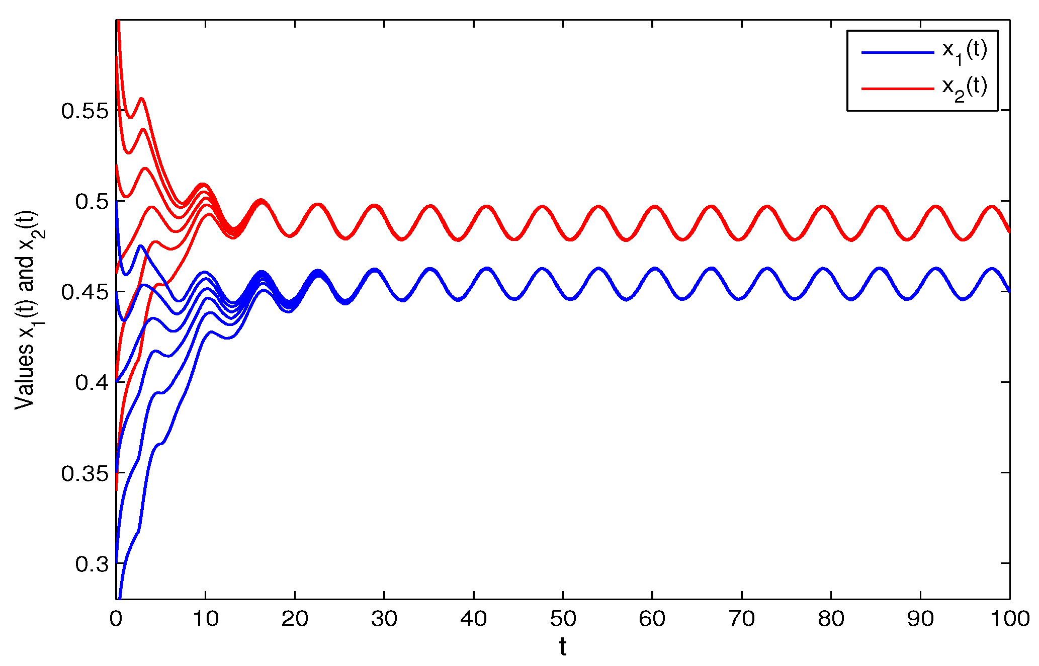
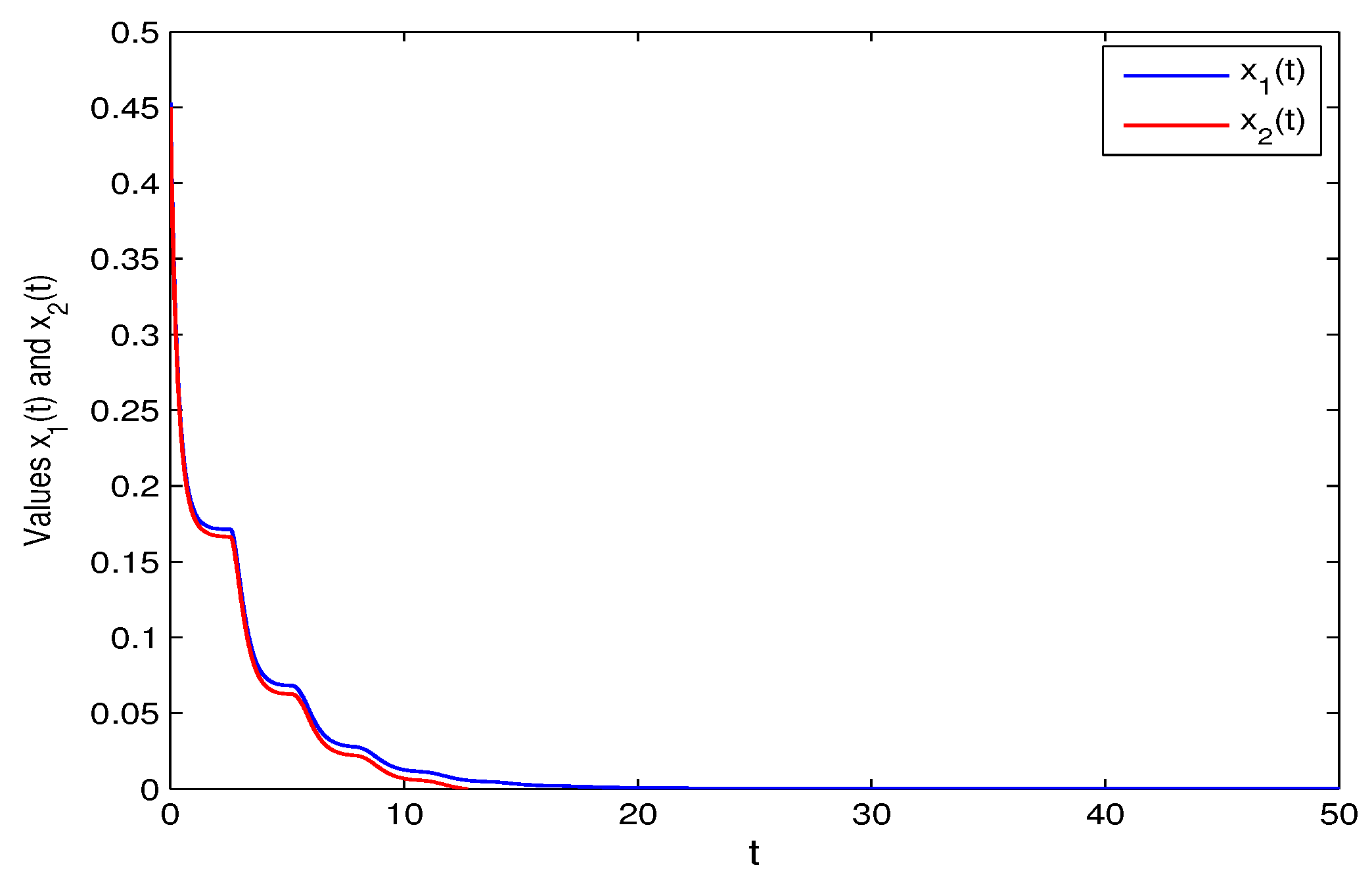
3. Numerical Examples

Here, we provide three examples to support the main results in this study.

Example 1.

$$\begin{array}{ll}\dot{x_1}\left(t\right)=& -(1.12+0.01cos\left(t\right))x_1\left(t\right)+(1.52+0.02cos\left(t\right))x_1(t-(0.5+0.1sin\left(t\right)))\\ & ·{\mathrm{e}}^{-(0.08+0.01cos\left(t\right))x_1(t-(0.5+0.1sin\left(t\right)))}-(0.075+0.01cos\left(t\right))x_1\left(t\right)x_2\left(t\right),\\ \dot{x_2}\left(t\right)=& -(1.12+0.01cos\left(t\right))x_2\left(t\right)+(1.52+0.02cos\left(t\right))x_2(t-(0.6+0.1sin\left(t\right)))\\ & ·{\mathrm{e}}^{-(0.08+0.01cos\left(t\right))x_2(t-(0.6+0.1sin\left(t\right)))}-(0.08+0.01cos\left(t\right))x_1\left(t\right)x_2\left(t\right).\end{array}$$

(41)

By calculating, we have

$$\min \{\underset{t\in R}{\inf }\frac{a\left(t\right)}{\delta \left(t\right)},\underset{t\in R}{\inf }\frac{\delta \left(t\right)}{k\left(t\right)}\}\approx 1.327,a^L\approx 1.5>\left({\delta }^M+\frac{a^M}{e{b}^L{\delta }^L}k\right)b^M{\mathrm{e}}^2\approx 1.1879.$$

Obviously, the coefficients of system (41) satisfy all the conditions of Corollary 1 and Theorem 1.

Remark 1.

From Figure 1, we find that the solution trajectories of system (41) stay bounded from above and below and do not diverge to infinity over time. This indicates that the permanence of system (41). In addition, the solution trajectories of system (41) repeat themselves in a cyclic manner. This means that the system reaches the same state after a certain period of time ($2\pi$—period of time), indicating the existence of $2\pi$—periodic solutions of system (41).

Example 2.

$$\begin{array}{ll}\dot{x_1}\left(t\right)=& -(1.35+0.01cos\left(t\right))x_1\left(t\right)+(2.52+0.02cos\left(t\right))x_1(t-(2.5+0.1sin\left(t\right)))\\ & \times {\mathrm{e}}^{-(1.01+0.01cos\left(t\right))x_1(t-(2.5+0.1sin\left(t\right)))}-(0.5+0.01cos\left(t\right))x_1\left(t\right)x_2\left(t\right),\\ \dot{x_2}\left(t\right)=& -(1.35+0.01cos\left(t\right))x_2\left(t\right)+(2.52+0.02cos\left(t\right))x_2(t-(2.6+0.2sin\left(t\right)))\\ & \times {\mathrm{e}}^{-(1.01+0.01cos\left(t\right))x_2(t-(2.6+0.2sin\left(t\right)))}-(0.42+0.1cos\left(t\right))x_1\left(t\right)x_2\left(t\right).\end{array}$$

(42)

By calculation, we derive that

$$\min \{\underset{t\in R}{\inf }\frac{a\left(t\right)}{\delta \left(t\right)},\underset{t\in R}{\inf }\frac{\delta \left(t\right)}{k\left(t\right)}\}\approx 1.838,D=\min \left\{D_1,D_2\right\}\approx \min \{0.177,0.129\}=0.129.$$

Then, the coefficients of system (42) satisfy all the conditions of Corollary 2.

Remark 2.

From Figure 2, we find the permanence and periodicity of system (42). Moreover, the solution trajectories of system (42) start from different initial conditions and finally converge towards a curve within a given interval. This indicates the global attractive periodic solution of system (42).

Example 3.

$$\begin{array}{ll}\dot{x_1}\left(t\right)=& -(3+0.02cos\left(t\right))x_1\left(t\right)+(1.22+0.02cos\left(t\right))x_1(t-(0.07+0.1sin\left(t\right)))\\ & \times {\mathrm{e}}^{-(0.14+0.01cos\left(t\right))x_1(t-(0.07+0.1sin\left(t\right)))}-(0.15+0.05cos\left(t\right))x_1\left(t\right)x_2\left(t\right),\\ \dot{x_2}\left(t\right)=& -(3+0.02cos\left(t\right))x_2\left(t\right)+(1.22+0.02cos\left(t\right))x_2(t-(0.08+0.1sin\left(t\right)))\\ & \times {\mathrm{e}}^{-(0.14+0.01cos\left(t\right))x_2(t-(0.08+0.1sin\left(t\right)))}-(0.17+0.045cos\left(t\right))x_1\left(t\right)x_2\left(t\right).\end{array}$$

(43)

By calculating, we can obtain ${\delta }^L\approx 2.98>a^M\approx 1.24$. Obviously, the coefficients of system (43) satisfy the condition of Lemma 5; then, system (43) is extinct.

Remark 3.

From Figure 3, we find that the solution trajectories of system (43) decrease over time and reach zero. This indicates the extinction of system (43).

4. Conclusions

It is well known that the motivation of the Nicholson’s blowflies model lies in its potential to expose the underlying principles that govern blowfly population dynamics and contribute to broader research fields such as pest control and ecological studies. Therefore, the study of Nicholson’s blowflies model is helpful to comprehend the dynamics of blowfly populations in order to address practical issues related to pest control, biology, and ecology. In this study, the dynamics of the competitive Nicholson’s blowflies model with time-varying coefficients and continuous time delays was investigated. By constructing appropriate Lyapunov functions and several useful inequalities, several criteria for the permanence, extinction, periodic solutions, and global attractiveness of the system were obtained. From this study, we found that the main results and system (6) can be seen as supplements and extensions of the previously results and systems [1,2,3,4,5,6,7,8,9,10,11,12].

On the other hand, stochastic population dynamical systems [9,10,15,17] refer to mathematical models that describe the changes in population size over time, taking into account the random fluctuations and uncertainties in environmental factors and demographic processes. These models are typically used in ecology, biology, and conservation biology to study the dynamics of populations and predict their future behaviors. Hence, we have interesting future work, for example, investigating the dynamic behavior on the stochastic Nicholson’s blowflies model with delays.

References

1. Gurney, W.S.C.; Blythe, S.P.; Nisbet, R.M. Nicholson’s blowflies revisited. Nature 1980, 287, 17–21. [Google Scholar] [CrossRef]
2. Saker, S.H.; Agarwal, S. Oscillation and global attractivity in a periodic Nicholson’s blowflies model. Math. Comput. Model. 2002, 35, 719–731. [Google Scholar] [CrossRef]
3. Berezansky, L.; Braverman, E.; Idels, L. Nicholson’s blowflies differential equations revisited: Main results and open problems. Appl. Math. Model. 2010, 34, 1405–1417. [Google Scholar] [CrossRef]
4. Berezansky, L.; Idels, L.; Troib, L. Global dynamics of Nicholson-type delay systems with applications. Nonlinear Anal. Real World Appl. 2011, 12, 436–445. [Google Scholar] [CrossRef]
5. Zhou, Q. The positive periodic solution for Nicholson-type delay system with linear harvesting terms. Appl. Math. Model. 2013, 37, 5581–5590. [Google Scholar] [CrossRef]
6. Jiang, J. Dynamic Properties of Competitive Nicholson’s Blowflies Model. Master’s Thesis, Hunan University, Changsha, China, 2011. [Google Scholar]
7. Muhammadhaji, A.; Halik, A. Dynamics in a nonautonomous Nicholson-type delay system. J. Math. 2021, 2021, 6696453. [Google Scholar] [CrossRef]
8. Ezekiel, I.D.; Iyase, S.A.; Anake, T.A. Stability analysis of a nontrivial solution for delayed Nicholson blowflies’ model with linear harvesting function. J. Phys. Conf. Ser. 2022, 2199, 012034. [Google Scholar] [CrossRef]
9. Wu, R.; Xu, Z. Spreading dynamics of a discrete Nicholson’s blowflies equation with distributed delay. Proc. R. Soc. Edinburgh Sect. A Math. 2023, 2023, 1–23. [Google Scholar] [CrossRef]
10. Mu, X.; Jiang, D.; Hayat, T.; Alsaedi, A.; Ahmad, B. Dynamical behavior of a stochastic Nicholson’s blowflies model with distributed delay and degenerate diffusion. Nonlinear Dyn. 2021, 103, 2081–2096. [Google Scholar] [CrossRef]
11. Long, X.; Gong, S. New results on stability of Nicholson’s blowflies equation with multiple pairs of time-varying delays. Appl. Math. Lett. 2020, 100, 106027. [Google Scholar] [CrossRef]
12. Li, D.; Wu, X.; Yan, S. Periodic traveling wave solutions of the Nicholson’s blowflies model with delay and advection. Electron. Res. Arch. 2023, 31, 2568–2579. [Google Scholar] [CrossRef]
13. Ding, X. Global asymptotic stability of a scalar delay Nicholson’s blowflies equation in periodic environment. Electron. J. Qual. Theory Differ. Equ. 2022, 2022, 14. [Google Scholar] [CrossRef]
14. Fan, W.; Zhang, J. Novel results on persistence and attractivity of delayed Nicholson’s blowflies system with patch structure. Taiwan. J. Math. 2023, 27, 141–167. [Google Scholar] [CrossRef]
15. Belmabrouk, N.; Damak, M.; Miraoui, M. Stochastic Nicholson’s blowflies model with delays. Int. J. Biomath. 2023, 16, 2250065. [Google Scholar] [CrossRef]
16. Muhammadhaji, A.; Halik, A. Dynamic analysis of a model for Spruce Budworm populations with delay. J. Funct. Spaces 2021, 2021, 1091716. [Google Scholar] [CrossRef]
17. Moujahid, A.; Vadillo, F. Impact of delay on stochastic predator-prey models. Symmetry 2023, 15, 1244. [Google Scholar] [CrossRef]
Figure 1. Permanence and periodicity of system (41).
Symmetry 15 01495 g001
Figure 2. Global attractive periodic solution of system (42).
Symmetry 15 01495 g002
Figure 3. Extinction of system (43).
Symmetry 15 01495 g003
Disclaimer/Publisher’s Note: The statements, opinions and data contained in all publications are solely those of the individual author(s) and contributor(s) and not of MDPI and/or the editor(s). MDPI and/or the editor(s) disclaim responsibility for any injury to people or property resulting from any ideas, methods, instructions or products referred to in the content.