Abstract
An infinite impulse response (IIR) system might comprise a multimodal error surface and accurately discovering the appropriate filter parameters for system modeling remains complicated. The swarm intelligence algorithms facilitate the IIR filter’s parameters by exploring parameter domains and exploiting acceptable filter sets. This paper presents an enhanced symmetric sand cat swarm optimization with multiple strategies (MSSCSO) to achieve adaptive IIR system identification. The principal objective is to recognize the most appropriate regulating coefficients and to minimize the mean square error (MSE) between an unidentified system’s input and the IIR filter’s output. The MSSCSO with symmetric cooperative swarms integrates the ranking-based mutation operator, elite opposition-based learning strategy, and simplex method to capture supplementary advantages, disrupt regional extreme solutions, and identify the finest potential solutions. The MSSCSO not only receives extensive exploration and exploitation to refrain from precocious convergence and foster computational efficiency; it also endures robustness and reliability to facilitate demographic variability and elevate estimation precision. The experimental results manifest that the practicality and feasibility of the MSSCSO are superior to those of other methods in terms of convergence speed, calculation precision, detection efficiency, regulating coefficients, and MSE fitness value.
1. Introduction
The IIR filter leverages the simplified scheme orders, fewer adjustable coefficients, and augmented spectrum allocation to accomplish high measurement precision and efficient convergence performance, which is frequently utilized in monitoring systems, wireless communication, signal manipulation, geographical exploratory, noise mitigation, and software-driven equalization. The error cost of the flexible IIR system identification is characterized by nonlinearity and non-differentiability. Numerous optimization techniques have recently been executed to construct the IIR filter system. The conventional design techniques utilize the Butterworth or Chebyshev Type I or Type II to design the IIR filter, which employs the bilinear transformation approach to convert the analog filter (s-domain) to the digital filter (z-domain). However, this technique has severe demerits in terms of the frequency-distorting effect, quantization errors, and nonlinear phase errors [1,2,3].
Later, gradient-based techniques such as Newton’s method, Quasi-Newton method, simplex technique, least mean square (LSM), linear programming, and least squares and its enhanced variants are used to resolve the IIR filter and minimize the error fitness value [4,5,6]. Most adaptive IIR filters are associated with nonlinear and multimodal fitness errors. These techniques are reliable and stable for the parameter estimation of a linear IIR system, and the unimodal objective function between an unidentified system’s input and the IIR filter’s output must be linear. However, these techniques have limitations: inefficient initial population quality, sluggish convergence acceleration, restricted evaluation precision, easy precocious convergence, slow detection efficiency, and combinatorial explosion. Meanwhile, these techniques exhibit some inherent demerits: the necessity of continuous and differentiable fitness, typically recognizing the regional extreme solution or retracing the sub-optimal solution, an inability to explore the enormous search domain, a constraint of the piecewise linear cost approximation (linear programming), and starting points becoming exceedingly sensitive as the solution variables increase [7,8]. They are uncertain and unstable when designing the higher-order systems of the IIR filter system because the poles may relocate the exterior of the unit circle.
Some swarm intelligence algorithms are applied to resolve the nonlinear, non-differentiable, multimodal, non-convex, and non-quadratic IIR system identification to overcome the above demerits. The swarm intelligence algorithms imitate the macro-intelligence characteristics and learning methods of groups of animals in nature, utilizing cooperation and information exchange to attain the most affordable and achievable solution. These algorithms exhibit parallel solid processing performance, global exploration ability, search efficiency, and strong adaptability to handle super-complex, large-scale, high-dimensional problems [9]. These algorithms establish single-objective and multi-objective mathematical models according to the different assessment environments and research objectives, which utilize different constraints and evaluation indicators to validate sustainability and feasibility and establish the most satisfactory value. These algorithms harmonize to the finest potential solution with faster detection efficiency and inhibit precocious convergence with superior escape ability. They ensure formidable discovery and extraction to recognize the most appropriate regulating coefficients and minimize the MSE.
The basic swarm intelligence algorithms are applied to resolve the IIR system identification and recognize the most appropriate regulating coefficients. Mahata et al. pursued a manta ray foraging approach to resolve the IIR system identification. The pole relating and initialization schedule ensured stability and reliability, which utilized chain, cyclone, and somersault scavenging to attain an attractive scavenging tactic and exemplary extraction efficiency to validate coherence and convergence. Still, it was impacted by an inappropriate selection of the fitness, robustness, resolution speed, and computational efficiency [10]. Izci et al. conducted a whale optimization approach to resolve IIR system identification, and this approach utilized circumnavigating prey, bubble-net assaulting, and pursuit for prey to stabilize localized exploitation and broad exploration to recognize the expansive accurate solution and the most appropriate regulation variables. The exploration and exploitation analysis of the proposed approach needed further research and discussion [11]. Singh et al. established a teaching-learning procedure to resolve the IIR system identification, and this approach utilized the average difference to maintain the diversity and robustness, advance extraction operation, and disrupted regional extreme solutions to identify the most satisfactory solution. The regulating coefficients, mean square error, convergence accuracy, and detection efficiency of the proposed approach needed to be further enhanced in addressing the higher-order IIR system identification [12]. Wang et al. explained an artificial fish swarm approach to resolve the IIR system identification, and this approach exhibited strong search ability and optimization efficiency to attain a lower ameliorated system error and greater estimated precision. However, the approach’s detection accuracy and convergence efficiency were associated with the appropriate selection of the control parameters, and the computational complexity was huge [13]. Ekinci et al. explored the atom search optimization to resolve IIR filter identification; this approach filtrated the finest potential solution, fostered selection probability, quickened the convergence procedure, and bolstered localized exploitation so that it maintained instructive sustainability and adaptability to prohibit search standstill and determine the finest global solution. The exploration and exploitation, diversity analysis, and hyperparameters tuning of the proposed algorithm needed further analysis and research [14].
However, the original algorithms may exhibit the demerits of slow convergence rate, low evaluation precision, and easy precocious convergence. To enhance convergence accuracy and detection efficiency, swarm intelligence algorithms with ensemble strategies are applied to resolve the identification of IIR systems. Zhang et al. devised a self-adaptation hybridized cross-mutation slime mold approach to resolve the IIR system identification; the Cauchy mutation operator augmented the mutation ability and evolutionary directions, the crossover rate equilibrium with differential vector information compensated for an individual-fitness relationship to expand the detection process, and the self-adaptation resume hybrid opposition learning elevated population diversity and alleviated search stagnation. This approach promoted and maintained instructive competitiveness and effectiveness to bolster resolution accuracy, a single objective approach with certain limitations in solving multi-objective issues [15]. Su et al. exploited the multi-objective particle swarm optimization to resolve the IIR system identification, and the approach incorporated the Pareto frontier efficiency and global detection ability to balance passband and stopband filter orders and qualitative concerns. The proposed approach significantly reduced the passband oscillation and maximized stopband suppression to ensure the predetermined indicators of the interrupted frequency and the IIR system order, which exhibited substantial sustainability and dependability in accomplishing the minimal fitness and facilitating regulation variables [16]. Rizk-Allah et al. developed sophisticated artificial rabbit optimization to solve the IIR filter identification. The adaptive local search mechanism reduced accuracy loss, enhanced local exploitation accuracy, and improved the optimization process, and the experience-based perturbed learning strategy promoted detection efficiency, increased population diversity, and avoided search stagnation. The sustainability and adaptability of the proposed approach are superior to those of other approaches in terms of the MSE fitness value, convergence accuracy, regulating coefficients, and evaluation efficiency [17]. Zhang et al. implemented an upgraded GJO to resolve the IIR filter identification, aiming to achieve the most appropriate regulating coefficients and minimize the mean square error. The elite opposition-based learning advanced demographic variety, promoted discovery efficiency, extended the detection domain, and avoided anticipation stagnation. The simplex approach accelerated the investigation of velocity, enhanced the extraction ability, fostered the estimation precision, and advanced the exploitation depth. The proposed approach advanced extraction operation and expedited evaluation efficiency to feature more enjoyable regulation variables and a more formidable convergence solution [18]. Niu et al. utilized an altered artificial ecosystem approach with a dynamical antagonistic learning tactic and the nonlinear adaptive weight coefficient to resolve IIR filter identification, and this approach facilitated population variety, fostered the extraction procedure, expedited evaluation efficiency, refrained precocious convergence, and bolstered broad exploration to maintain the finest potential solution [19].
The hybrid swarm intelligence algorithms are applied to bolster the exploration and exploitation and minimize the mean square error to resolve the IIR system identification. Kumar et al. incorporated a particle swarm optimization with a grasshopper optimization method to resolve IIR system identification; this approach exhibited remarkable intuitiveness and simplicity in identifying intelligent collaborative detection, accelerating exploitation efficiency, and facilitating solution accuracy, achieving a compensated estimation error. However, the proposed approach had limitations in the investigation research, parameter tuning process, computational complexity, and exploration and exploitation analysis [20]. Kaur et al. merged the chimp optimization approach with the cuckoo search approach to resolve IIR system identification; this approach combined exploration and exploitation to display sustainability and superiority in acquiring the most favorable evaluation solution and adjustment factors. However, the proposed approach’s convergence speed, estimation precision, and detection efficiency mainly depended on the appropriate selection of the regulating coefficients [21]. Ekinci et al. explored a cooperative technique with a gazelle optimization technique and simulated annealing method to resolve the IIR system identification; this approach not only achieved complementary advantages to avoid anticipation stagnation and enhance the detection efficiency, but also integrated prospecting and extracting to identify an extreme anticipation efficiency and identify precision.
Further research is needed to verify the stability and robustness of the control parameter adjustment and explore the adaptive technique of the proposed approach [22]. Ekinci et al. established a pattern search ameliorated arithmetic optimization technique to resolve the IIR system identification, and this approach utilized exploration and exploitation to fortify trustworthiness and dependability in accomplishing the superior regulation indicators and the highest-quality solution. The specific control parameters are associated with evaluation efficiency and estimation precision [23]. Liang et al. juxtaposed functional inequality-constrained optimization with a genetic algorithm to resolve IIR filter identification; this approach advanced initial population quality, escalated recognition depth, disrupted regional extreme solution, advanced extraction operation, and elevated estimation precision to improve convergence productivity and accomplished a more accurate solution [24].
Table 1 summarizes the brief literature review of existing methods for IIR system identification.

Table 1.
Brief literature review of existing methods for IIR system identification.
The SCSO is motivated by the distinguishable properties of sand cats and mimics the surveillance and neutralization of prey to recognize the low-frequency noise, the prey location, and the most appropriate solution [25]. The basic SCSO exhibits deficiencies, such as inefficient initial population quality, sluggish convergence acceleration, and restricted evaluation precision. Therefore, an enhanced symmetric SCSO with multiple strategies (MSSCSO) is presented to accomplish the benchmark functions and adaptive IIR filter identification. The no-free-lunch (NFL) theorem stipulates that no swarm intelligence algorithm can resolve each optimization-related difficulty, which motivates us to establish an enhanced symmetric SCSO. The main contributions are summarized: (1) The ranking-based mutation operator, elite opposition-based learning strategy, and simplex method are introduced into the basic SCSO to accelerate convergence efficiency and advance estimation accuracy. (2) The ranking-based mutation operator filtrates the finest potential solution, fosters selection probability, quickens the convergence procedure, and bolsters localized exploitation. (3) The elite opposition-based learning strategy facilitates demographic variability, upgrades searched an area, expedites evaluation efficiency, refrains precocious convergence, and bolsters broad exploration. (4) The simplex method advances initial population quality, escalates recognition depth, disrupts regional extreme solutions, advances extraction operation, and elevates estimation precision. (5) The MSSCSO is evaluated using the CEC 2022 and three sets of the IIR filter identification compared to recently published approaches. (6) The MSSCSO exhibits strong stability and robustness to balance exploration and exploitation to determine a swifter convergent velocity, greater explored accuracy, lower standard deviation, and more accurate fitness.
The subsequent sections constitute this article. Section 2 reviews SCSO. Section 3 extends MSSCSO. Section 4 summarizes the simulation test and result analysis for benchmark functions. Section 5 conveys MSSCSO-based adaptive IIR system identification. Section 6 discusses the exploration and exploitation analysis and the diversity analysis. Section 7 outlines the conclusion and future research.
2. SCSO
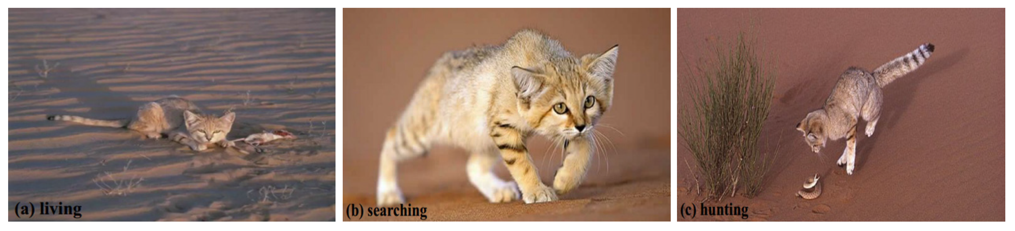
The SCSO is motivated by the sand cat’s extraordinary features, imitating the surveillance and neutralization of prey to recognize expansive, accurate solutions by detecting low-frequency noise and the prey’s location. Figure 1 articulates the sand cat’s distinguishable properties: living, searching, and hunting.
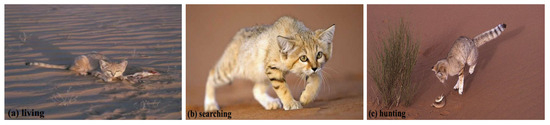
Figure 1.
Sand cat in nature: (a) living; (b) searching; (c) hunting.
2.1. Initial Population
The initialization matrix is constructed as follows:
where signifies the jth dimension of the ith sand cat.
The calculation matrix of fitness is constructed as follows:
2.2. Searching for Prey (Exploration)
The sand cat typically exploits low-frequency noise fabrication as an essential component of identifying and acquiring prey. The sensitivity will mitigate continuously from 2 to 0, which encourages the sand cat to gradually approach and capture prey without scaring it away or forfeiting it. The is constructed as follows:
where signifies the auditory traits, signifies the newest iteration, and signifies the highest iteration.
The and are constructed as follows:
The position vector is constructed as follows:
where signifies the optimal position, signifies the newest position.
2.3. Attacking on Prey (Exploitation)
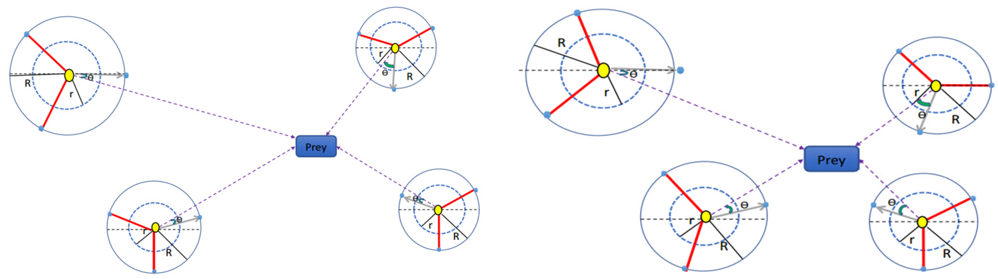
Each sand cat migrates in an alternative circumferential direction of the exploitation region if the sensitivity region is circle-shaped. Figure 2 articulates the position refreshing procedure of the SCSO. The SCSO deploys the Roulette Wheel Section to identify an arbitrary angle to investigate the harvesting position. This quickens the convergence procedure, expedites evaluation efficiency, refrains precocious convergence, and elevates estimation precision. The positions are constructed as follows:
where signifies the separation between the newest position and the ideal position , and signifies a random angle, .
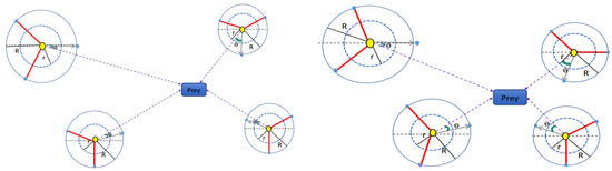
Figure 2.
Position refreshing procedure of SCSO: (a) iteration ; (b) iteration .
2.4. Exploration and Exploitation
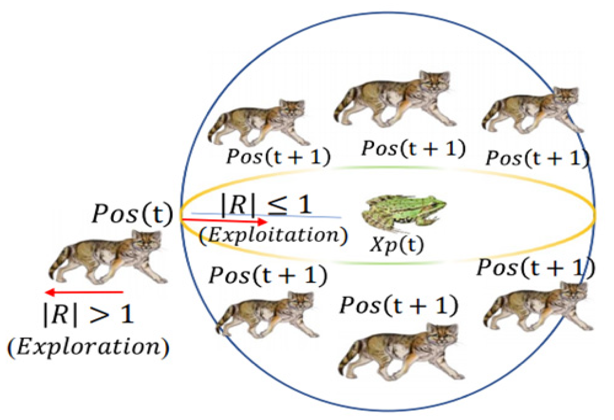
The SCSO seamlessly switches between localized exploitation and broad exploration to expedite evaluation efficiency and attain the finest potential solution. When , the SCSO instructs the sand cat to retrieve prey; it utilizes the Roulette Wheel Section to exploit and refrain from precocious convergence. When , the SCSO instructs the sand cat to determine a new potential solution, which operates a prey-seeking procedure to explore and pursue prey. Figure 3 articulates the attacking prey (exploitation) versus searching for prey (exploration). The positions are constructed as follows:

Figure 3.
Attacking prey (exploitation) versus searching for prey (exploration).
Algorithm 1 emphasizes the pseudocode of SCSO.
| Algorithm 1 SCSO |
| Begin Step 1. Randomly initialize the population, , and Step 2. Ascertain the sand cat’s fitness and identify the finest prey Step 3. while () do for each sand cat do Accomplish a randomized angle via Roulette Wheel Selection if () then Renew position via Equation (8) else Renew position via Equation (6) end if end for end while Restore the finest prey End |
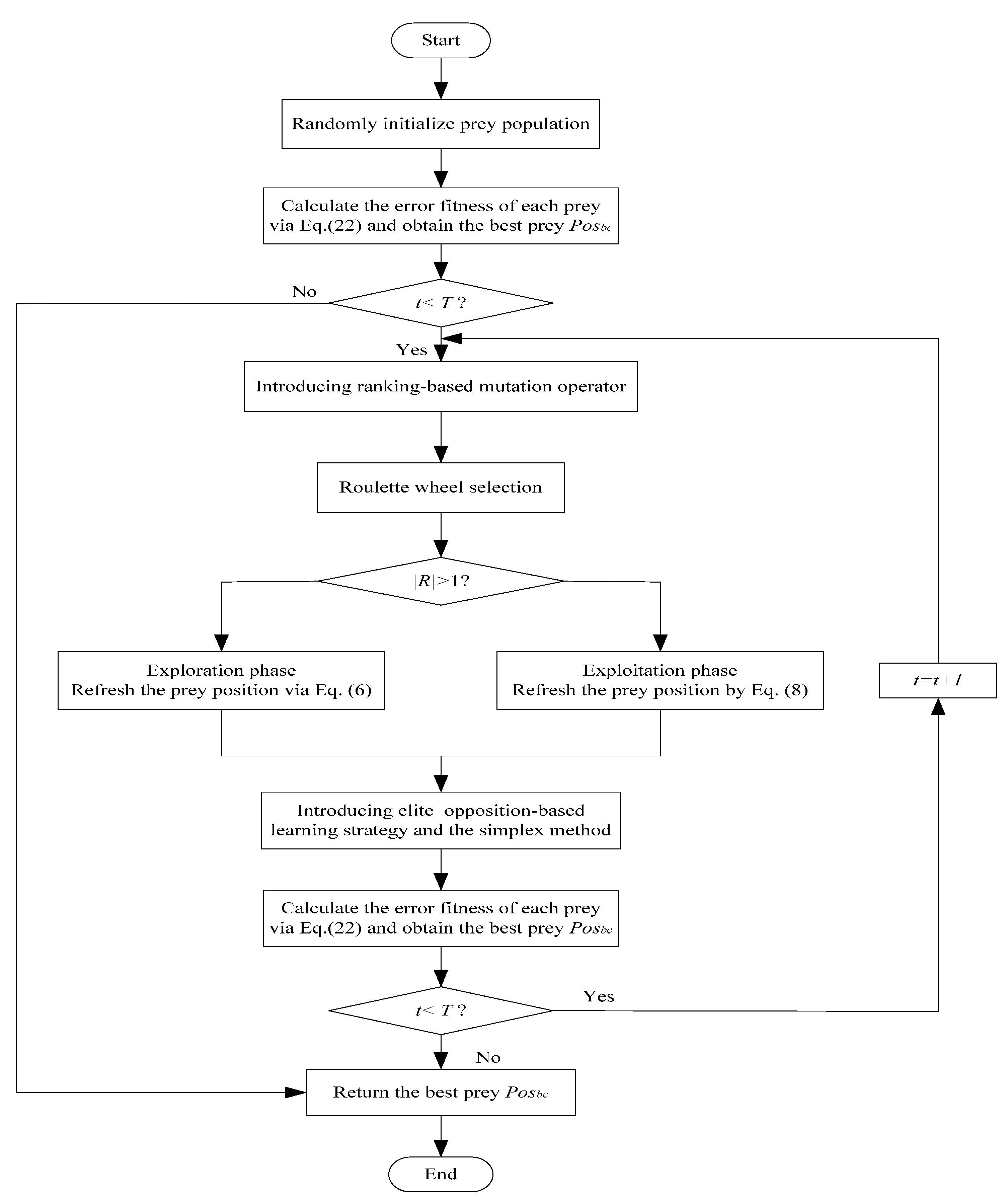
3. MSSCSO
To advance initial population quality, convergence acceleration, evaluation precision, and solution efficiency, the expanded MSSCSO maintains instructive sustainability and adaptability to realize supplementary advantages and refrain from precocious convergence, and this integrates localized exploitation and broad exploration to expedite evaluation efficiency and elevates estimation precision.
3.1. Ranking-Based Mutation Operator
This strategy filtrates the finest potential solution, fosters selection probability, quickens convergence procedure, and bolsters localized exploitation. The most desirable prey is assigned the finest search agent, and the fitness is sorted from most significant to poorest [26,27,28]. The ranking of sand cat is constructed as follows:
where signifies the population size. The selection probability is constructed as follows:
Algorithm 2 emphasizes the ranking-based mutation operator of “DE/rand/1”. Sand cats with the highest rating endure a more extensive probability of being established as the primordial vector or terminus vector, and the intention is to transmit the population’s genetic material to its descendants. A ranking-based mutation operator refrains from employing population sorting to ascertain the selection probability of the starting vector. The associated discovery procedure could dramatically diminish and facilitate voracious convergence if two differential variation vectors are extracted from the more prestigious vectors.
| Algorithm 2 Ranking-based mutation operator of “DE/rand/1” |
| Begin Sort the population and distribute the selection probability Automatically identify {base vector index} while Automatically identify end Automatically identify {terminal vector index} while Automatically identify end Automatically identify {starting vector index} while Automatically identify end End |
3.2. Elite Opposition-Based Learning Strategy
This strategy facilitates demographic variability, upgrades the search of an area, expedites evaluation efficiency, refrains from precocious convergence, and bolsters broad exploration. This approach specifies the most advantageous solution to serve as the search agent and executes the exploratory procedure by assessing the acceptable and the opposite solutions. A sand cat with the finest fitness is considered an elite solution [29,30,31]. The satisfactory solution and the opposite solution are constructed as follows:
where signifies the population size, signifies the dimension, , and and signify the dynamic boundaries, which together are constructed as follows:
The dynamic boundary may alter the inverse solution’s discovery region and preserve the most outstanding solution. The individual is constructed as follows:
3.3. Simplex Method
This strategy advances initial population quality, escalates recognition depth, disrupts regional extreme solutions, advances extraction operation, and elevates estimation precision, which identifies the optimality of a solution by replacing the original solution with a feasible solution [32,33,34]. Figure 4 articulates the simplex method schematically.
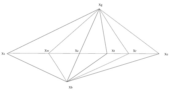
Figure 4.
Simplex method schematic.
- Step 1. Ascertain the fitness, filter out adequate solution , inadequate solution , and renewed solution , and ascertain the fitnesses , , and .
- Step 2. Ascertain the midpoint .
- Step 3. Ascertain the refraction point and the fitness .where signifies the reflectivity.
- Step 4. If , the extension operation is computed as follows:where signifies the extension factor. If , extension point replaces ; otherwise, replaces .
- Step 5. If , the compression operation is constructed as follows:where signifies the compression factor. If , compression point replaces ; otherwise, replaces .
- Step 6. If , the contraction point is computed as follows:where signifies the contraction factor. If , contraction point replaces ; otherwise, replaces .
Symmetry is an indispensable characteristic in methodologies and applications, and this is essential in multiple distinctive disciplines. Symmetry in algorithms frequently emphasizes patterns within data, streamlines complicated difficulties, and advances methodology efficiency. In this paper, we derive motivation from symmetric cooperative swarms. The entire sand cat swarm is separated into superior and inferior individuals, encouraging each individual to carry out the multiple responsibilities and occupations and facilitating the investigation and utilization of the solution region.
Algorithm 3 emphasizes the pseudocode of MSSCSO.
| Algorithm 3 MSSCSO |
| Begin Step 1. Randomly initialize the population, , and Step 2. Ascertain the sand cat’s fitness and identify the finest prey Step 3. while () do for each sand cat do Sort the population and distribute the selection probability /*ranking-based mutation stage*/ Automatically identify {base vector index} while Automatically identify end Automatically identify {terminal vector index} while Automatically identify end Automatically identify {starting vector index} while Automatically identify end /*end of ranking-based mutation stage*/ Accomplish a randomized angle via Roulette Wheel Selection if () then Renew position via Equation (8) else Renew position via Equation (6) end if The elite opposition-based learning strategy and simplex method are introduced into exploring and exploiting SCSO. end for end while Restore the finest prey End |
4. Simulation Test and Result Analysis for Benchmark Functions
4.1. Experimental Setup
The computerized instruments are executed on a Windows 10 PC with an Intel Core i7-8750H 2.2 GHz CPU, a GTX1060, and 8 GB RAM. All approaches are written and operated in MATLAB R2018b.
4.2. CEC 2022 Benchmark Functions
To assess the practicality and feasibility, the MSSCSO is used to resolve the function optimization. Table 2 summarizes the description of the CEC 2022 test suite [30,35].
Table 2.
Description of the CEC 2022 test suite.
4.3. Variables Setting
The MSSCSO is employed to resolve the CEC 2022, which is contrasted with bottlenose dolphin optimization (BDO) [36], Chornobyl disaster optimization (CDO) [37], golden jackal optimization (GJO) [38], Kepler optimization algorithm (KOA) [39], liver cancer algorithm (LCA) [40], spider wasp optimization (SWO) [41], rat swarm optimization (RSO) [42], hybrid leader-based optimization (HLBO) [43], waterwheel plant algorithm (WWPA) [44], sinh cosh optimization (SCHO) [45], and sand cat swarm optimization (SCSO) [25]. Each approach’s regulated variables are conventional speculative values extracted from the source papers.
BDO: accelerate factor , randomized factor , probability factor , positive constant .
CDO: gamma speed , beta speed , alpha speed , randomized value .
GJO: randomized value , randomized value , positive constant , randomized value , randomized value , positive constant .
KOA: positive constant , positive constant , positive constant .
LCA: randomized value , tumor , tumor , tumor , positive constant , radius .
SWO: tradeoff rate , crossover rate , randomized value , randomized value .
RSO: randomized value , randomized value .
HLBO: randomized value , integer value , positive constant .
WWPA: randomized value , randomized value , randomized value , exponential value , randomized value , randomized value .
SCHO: positive constant , randomized value , sensitive factor , sensitive factor , tiny positive value .
SCSO: sensitivity variable , phase control variable .
MSSCSO: sensitivity variable , phase control variable , randomized value , reflectivity , expansion coefficient , compression coefficient , contraction coefficient , scaling factor .
4.4. Sensitivity Analysis
This section discusses the sensitivity investigation of the hyperparameter tuning of MSSCSO by varying the scaling factor and keeping other parameters fixed.
Table 3 summarizes the sensitivity results of MSSCSO for the different scaling factors . For each approach, the average sample equals 50, the highest iteration equals 1000, and the detached operation equals 30. Best, Std, Mean, Median, and Worst signify the idealized value, standard deviation, average value, median value, and catastrophic value. To investigate the impact of the scaling factor on the convergence efficiency and estimation precision, the MSSCSO is carried out for several different values of the scaling factor taken as 0.1, 0.3, 0.5, 0.7, 0.9, 0.11, and 0.13, while keeping other parameters unchanged. The MSSCSO has a relatively good sensitivity to the scaling factor . The difference between the results of different scaling factors is significant. When the scaling factor is set to 0.7, MSSCSO receives excellent reliability and robustness to avoid anticipation stagnation and incorporates exploration and exploitation to achieve a swifter convergent velocity, greater explored accuracy, and more accurate fitness.
Table 3.
Sensitivity results of MSSCSO for the different scaling factors .
4.5. Simulation Test and Result Analysis
The MSSCSO is utilized to resolve the CEC 2022 test suite, which contains unimodal, essential, hybrid, and composite functions. The ranking is based on the catastrophic value.
Table 4 summarizes the simulation results of different approaches for the CEC 2022. To alleviate deficiencies of SCSO, such as inefficient initial population quality, sluggish convergence acceleration, and restricted evaluation precision, the ranking-based mutation operator, elite opposition-based learning strategy, and simplex method are incorporated into SCSO. For F1, F2, F3, F4, F5, and F10, the idealized values, standard deviations, average values, median values, and catastrophic values of the MSSCSO have been substantially augmented; the MSSCSO exhibits instructive sustainability and adaptability to refrain from precocious convergence and recognize the finest potential solution. The idealized values, standard deviations, average values, median values, and catastrophic values of MSSCSO are superior to those of BDO, CDO, GJO, KOA, LCA, SWO, RSO, HLBO, WWPA, SCHO, and SCSO. The MSSCSO utilizes the ranking-based mutation operator to filtrate the finest potential solution, foster selection probability, quicken the convergence procedure, and bolster localized exploitation. The MSSCSO utilizes broad discovery and localized extraction to enhance convergence acceleration and obtain better assessment metrics. The MSSCSO exhibits the most minor standard deviations and the best ranking, and it has strong stability and reliability. For F6 and F8, the standard deviations of the MSSCSO are worse than those of the SCSO. Still, the idealized values, standard deviations, average, median, and catastrophic values of the MSSCSO are more accurate than those of the BDO, KOA, LCA, SWO, RSO, HLBO, WWPA, and SCHO. The MSSCSO utilizes the elite opposition-based learning strategy to facilitate demographic variability, upgrade searched areas, expedite evaluation efficiency, refrain from precocious convergence, and bolster broad exploration. For F7, F9, F11, and F12, the MSSCSO has strong stability and reliability to enhance the idealized values, standard deviations, average, median, and catastrophic values. The assessment metrics and convergence efficiency of the MSSCSO have been substantially augmented. The idealized values, standard deviations, average, median, and catastrophic values of the MSSCSO are superior to those of the BDO, CDO, LCA, SWO, RSO, HLBO, SCHO, and SCSO. The MSSCSO utilizes the simplex method to advance initial population quality, escalate recognition depth, disrupt regional extreme solutions, advance extraction operation, and elevate estimation precision. The MSSCSO with symmetric cooperative swarms not only maintains instructive sustainability and adaptability to capture supplementary advantages and prohibit search standstill but also integrates prospecting and extracting to strengthen convergence productivity and accomplish the most satisfactory solution.
Table 4.
Simulation results of different approaches for the CEC 2022.
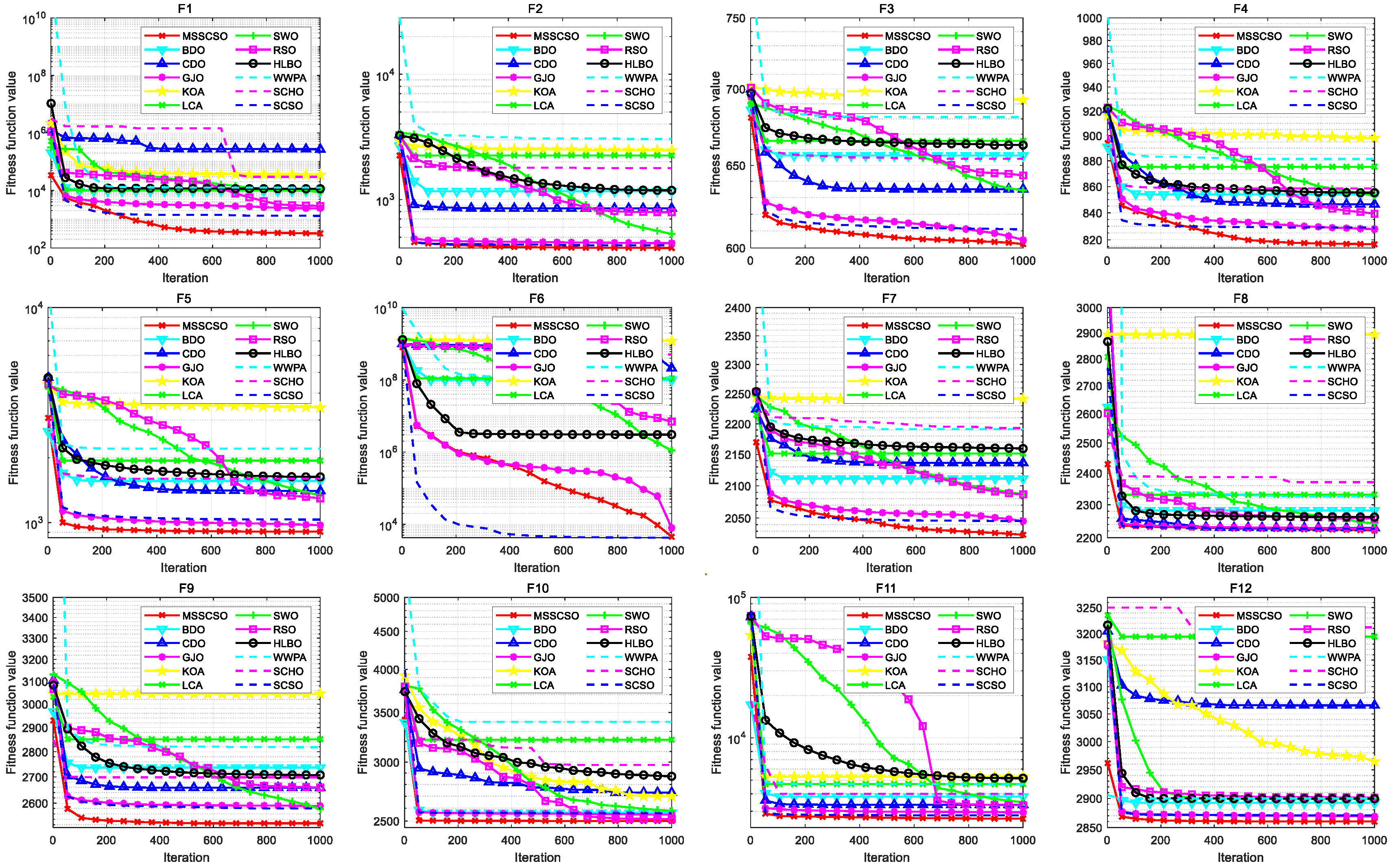
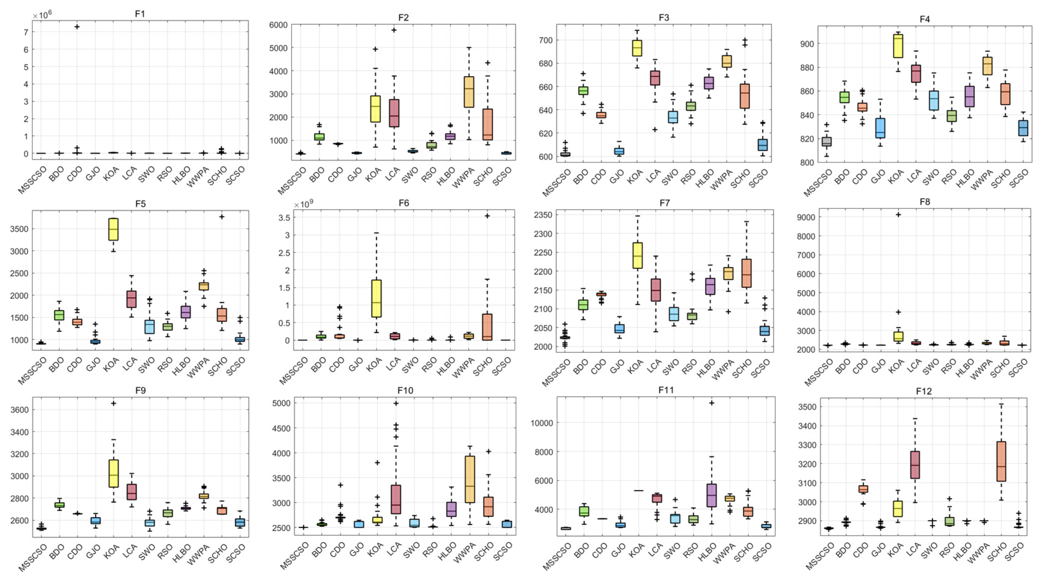
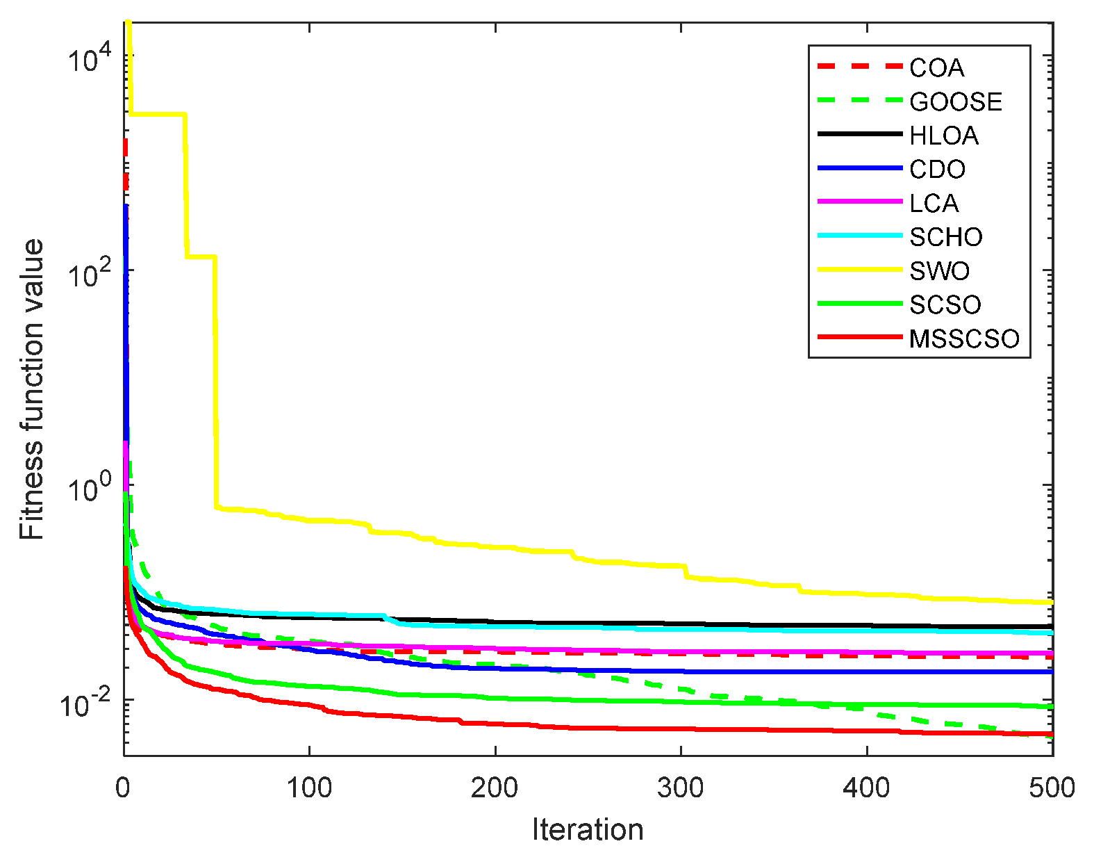
Figure 5 articulates the convergence trajectories of each approach. The convergence curve is a spontaneous technique used to visualize each approach’s utilization efficiency and resolution precision. When the comparison algorithms stabilize after a series of iterations, the approach exhibits superior evaluation precision and swifter utilization efficiency, which has instructive sustainability and adjustability to discover the most satisfactory solution. The MSSCSO endures an exceptional detection efficiency to mitigate anticipation stagnation and achieve the global optimal solution, which swiftly converges early and reliably re-explores later. The MSSCSO exhibits strong reliability and stability to incorporate discovery and extraction, superior convergence speed, calculation precision, and detection efficiency. For unimodal functions, essential functions, hybrid functions, and composite functions, the overall convergence efficiency and estimation precision of MSSCSO are superior to those of BDO, CDO, GJO, KOA, LCA, SWO, RSO, HLBO, WWPA, SCHO, and SCSO. The MSSCSO exhibits simple architectures, excessive optimization efficiency, marvelous parallelism, outstanding robustness, and stability, and it encounters excellent superiority and predictability in refraining from combinatorial explosion and precocious convergence. Figure 6 articulates the ANOVA tests of each approach. The standard deviation is a spontaneous technique to visualize each approach’s stability and reliability. The approach exhibits superior durability and dependability to foster optimization efficiency, advance extraction operation, and elevate estimation precision. The standard deviations of MSSCSO are superior to those of BDO, CDO, GJO, KOA, LCA, SWO, RSO, HLBO, WWPA, SCHO, and SCSO. The MSSCSO exhibits the formidable sustainability and dependability to disrupt the stagnation of exploration and recognize the most desirable solution. The MSSCSO incorporates the utilization and investigation to attain a swifter convergence velocity, greater estimation precision, superior regulation variables, lower standard deviation, and more accurate fitness.

Figure 5.
Convergence trajectories of each approach.
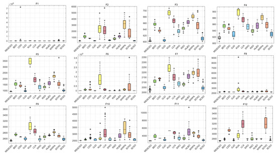
Figure 6.
ANOVA tests of each approach.
Table 5 summarizes the execution time of different approaches for the CEC 2022 test functions. For each approach, BDO is 189.2856 s, CDO is 51.8795 s, GJO is 67.0120 s, KOA is 76.1346 s, LCA is 48.2005 s, SWO is 43.2389 s, RSO is 38.7741 s, HLBO is 103.4885 s, WWPA is 65.2331 s, SCHO is 96.4285 s, SCSO is 52.2834 s, MSSCSO is 79.8849 s. The execution time of the MSSCSO is better than those of the BDO, HLBO, and SCHO, but worse than those of the CDO, GJO, KOA, LCA, SWO, RSO, WWPA, and SCSO. The ranking-based mutation operator, elite opposition-based learning strategy, and simplex method are introduced into the SCSO, which increases the execution time needed to identify the most satisfactory solution.
Table 5.
The execution time of different approaches for the CEC 2022 test functions.
Table 6 summarizes the results of the p-value Wilcoxon rank-sum test on the benchmark functions. Wilcoxon’s rank-sum test is administered to ascertain if MSSCSO differs noticeably from other approaches [46,47,48]. shows the distinguished discrepancy. shows no distinguished discrepancy. The experimental results demonstrate a distinguished discrepancy between MSSCSO and different approaches, and the data endure an appropriate degree of authenticity and dependability that was not established by accident.
Table 6.
Results of the p-value Wilcoxon rank-sum test on the benchmark functions.
5. MSSCSO-Based Adaptive IIR System Identification
5.1. Adaptive IIR System Identification
The MSSCSO is implemented to resolve the IIR system identification, and the principal objective is to recognize the most accurate regulating coefficients, minimize MSE between an unidentified system’s input and the IIR filter’s output, and match the unknown system’s transfer function. The adaptive IIR system exhibits some drawbacks: (1) It is unstable due to the inappropriate selection of denominator coefficients. The proper selection of search space overcomes this problem. (2) It cannot provide an exact linear phase response. The ranking-based mutation operator, elite opposition-based learning strategy, and simplex method are added to the SCSO to overcome drawbacks and improve the convergence speed and calculation accuracy. The MSSCSO maintains instructive stability and adaptability to capture supplementary advantages, prohibit discovery stagnation, and exhibit excellent global exploration and local exploitation to achieve the most satisfactory solution. The MSSCSO has strong robustness and reliability to minimize the MSE according to the stability of the IIR system, and the minimum solution of the MSE is regarded as the global optimal solution. System identification is advantageous for establishing a mathematical representation by investigating the unidentified structure’s input and the IIR filter’s output. Figure 7 articulates the adaptive IIR system identification via MSSCSO.
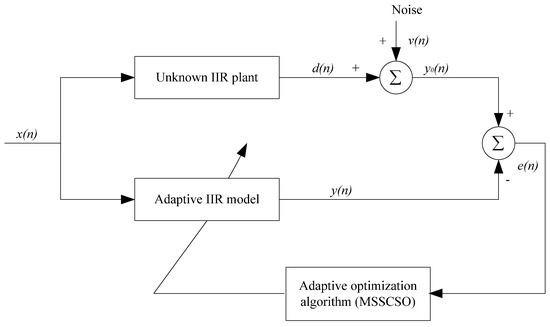
Figure 7.
The adaptive IIR system identification via MSSCSO.
The input and output of the IIR filter is constructed as follows:
where signifies the feedforward order, signifies the feedback, signifies the pole factor, and signifies the zero factor. The is constructed as follows:
The discrepancy between the unidentified system’s input and the IIR filter’s output is . The MSE is constructed as follows:
where signifies the input sample size and signifies the coefficient factor, .
The simple steps of the proposed model are summarized as follows:
- (1)
- Give the input variable and output variable of the adaptive IIR system identification.
- (2)
- Establish the mathematical expression for the IIR filter’s input and output; the formula is .
- (3)
- Introduce noise disturbance and an adaptive optimization algorithm (MSSCSO).
- (4)
- Utilize the unknown IIR system and adaptive IIR systems to construct the transfer function of the IIR filter .
- (5)
- Establish the fitness evaluation function of the mean square error (MSE) between an unidentified system’s input and the IIR filter’s output. The MSE is .
5.2. MSSCSO-Based Adaptive IIR System Identification
Algorithm 4 emphasizes the MSSCSO-based adaptive IIR system identification. Figure 8 articulates the flowchart of MSSCSO for adaptive IIR system identification.
| Algorithm 4 MSSCSO-based adaptive IIR system identification |
| Begin Step 1. Randomly initialize the population,, and Step 2. Ascertain the error fitness via Equation (22) and identify the finest prey Step 3. while () do for each sand cat do Sort the population and distribute the selection probability /*ranking-based mutation stage*/ Automatically identify {base vector index} while Automatically identify end Automatically identify {terminal vector index} while Automatically identify end Automatically identify {starting vector index} while Automatically identify end /*end of ranking-based mutation stage*/ Accomplish a randomized angle via Roulette Wheel Selection if () then Renew position via Equation (8) else Renew position via Equation (6) end if The elite opposition-based learning strategy and simplex method are introduced into the exploration and exploitation of SCSO. Ascertain the error fitness via Equation (22) end for end while Restore the finest prey End |
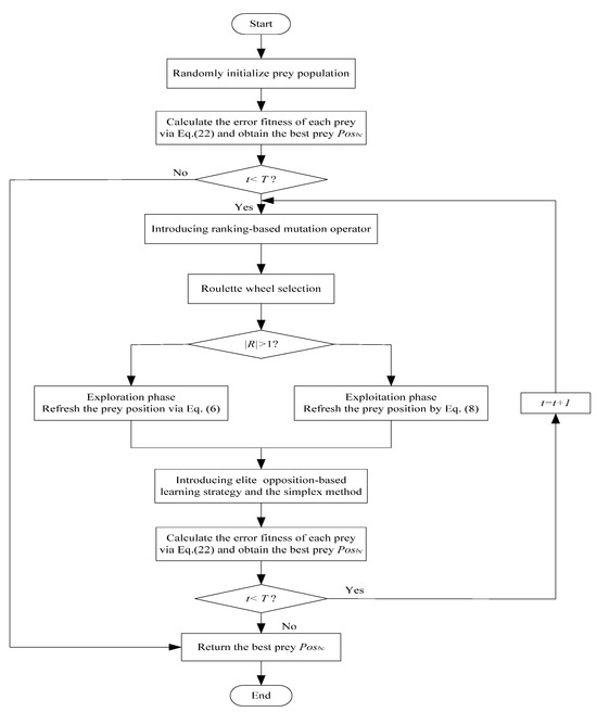
Figure 8.
Flowchart of MSSCSO for adaptive IIR system identification.
5.3. Computational Complexity of MSSCSO
Time complexity: This measures each algorithm’s computational time and resource consumption to resolve the optimization issues. The big-O notation efficiently verifies the stability and reliability. The time complexity mainly relies on the population size, the maximum iteration, and the issue dimension. The ranking-based mutation operator, elite opposition-based learning strategy, and simplex method are added to the SCSO to promote exploration and exploitation. The MSSCSO contains three main parts: population initialization, searching for prey (exploration) and attacking prey (exploitation), updating the sand cat’s location, and halting judgment. In MSSCSO, the population size is , the maximum iteration is , and the issue dimension is . The population initialization is . The searching for prey (exploration) is . The attacking on prey (exploitation) is . The updating of the sand cat’s location is . The updating of the sand cat’s location with the ranking-based mutation operator, elite opposition-based learning strategy, and simplex method is . The halting judgment is . Therefore, the total time complexity of MSSCSO is . Removing lower-order terms, the overall time complexity of the MSSCSO is .
Space complexity: This is measured by an algorithm’s additional storage. In MSSCSO, the population size is and the issue dimension is . The MSSCSO with symmetric cooperative swarms maintains instructive sustainability and adaptability to capture supplementary advantages, prohibit search standstill, and identify the most satisfactory solution. The overall space complexity of the MSSCSO is . The space efficiency of the MSSCSO is effective and stable.
5.4. Variables Setting
The MSSCSO is implemented to accomplish the IIR filter, which is contrasted with the coati optimization algorithm (COA) [49], GOOSE (GOOSE) [50], horned lizard defense tactics (HLOA) [51], Chornobyl disaster optimization (CDO) [37], liver cancer algorithm (LCA) [40], sinh cosh optimization (SCHO) [45], spider wasp optimization (SWO) [41], and sand cat swarm optimization (SCSO) [25]. Each approach’s regulated variables are conventional speculative values extracted from the source papers.
COA: randomized value , integer value .
GOOSE: weight of stone , randomized value , randomized value , randomized value .
HLOA: hue angle , positive constant , randomized value , randomized value , randomized value , randomized value .
CDO: gamma speed , beta speed , alpha speed , randomized value .
LCA: randomized value , tumor , tumor , tumor , positive constant , radius .
SCHO: positive constant , randomized value , sensitive factor , sensitive factor , tiny positive value .
SWO: tradeoff rate , crossover rate , randomized value , randomized value .
SCSO: sensitivity variable , phase control variable .
MSSCSO: sensitivity variable , phase control variable , randomized value , reflectivity , expansion coefficient , compression coefficient , contraction coefficient , scaling factor .
5.5. Simulation Test and Result Analysis
The MSSCSO maintains instructive sustainability and adaptability to capture supplementary advantages and prohibit search standstill, which integrates investigation and extraction to strengthen utilization efficiency and accomplish the most satisfactory solution.
For case 1, each approach facilitates a first-order IIR filter to recognize a second-order procedure; the unidentified procedure and IIR filter are constructed as follows:
For case 2, each approach facilitates a second-order IIR filter to recognize a second-order procedure; the unidentified system and IIR filter are constructed as follows:
For case 3, each approach facilitates a higher-order IIR filter to recognize a higher-order procedure; the unidentified system and IIR filter are constructed as follows:
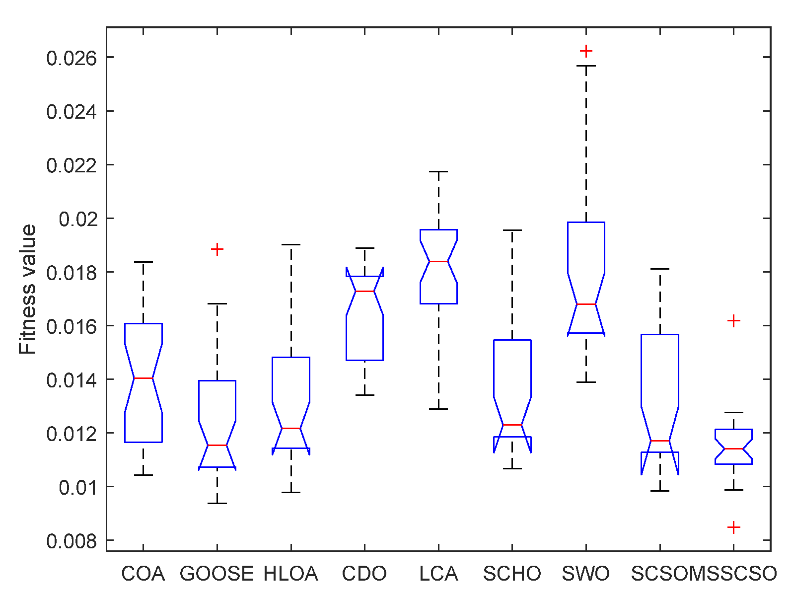
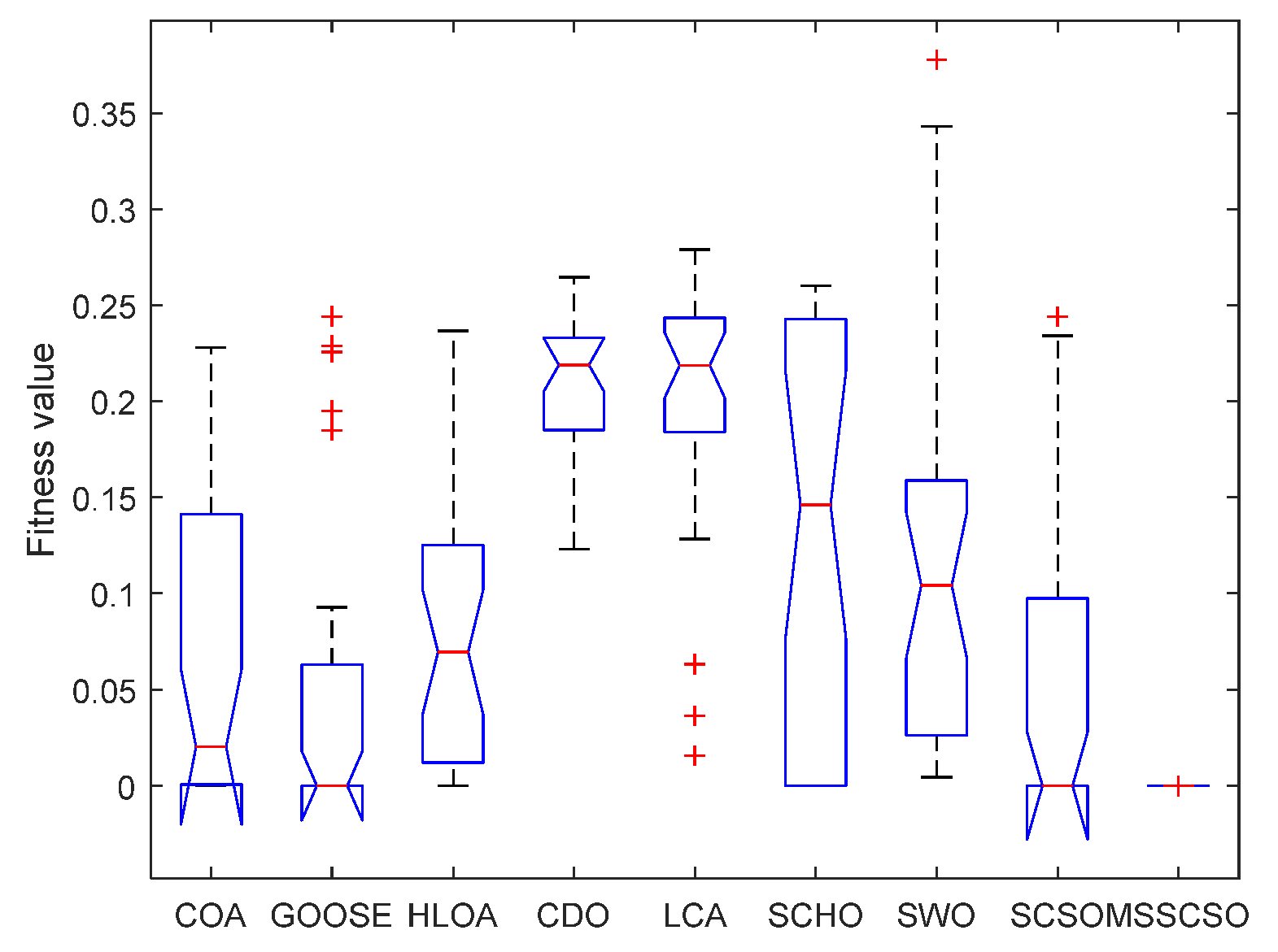
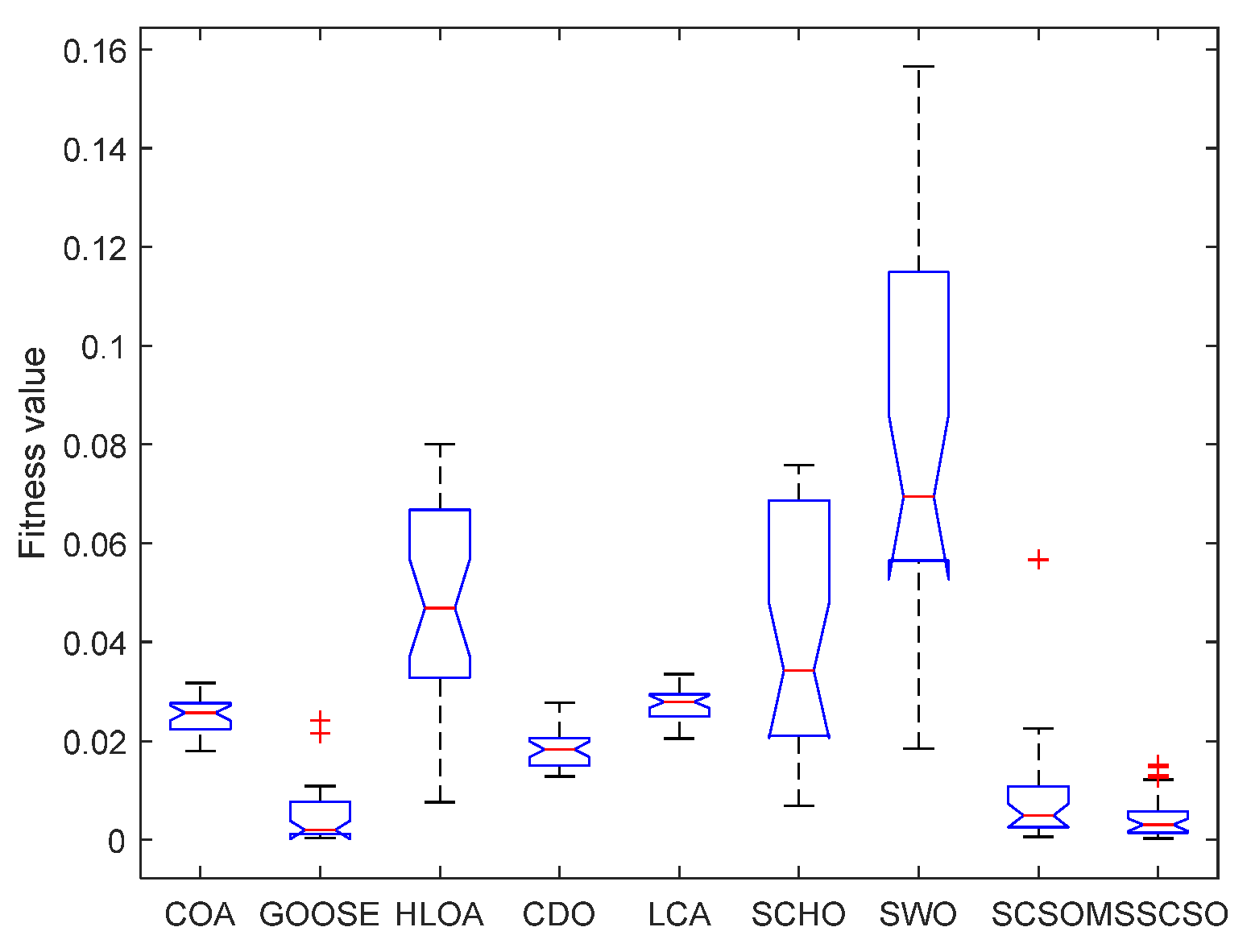
The MSSCSO is executed to eliminate the adaptive IIR system identification, and the principal objective is to establish the most appropriate regulation variables and the minimum achievable solution, which diminishes the estimation error between an unidentified system’s input and the IIR filter’s output. Table 7 summarizes each approach’s experimental results (MSE) for case 1. Table 8 summarizes the finest evaluation variables of each approach for case 1. Table 9 summarizes the average evaluation variables of each approach for case 1. Table 10 summarizes each approach’s experimental results (MSE) for case 2. Table 11 summarizes the finest evaluation variables of each approach for case 2. Table 12 summarizes the average evaluation variables of each approach for case 2. Table 13 summarizes each approach’s experimental results (MSE) for case 3. Table 14 summarizes the finest evaluation variables of each approach for case 3. Table 15 summarizes the average evaluation variables of each approach for case 3. For each approach, the average sample equals 30, the highest iteration equals 500, and the detached operation equals 30. Best, Worst, Mean, and Std signify the idealized value, catastrophic value, average value, and standard deviation, which comprehensively confirm the sustainability and profitability of MSSCSO. The ranking is established by measuring the standard deviation. To alleviate the deficiencies of the inefficient initial population quality, sluggish convergence acceleration, and restricted evaluation precision, the expanded MSSCSO is implemented to accomplish the IIR filter. For case 1, the assessment metrics of the MSSCSO are more accurate than those of the COA, GOOSE, HLOA, CDO, LCA, SCHO, SWO, and SCSO, and the MSSCSO encounters courageous investigation and extraction to refrain from sluggish searching and accomplish the most satisfactory solution. The finest or average evaluation variables of the MSSCSO are superior to those of the COA, GOOSE, HLOA, CDO, LCA, SCHO, SWO, and SCSO, and the MSSCSO receives fantastic consistency and endurance to ascertain the most effective evaluation variables. For case 2, the evaluation precision and solution efficiency of the MSSCSO have been substantially advanced compared to the SCSO. The assessment metrics and the finest or average evaluation variables of the MSSCSO are superior to those of the COA, GOOSE, HLOA, CDO, LCA, SCHO, SWO, and SCSO. The MSSCSO maintains discovery and extraction to attain a swifter convergence velocity, greater estimation precision, superior evaluation variables, lower standard deviation, and more accurate fitness. For case 3, the Best, Worst, and Mean of the MSSCSO are more precise than those of the COA, GOOSE, HLOA, CDO, LCA, SCHO, SWO, and SCSO, and the MSSCSO maintains instructive sustainability and adaptability to capture supplementary advantages and prohibit search standstill. The Std and ranking of the MSSCSO are superior to those of the GOOSE, HLOA, SCHO, SWO, and SCSO, but worse than those of the COA, LCA, and CDO, and the MSSCSO exhibits relative stability and robustness. The experimental results indicate that MSSCSO integrates prospecting and extracting to strengthen convergence productivity and accomplish the most satisfactory solution.
Table 7.
Experimental results (MSE) of each approach for case 1.
Table 8.
The finest evaluation variables of each approach for case 1.
Table 9.
The average evaluation variables of each approach for case 1.
Table 10.
Experimental results (MSE) of each approach for case 2.
Table 11.
The finest evaluation variables of each approach for case 2.
Table 12.
The average evaluation variables of each approach for case 2.
Table 13.
Experimental results (MSE) of each approach for case 3.
Table 14.
The finest evaluation variables of each approach for case 3.
Table 15.
The average evaluation variables of each approach for case 3.
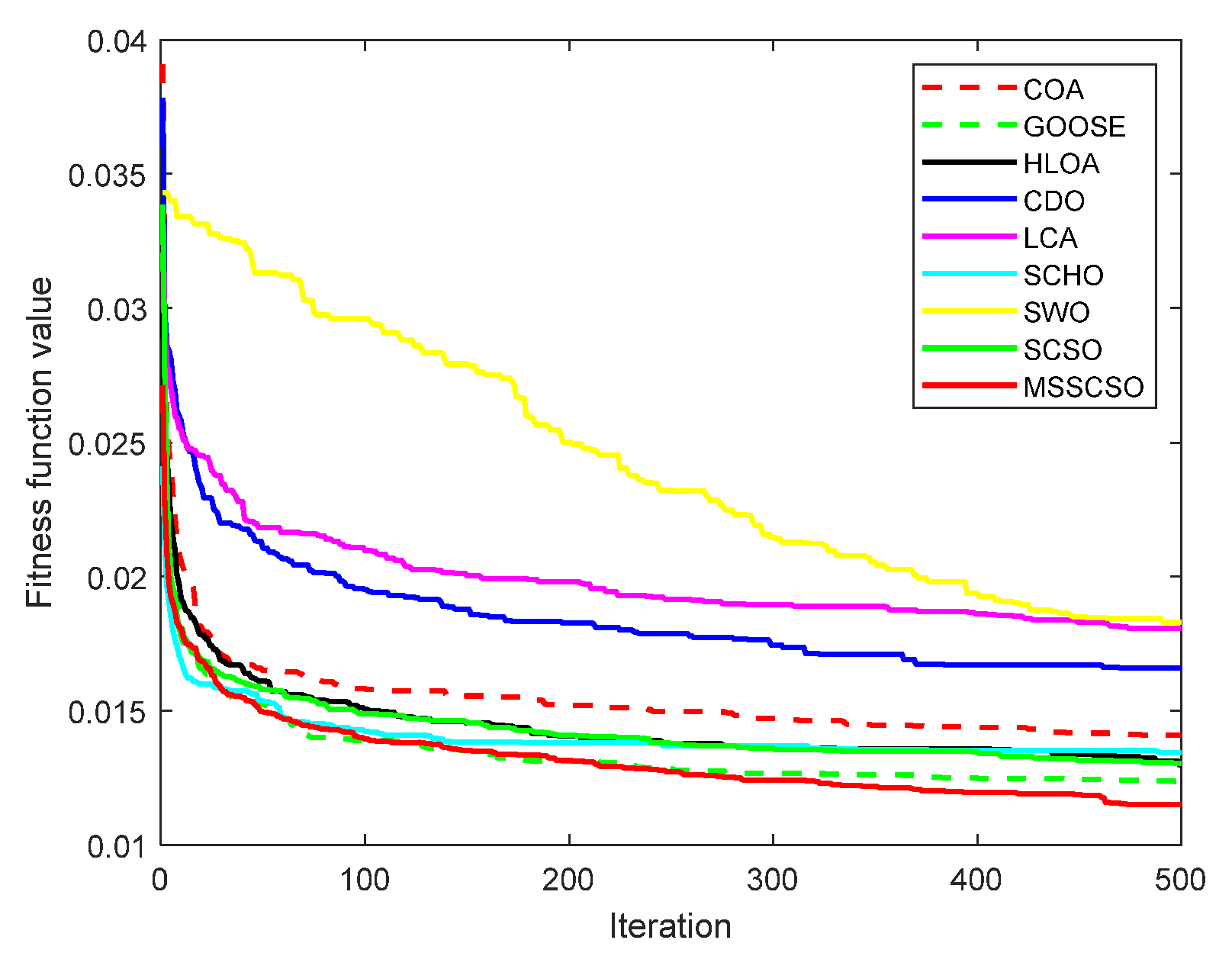
Figure 9 articulates the convergence trajectories of each approach for case 1. Figure 10 articulates the ANOVA tests of each approach for case 1. Figure 11 articulates the convergence trajectories of each approach for case 2. Figure 12 articulates the ANOVA tests of each approach for case 2. Figure 13 articulates the convergence trajectories of each approach for case 3. Figure 14 articulates the ANOVA tests of each approach for case 3. The MSSCSO is impacted by the scaling factor and the distinguishable properties of sand cats, which makes MSSCSO converge toward the optimal solution faster than other comparison approaches and subsequently re-exploit the evaluation accuracy. The overall convergence velocity and estimation precision of the MSSCSO for cases 1, 2, and 3 are superior to those of the COA, GOOSE, HLOA, CDO, LCA, SCHO, SWO, and SCSO; the MSSCSO not only maintains an equilibrium between localized extraction and nationwide investigation to restrict explore stagnation and strengthen convergence acceleration but also fosters selection probability and facilitates population variety to elevate estimation precision and expedite evaluation efficiency. For cases 1 and 2, the standard deviations of the MSSCSO are superior to those of the COA, GOOSE, HLOA, CDO, LCA, SCHO, SWO, and SCSO. The MSSCSO portrays noteworthy sustainability and superiority in recognizing the best solution and evaluation variables. For case 3, the standard deviation of the MSSCSO is superior to those of the GOOSE, HLOA, SCHO, SWO, and SCSO, but is worse than those of the COA, LCA, and CDO. The MSSCSO encounters relative stability and reliability to disrupt regional extreme solutions, foster convergence acceleration, bolster evaluation precision, and advance solution efficiency. The MSSCSO exhibits instructive sustainability and adaptability to foster selection probability, quicken the convergence procedure, bolster localized exploitation and broad exploration, facilitate population variety, broaden the searched area, refrain from precocious convergence, advance initial population quality, escalate recognition depth, and advance extraction operation. The experimental results manifest that MSSCSO maintains discovery and extraction to attain a swifter convergence velocity, greater estimation precision, superior regulation variables, lower standard deviation, and more accurate fitness.
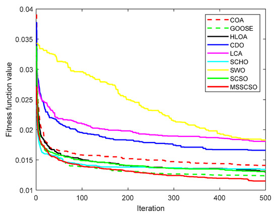
Figure 9.
Convergence trajectories of case 1.
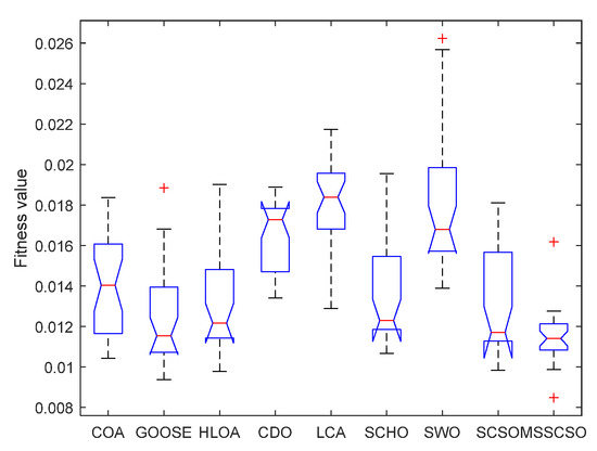
Figure 10.
ANOVA tests of case 1.
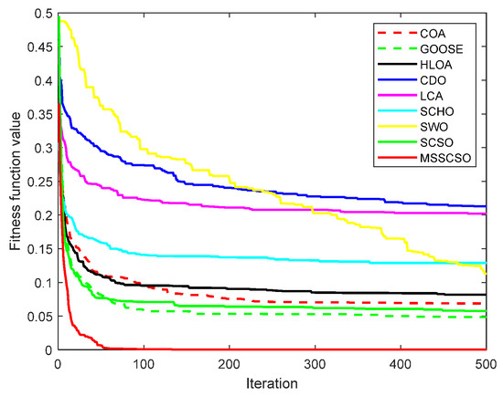
Figure 11.
Convergence trajectories of case 2.

Figure 12.
ANOVA tests of case 2.

Figure 13.
Convergence trajectories of case 3.

Figure 14.
ANOVA tests of case 3.
Table 16 summarizes the execution time of different approaches for cases 1, 2, and 3. For MSSCSO, the execution time of case 1 is 8.9495 s, the execution time of case 2 is 9.8702 s, and the execution time of case 3 is 10.6880 s. The overall execution time of the MSSCSO is better than that of the COA, GOOSE, HLOA, and CDO, but it is worse than that of the LCA, SCHO, SWO, and SCSO. The MSSCSO exhibits strong stability and robustness to balance exploration and exploitation and achieve a more accurate solution.
Table 16.
The execution time of different approaches for cases 1, 2, and 3.
Table 17 summarizes the results of the p-value Wilcoxon rank-sum test. The experimental results demonstrate a distinguished discrepancy between MSSCSO and other approaches, and the data endure an appropriate degree of authenticity and dependability that was not established by accident.
Table 17.
Results of the p-value Wilcoxon rank-sum test.
6. Exploration and Exploitation Analysis, Diversity Analysis
Exploration and exploitation are two essential search properties that inhibit precocious convergence, facilitate detection quality, and achieve the most satisfactory solution. There is a robust relationship between the exploration and exploitation of the unique search mechanism and the convergence accuracy. MSSCSO employs exploration to create low-frequency noise fabrication, search for prey, and capture prey, which is conducive to establishing the most appropriate solution in the search region and reducing the convergence efficiency of the optimization approach. The MSSCSO not only utilizes the exploitation to assault and retrieve prey but also utilizes the Roulette Wheel Section to refrain from precocious convergence, which is conducive to accelerating the convergence speed and advancing the possibility of regional extreme solutions. The appropriate ratio between exploration and exploitation is necessary to ensure the MSSCSO’s reasonable performance. The MSSCSO has strong overall searchability, stability, and robustness.
The MSSCSO is employed to accomplish the CEC 2022 and the adaptive IIR system identification, which utilizes a set of better candidate solutions to achieve exploration and exploitation, recognize the most satisfactory solution, and minimize the estimation error between an unidentified system’s input and the IIR filter’s output. Generally, the sand cat with the superior solution can guide the entire search process to achieve global exploration and local exploitation. When the distance between the sand cats gradually increases, the exploration’s impact will become progressively more apparent, and the exploitation’s impact will gradually weaken. A diversity measurement evaluates the increase and decrease in distance between the sand cats. The population diversity is constructed as follows:
where signifies the median of the jth dimension, signifies the jth dimension of ith sand cat, signifies the population size, and signifies the design variables. The mathematical expression to measure the percentage of exploration and exploitation is constructed as follows:
where signifies the maximum diversity. The two elements of exploration and exploitation are both mutually conflicting and complementary. In evaluating the balance impact, the median value utilizes the reference element to avoid optimization discrepancies, and the balance impact is affected by in the entire optimization process. The is employed as a reference to evaluate the rate of exploration and exploitation. The experimental results indicate that MSSCSO integrates exploration and exploitation to exhibit a swifter convergent velocity, greater explored accuracy, superior regulation variables, lower standard deviation, and more accurate fitness.
7. Conclusions and Future Research
The SCSO is motivated by the distinguishable properties of sand cats and mimics the surveillance and neutralization of prey to recognize the low-frequency noise, the prey location, and the most appropriate solution. The ranking-based mutation operator, elite opposition-based learning strategy, and simplex method are incorporated into the SCSO to enrich the population quality, convergence acceleration, evaluation precision, and solution efficiency. The expanded MSSCSO with symmetric cooperative swarms is implemented to accomplish the benchmark functions and adaptive IIR filter identification, and the principal objective is to recognize the most appropriate regulating variables and minimize the estimation error between an unidentified system’s input and the IIR filter’s output. The ranking-based mutation operator filtrates the finest potential solution, fosters selection probability, quickens the convergence procedure, and bolsters localized exploitation. The elite opposition-based learning strategy facilitates demographic variability, upgrades the search of an area, expedites evaluation efficiency, refrains from precocious convergence, and bolsters broad exploration. The simplex method advances initial population quality, escalates recognition depth, disrupts regional extreme solution, advances extraction operation, and elevates estimation precision. The MSSCSO exhibits simple architectures, excessive optimization efficiency, marvelous parallelism, outstanding robustness, and stability. The MSSCSO encounters excellent superiority and predictability in refraining from combinatorial explosion and precocious convergence. The experimental results demonstrate that MSSCSO incorporates the utilization and investigation to attain a swifter convergent velocity, greater explored accuracy, superior regulation variables, lower standard deviation, and more accurate fitness.
The limitations of the MSSCSO are summarized as follows: (1) The simulation experiments are primarily focused on the adaptive IIR system identification, and further investigations are needed to explore the optimization efficiency and convergence accuracy in a broader range of application fields. (2) The hyperparameters tuning process may require careful consideration to achieve the most satisfactory solution for different problem domains. (3) The proposed algorithm consumes more execution time to recognize the most appropriate regulating coefficients and minimize the MSE. (4) The computational complexity, mathematical logic reasoning, algorithm convergence proof, and dynamic parameter selection will affect the convergence speed and calculation accuracy. (5) The convergence efficiency and estimation accuracy of MSSCSO need to be further strengthened by introducing advanced search strategies, alternative encoding formats, and hybrid algorithmic structures to capture supplementary advantages and inhibit precocious convergence. (6) The MSSCSO is utilized to resolve super-complex, large-scale, high-dimensional, and multi-objective optimization problems, which may not be able to effectively balance exploration and exploitation to determine the finest potential solution.
Our future research will focus on the following aspects: (1) We will utilize more different IIR filter examples or large-scale engineering problems to evaluate and validate the effectiveness and stability of the MSSCSO. The MSSCSO will be compared with state-of-the-art methods to show its competitive performance. We will use statistical analysis to illustrate the discrepancies between the two data sets. (2) We will verify the algorithm convergence and computational complexity from theoretical and practical perspectives. We will exploit dynamic control parameters to enhance the stability and robustness. (3) We will execute advanced search strategies, alternative encoding formats, and hybrid algorithmic structures to capture supplementary advantages and avoid precocious convergence. The renewed SCSO will integrate localized exploitation and broad exploration to strengthen population quality, convergence acceleration, evaluation precision, and solution efficiency. (4) The renewed SCSO will be executed to improve characteristic Dabie Mountain forestry and crops, incorporating Huoshan Dendrobium, Lu’an Guapian, Chinese herbal medicine, and Shucheng Camellia oleifera. The quality of agricultural equipment and intelligent operation will be strengthened by intelligent detection, intelligent control, and specialized agricultural equipment.
Author Contributions
Conceptualization, J.Z. and C.D.; methodology, J.F.; software, C.D.; validation, J.Z., C.D. and J.F.; formal analysis, J.F.; investigation, C.D.; resources, J.Z.; data curation, C.D.; writing—original draft preparation, C.D.; writing—review and editing, J.Z. and J.F.; visualization, J.F.; supervision, C.D.; project administration, J.Z.; funding acquisition, J.Z., C.D. and J.F. All authors have read and agreed to the published version of the manuscript.
Funding
This research was funded by Start-up Fee for Scientific Research of High-level Talents of West Anhui University under Grant No. WGKQ2022052, School-level Quality Engineering (School-enterprise Cooperation Development Curriculum Resource Construction) under Grant No. wxxy2022101, School-level Quality Engineering (Teaching and Research Project) under Grant No. wxxy2023079, PWMDIC design and application under Grant No. WXCHX0045023110, and Natural Science Key Research Project of Anhui Educational Committee under Grant No. 2022AH051675.
Data Availability Statement
All data used to support the findings of this study are included within the article.
Acknowledgments
The authors would like to thank everyone involved for their contributions to this article. They would also like to thank the editors and anonymous reviewers for their helpful comments and suggestions.
Conflicts of Interest
The authors declare no conflicts of interest.
References
- Agrawal, N.; Kumar, A.; Bajaj, V. A New Method for Designing of Stable Digital IIR Filter Using Hybrid Method. Circuits Syst. Signal Process. 2019, 38, 2187–2226. [Google Scholar] [CrossRef]
- Goswami, O.P.; Rawat, T.K.; Upadhyay, D.K. A Novel Approach for the Design of Optimum IIR Differentiators Using Fractional Interpolation. Circuits Syst. Signal Process. 2020, 39, 1688–1698. [Google Scholar] [CrossRef]
- Handkiewicz, A.; Naumowicz, M. NANO-Studio, the Design Environment of Filter Banks Implemented in Standard CMOS Technology. Analog Integr. Circuits Signal Process. 2021, 109, 323–333. [Google Scholar] [CrossRef]
- Chen, L.; Liu, M.; Wu, J.; Yang, J.; Dai, Z. Structure Evolution-Based Design for Low-Pass IIR Digital Filters with the Sharp Transition Band and the Linear Phase Passband. Soft Comput. 2019, 23, 1965–1984. [Google Scholar] [CrossRef]
- Upadhyay, P.; Kar, R.; Mandal, D.; Ghoshal, S. A New Design Method Based on Firefly Algorithm for IIR System Identification Problem. J. King Saud Univ.-Eng. Sci. 2016, 28, 174–198. [Google Scholar] [CrossRef]
- Janjanam, L.; Saha, S.K.; Kar, R.; Mandal, D. Adaptive Recursive System Identification Using Optimally Tuned Kalman Filter by the Metaheuristic Algorithm. Soft Comput. 2024, 28, 7013–7037. [Google Scholar] [CrossRef]
- Liu, J.; Shen, L.; Qian, G. Maximum Complex Correntropy Criterion Adaptive IIR Filtering Based on Gauss-Newton Approach. IEEE Trans. Circuits Syst. II Express Briefs 2023, 70, 4271–4275. [Google Scholar] [CrossRef]
- Lai, B.; Bernstein, D.S. Convergence of Recursive Least Squares Based Input/Output System Identification with Model Order Mismatch. arXiv 2024, arXiv:240410850. [Google Scholar]
- Zhang, J.; Zhang, T.; Wang, D.; Zhang, G.; Kong, M.; Li, Z.; Chen, R.; Xu, Y. A Complex-Valued Encoding Golden Jackal Optimization for Multilevel Thresholding Image Segmentation. Appl. Soft Comput. 2024, 165, 112108. [Google Scholar] [CrossRef]
- Mahata, S.; Herencsar, N.; Alagoz, B.B.; Yeroglu, C. Reduced Order Infinite Impulse Response System Identification Using Manta Ray Foraging Optimization. Alex. Eng. J. 2024, 87, 448–477. [Google Scholar] [CrossRef]
- Izci, D.; Ekinci, S. Application of Whale Optimization Algorithm to Infinite Impulse Response System Identification. In Handbook of Whale Optimization Algorithm; Elsevier: Amsterdam, The Netherlands, 2024; pp. 423–434. [Google Scholar]
- Singh, S.; Ashok, A.; Kumar, M.; Rawat, T.K. Adaptive Infinite Impulse Response System Identification Using Teacher Learner Based Optimization Algorithm. Appl. Intell. 2019, 49, 1785–1802. [Google Scholar] [CrossRef]
- Wang, L.; Li, S.; Wang, W.; Liu, B. Design of Digital Infinite Impulse Response Filter Based on Artificial Fish Swarm Algorithm. In Proceedings of the Journal of Physics: Conference Series; IOP Publishing: Bristol, UK, 2021; Volume 2030, p. 012082. [Google Scholar]
- Ekinci, S.; Budak, C.; Izci, D.; Gider, V. An Atom Search Optimization Approach for IIR System Identification. Int. J. Model. Simul. 2023, 1–17. [Google Scholar] [CrossRef]
- Zhang, Y.-J.; Wang, Y.-F.; Yan, Y.-X.; Zhao, J.; Gao, Z.-M. Self-Adaptive Hybrid Mutation Slime Mould Algorithm: Case Studies on Uav Path Planning, Engineering Problems, Photovoltaic Models and Infinite Impulse Response. Alex. Eng. J. 2024, 98, 364–389. [Google Scholar] [CrossRef]
- Su, T.-J.; Zhuang, Q.-Y.; Lin, W.-H.; Hung, Y.-C.; Yang, W.-R.; Wang, S.-M. Design of Infinite Impulse Response Filters Based on Multi-Objective Particle Swarm Optimization. Signals 2024, 5, 526–541. [Google Scholar] [CrossRef]
- Rizk-Allah, R.M.; Ekinci, S.; Izci, D. An Improved Artificial Rabbits Optimization for Accurate and Efficient Infinite Impulse Response System Identification. Decis. Anal. J. 2023, 9, 100355. [Google Scholar] [CrossRef]
- Zhang, J.; Zhang, G.; Kong, M.; Zhang, T. Adaptive Infinite Impulse Response System Identification Using an Enhanced Golden Jackal Optimization. J. Supercomput. 2023, 79, 10823–10848. [Google Scholar] [CrossRef]
- Niu, Y.; Yan, X.; Wang, Y.; Niu, Y. Dynamic Opposite Learning Enhanced Artificial Ecosystem Optimizer for IIR System Identification. J. Supercomput. 2022, 78, 13040–13085. [Google Scholar] [CrossRef]
- Kumar, S.; Singh, R. Design and Analysis of Finite Impulse Response Filter Based on Particle Swarm Optimization and Grasshopper Optimization Algorithms. In Proceedings of the International Conference on Innovations in Computational Intelligence and Computer Vision; Springer: Berlin/Heidelberg, Germany, 2022; pp. 595–606. [Google Scholar]
- Kaur, M.; Kaur, R.; Singh, N. A Novel Hybrid of Chimp with Cuckoo Search Algorithm for the Optimal Designing of Digital Infinite Impulse Response Filter Using High-Level Synthesis. Soft Comput. 2022, 26, 13843–13867. [Google Scholar] [CrossRef]
- Ekinci, S.; Izci, D. Enhancing IIR System Identification: Harnessing the Synergy of Gazelle Optimization and Simulated Annealing Algorithms. E-Prime-Adv. Electr. Eng. Electron. Energy 2023, 5, 100225. [Google Scholar] [CrossRef]
- Ekinci, S.; Izci, D. Pattern Search Ameliorated Arithmetic Optimization Algorithm for Engineering Optimization and Infinite Impulse Response System Identification. Electrica 2024, 24, 119–130. [Google Scholar] [CrossRef]
- Liang, Y.; Ling, B.W.-K. Infinite Impulse Response Filter Bank Based Graphic Equalizer Design via Functional Inequality Constrained Optimization and Genetic Algorithm. IEEE Access 2021, 9, 65116–65126. [Google Scholar] [CrossRef]
- Seyyedabbasi, A.; Kiani, F. Sand Cat Swarm Optimization: A Nature-Inspired Algorithm to Solve Global Optimization Problems. Eng. Comput. 2023, 39, 2627–2651. [Google Scholar] [CrossRef]
- Xia, D.; Wu, X.; Yan, M.; Xiong, C. An Adaptive Stochastic Ranking-Based Tournament Selection Method for Differential Evolution. J. Supercomput. 2024, 80, 20–49. [Google Scholar] [CrossRef]
- Zhang, J.; Zhang, T.; Zhang, G.; Kong, M. Parameter Optimization of PID Controller Based on an Enhanced Whale Optimization Algorithm for AVR System. Oper. Res. 2023, 23, 44. [Google Scholar] [CrossRef]
- Zhang, J.; Zhang, G.; Huang, Y.; Kong, M. A Novel Enhanced Arithmetic Optimization Algorithm for Global Optimization. IEEE Access 2022, 10, 75040–75062. [Google Scholar] [CrossRef]
- Meng, A.; Wu, Z.; Zhang, Z.; Xu, X.; Tang, Y.; Xie, Z.; Xian, Z.; Zhang, H.; Luo, J.; Wang, Y.; et al. Optimal Scheduling of Integrated Energy System Using Decoupled Distributed CSO with Opposition-Based Learning and Neighborhood Re-Dispatch Strategy. Renew. Energy 2024, 224, 120102. [Google Scholar] [CrossRef]
- Huang, P.; Zhou, Y.; Deng, W.; Zhao, H.; Luo, Q.; Wei, Y. Orthogonal Opposition-Based Learning Honey Badger Algorithm with Differential Evolution for Global Optimization and Engineering Design Problems. Alex. Eng. J. 2024, 91, 348–367. [Google Scholar] [CrossRef]
- Zhou, G.; Zhang, T.; Zhou, Y. Elite Opposition-Based Bare Bones Mayfly Algorithm for Optimization Wireless Sensor Networks Coverage Problem. Arab. J. Sci. Eng. 2024, 1–21. [Google Scholar] [CrossRef]
- Yan, Z.; Zhang, J.; Tang, J. Path Planning for Autonomous Underwater Vehicle Based on an Enhanced Water Wave Optimization Algorithm. Math. Comput. Simul. 2021, 181, 192–241. [Google Scholar] [CrossRef]
- Yang, F.; Li, Y.; Chen, D.; Hu, S.; Xu, X. Parameter Identification of PEMFC Steady-State Model Based on p-Dimensional Extremum Seeking via Simplex Tuning Optimization Method. Energy 2024, 292, 130601. [Google Scholar] [CrossRef]
- Ambarsari, I.F.; Hasanah, N.; Astindari, T.; Sari, F.K.; Masruro, A.A. Application of The Simplex Method and Digital Literacy in Profit Optimization Problems Taufik Tempe. Mathline J. Mat. Pendidik. Mat. 2024, 9, 175–188. [Google Scholar] [CrossRef]
- Abdel-Basset, M.; El-Shahat, D.; Jameel, M.; Abouhawwash, M. Exponential Distribution Optimizer (EDO): A Novel Math-Inspired Algorithm for Global Optimization and Engineering Problems. Artif. Intell. Rev. 2023, 56, 9329–9400. [Google Scholar] [CrossRef]
- Srivastava, A.; Das, D.K. A Bottlenose Dolphin Optimizer: An Application to Solve Dynamic Emission Economic Dispatch Problem in the Microgrid. Knowl.-Based Syst. 2022, 243, 108455. [Google Scholar] [CrossRef]
- Shehadeh, H.A. Chernobyl Disaster Optimizer (CDO): A Novel Meta-Heuristic Method for Global Optimization. Neural Comput. Appl. 2023, 35, 10733–10749. [Google Scholar] [CrossRef]
- Chopra, N.; Ansari, M.M. Golden Jackal Optimization: A Novel Nature-Inspired Optimizer for Engineering Applications. Expert Syst. Appl. 2022, 198, 116924. [Google Scholar] [CrossRef]
- Abdel-Basset, M.; Mohamed, R.; Azeem, S.A.A.; Jameel, M.; Abouhawwash, M. Kepler Optimization Algorithm: A New Metaheuristic Algorithm Inspired by Kepler’s Laws of Planetary Motion. Knowl.-Based Syst. 2023, 268, 110454. [Google Scholar] [CrossRef]
- Houssein, E.H.; Oliva, D.; Samee, N.A.; Mahmoud, N.F.; Emam, M.M. Liver Cancer Algorithm: A Novel Bio-Inspired Optimizer. Comput. Biol. Med. 2023, 165, 107389. [Google Scholar] [CrossRef]
- Abdel-Basset, M.; Mohamed, R.; Jameel, M.; Abouhawwash, M. Spider Wasp Optimizer: A Novel Meta-Heuristic Optimization Algorithm. Artif. Intell. Rev. 2023, 56, 11675–11738. [Google Scholar] [CrossRef]
- Dhiman, G.; Garg, M.; Nagar, A.; Kumar, V.; Dehghani, M. A Novel Algorithm for Global Optimization: Rat Swarm Optimizer. J. Ambient Intell. Humaniz. Comput. 2021, 12, 8457–8482. [Google Scholar] [CrossRef]
- Dehghani, M.; Trojovskỳ, P. Hybrid Leader Based Optimization: A New Stochastic Optimization Algorithm for Solving Optimization Applications. Sci. Rep. 2022, 12, 5549. [Google Scholar] [CrossRef]
- Abdelhamid, A.A.; Towfek, S.; Khodadadi, N.; Alhussan, A.A.; Khafaga, D.S.; Eid, M.M.; Ibrahim, A. Waterwheel Plant Algorithm: A Novel Metaheuristic Optimization Method. Processes 2023, 11, 1502. [Google Scholar] [CrossRef]
- Bai, J.; Li, Y.; Zheng, M.; Khatir, S.; Benaissa, B.; Abualigah, L.; Wahab, M.A. A Sinh Cosh Optimizer. Knowl.-Based Syst. 2023, 282, 111081. [Google Scholar] [CrossRef]
- Miao, F.; Wu, Y.; Yan, G.; Si, X. A Memory Interaction Quadratic Interpolation Whale Optimization Algorithm Based on Reverse Information Correction for High-Dimensional Feature Selection. Appl. Soft Comput. 2024, 164, 111979. [Google Scholar] [CrossRef]
- Miao, F.; Li, H.; Yan, G.; Mei, X.; Wu, Z.; Zhao, W.; Liu, T.; Zhang, H. Optimizing UAV Path Planning in Maritime Emergency Transportation: A Novel Multi-Strategy White Shark Optimizer. J. Mar. Sci. Eng. 2024, 12, 1207. [Google Scholar] [CrossRef]
- Miao, F.; Yao, L.; Zhao, X.; Zheng, Y. Phasor Symbiotic Organisms Search Algorithm for Global Optimization. In Intelligent Computing Theories and Application: Proceedings of the 16th International Conference, ICIC 2020, Bari, Italy, 2–5 October 2020, Proceedings, Part I 16; Springer: Berlin/Heidelberg, Germany, 2020; pp. 67–78. [Google Scholar]
- Dehghani, M.; Montazeri, Z.; Trojovská, E.; Trojovskỳ, P. Coati Optimization Algorithm: A New Bio-Inspired Metaheuristic Algorithm for Solving Optimization Problems. Knowl.-Based Syst. 2023, 259, 110011. [Google Scholar] [CrossRef]
- Hamad, R.K.; Rashid, T.A. GOOSE Algorithm: A Powerful Optimization Tool for Real-World Engineering Challenges and Beyond. Evol. Syst. 2024, 15, 1249–1274. [Google Scholar] [CrossRef]
- Peraza-Vázquez, H.; Peña-Delgado, A.; Merino-Treviño, M.; Morales-Cepeda, A.B.; Sinha, N. A Novel Metaheuristic Inspired by Horned Lizard Defense Tactics. Artif. Intell. Rev. 2024, 57, 59. [Google Scholar] [CrossRef]


Disclaimer/Publisher’s Note: The statements, opinions and data contained in all publications are solely those of the individual author(s) and contributor(s) and not of MDPI and/or the editor(s). MDPI and/or the editor(s) disclaim responsibility for any injury to people or property resulting from any ideas, methods, instructions or products referred to in the content. |
© 2024 by the authors. Licensee MDPI, Basel, Switzerland. This article is an open access article distributed under the terms and conditions of the Creative Commons Attribution (CC BY) license (https://creativecommons.org/licenses/by/4.0/).