Dynamics of Iterations of the Newton Map of sin(z)

Abstract

The dynamical systems of trigonometric functions are explored, with a focus on $s\left(z\right)=\sin \left(z\right)$ and the fractal image created by iterating the Newton map, $F_s\left(z\right)$, of $s\left(z\right)$. The basins of attraction created from iterating $F_s\left(z\right)$ are analyzed, and some bounds are determined for the primary basins of attraction. We further prove $x$ and $y$-axis symmetry of the Newton map as well as some interesting results on periodic points on the real axis.

1. Introduction

Newton’s method for finding roots is an elegant and straightforward application of the geometry of tangent lines. If one “zooms in” on a point on the graph of a real-valued differentiable function, the graph will begin to look precisely like the tangent line at that point. Thus, it is reasonable to make an initial guess at the root of our function, but then (since the odds are not in our favor that we would successfully guess a root out of the uncountably many possible choices) consider the tangent line at the guessed value rather than the function itself. It is computationally trivial to find the root of a nonconstant linear function, so we can quickly find a (presumably) better guess than our initial one by using the root of the tangent line. Iterating this process produces Newton’s method.

As a numerical algorithm, Newton’s method has been studied for hundreds of years. Much of the attention has been focused on numerical issues—how to estimate roots faster and more accurately, especially with the advent of computers. See, for example, Gilbert’s discussion in the mid-1990s of the computational issues involved when the function in question has multiple roots [1]. Moreover, over time, some classes of functions proved easier to estimate convergence than others. Indeed, even straightforward-seeming cubic polynomials present nontrivial computational difficulties, as Walsh’s analysis of Newton’s method on cubic polynomials demonstrated [2].

Compared to Newton’s method, the development of complex dynamics is relatively recent. Alexander, Iavenaro, and Rosa’s history details the seminal contributions to the field, beginning with Schröder in the late 19th century [3]. Schröder’s fixed point theorem and the resulting classification of fixed points provided the vocabulary for analyzing the behavior of dynamical systems.

Indeed, Schröder himself considered Newton’s method by extending the domain from $\mathbb{R}$ to $\mathbb{C}$ and studying this process as a complex dynamical system [3]. Haeseler and Peitgen’s historical survey is valuable here, with its restatements of classical results by Cayley and Schröder in modern form [4].

However, with a few notable exceptions, such as Blanchard’s conference proceeding [5], most of the focus surrounding Newton’s method has been as a numerical method for calculating roots rather than as an example of a dynamical system with complex fractal geometric behavior. The fractals created by considering Newton’s map as a dynamical system, however, are too beautiful and far too mysterious to ignore. Thus, we have taken this point of view in recent papers describing the dynamics of Newton’s method for rational functions [6,7] and the function $\tan \left(z\right)$ [8].

In this paper, we continue our investigation by considering the function $\sin \left(z\right).$ To begin, we will present a brief overview of the necessary background material. More details, including the standard definitions, proofs, and further examples, are found in Saff and Snieder’s standard text [9] and Stankewitz’s contribution to the MAA’s recent text, which takes an exploratory approach to key topics in complex variables [10].

For an analytic function $f$ and a point $z$ in the domain of $f$, the orbit of $\mathit{z}$ is the sequence of iterates $\left\{z, f\left(z\right), f^2\left(z\right),\dots ,f^n\left(z\right),\dots \right\}.$ Here, $f^n\left(z\right)$ refers to the iteration formed by composing $f$ with itself $n$ times. The study of dynamics is interested in the behavior of the orbits that emerge from each $z$, that is, the behavior of $\left\{f^n\left(z_0\right)\right\}$ as $n\to \infty$.

A point $z$ is a fixed point if $f\left(z\right)=z$. Similarly, if $f^n\left(z\right)=z$ for some $n\in \mathbb{Z}$, and $z,f\left(z\right),\dots ,f^{n-1}\left(z\right)$ are all distinct points, then $z$ is a periodic point with period $n$. The orbit $\left\{z,f\left(z\right),\dots ,f^{n-1}\left(z\right)\right\}$ is then called an n-cycle for $\mathit{f}$. If the images of $z$ bounce around a bit first, that is, if the orbit contains preliminary values before settling at a fixed point ($f^{n+1}\left(z\right)=f\left(z\right)$ for some $n>1$) or a periodic orbit ($f^{n+p}\left(z\right)=f^n\left(z\right)$ for some $n>1$, where $p$ is the period, then $z$ is an eventually fixed point or eventually periodic, respectively.

For an analytic function $f\left(z\right)$, we define the Newton map of $\mathit{f}$ at points where $f\prime$ is nonzero as

$$F_f\left(z\right)=z -\frac{f\left(z\right)}{f^{\prime }\left(z\right)}.$$

Newton’s method of finding roots can be seen as just iterating the Newton map, starting from an initial guess at the root. Note that at a root $a$, we see $f\left(a\right)=0$, and thus $F_f\left(a\right)=a$. That is, the roots of $f$ found by Newton’s method are precisely the fixed points of the iteration of $F_f.$

Beyond just rephrasing the problem of finding roots as a problem of finding fixed points, however, switching our perspective from Newton’s method to the complex dynamical system created by iteration of the Newton map allows us to explore the fascinating fractal nature of the images formed by these iterations.

For example, if $a$ is a fixed point of our iteration, the basin of attraction of $\mathit{a}$ under the function $F_f$ is the set of all starting points whose iterates converge to the point $a$. Note that this basin need not be connected; indeed, we are especially interested in cases where the basin of attraction consists of disparate disconnected sets with wildly fractal boundaries. We refer to the connected component of the basin of attraction containing $a$ as the primary (or immediate) basin of attraction of a under $F_f$.

This primary basin of attraction will contain not only $a$, but an open ball about $a$. See Stankewitz’s outline of the proof in [11]. The size of this ball will vary depending on both the point $a$ and the fractal behavior of iteration by $F_f$. Indeed, describing the size of the basins of attraction will occupy much of our attention below.

If $f$ is a map from its domain set $G$ (a subset of either ℝ or ℂ) into itself, then a finite fixed point $a$ in ℂ is an attracting fixed point (of $f$) if there exists a neighborhood $U$ of $a$ such that for any point $z \in G\cap U \backslash \left\{a\right\}$, we have $\left|f\right(z)-a|<|z-a|$. If a fixed point is attracting, the iterates of any seed value in the neighborhood $U$ converge monotonically to the fixed point.

2. Newton’s Method and $\mathbf{s}\mathbf{i}\mathbf{n}\left(\mathit{z}\right)$

The historical development of the dynamics of the Newton maps of rational functions is summarized in the work of Barnard et al. [6]. The research is more limited in the case of trigonometric functions. Bray et al. [8] provide bounds and other properties for the dynamics of the Newton map of $\tan \left(z\right)$, but much less is known about the Newton maps of $\sin \left(z\right)$ and $\cos \left(z\right).$

2.1. Introduction to the Dynamics of the Newton Map of sin(z)

The Newton map of $s\left(z\right)=\sin \left(z\right)$ is given by

$$F_s\left(z\right)=z-\frac{\sin \left(z\right)}{\mathrm{c}\mathrm{o}\mathrm{s}\left(z\right)}=\frac{z\cos \left(z\right)-\sin \left(z\right)}{\mathrm{c}\mathrm{o}\mathrm{s}\left(z\right)}.$$

For all $n\in \mathbb{Z}$, the fixed points of $F_s$ are $z_n=n\pi$.

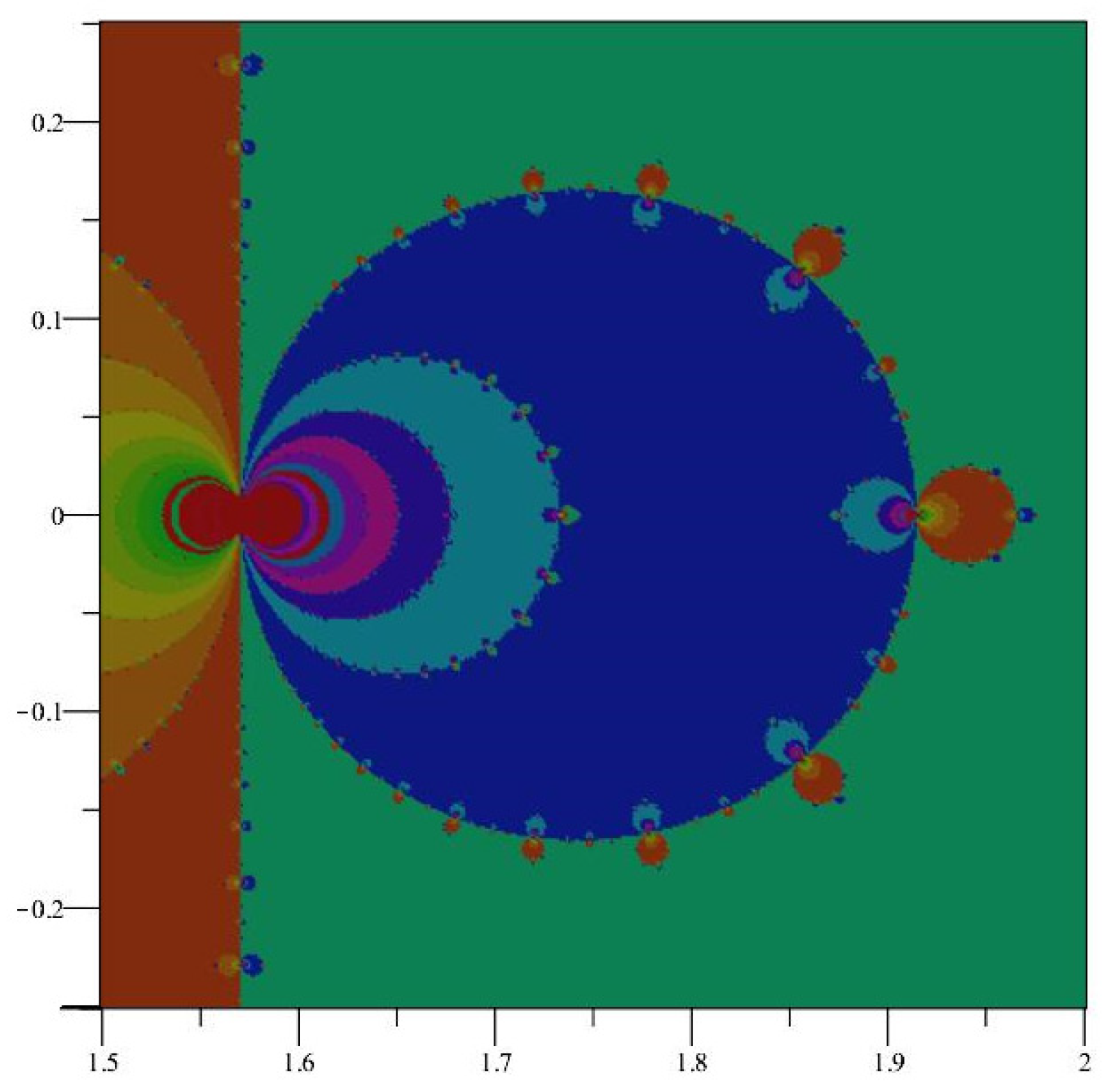
Because of the periodic nature of $\sin \left(z\right),$ the basins of attraction of iteration of $F_s$ appear periodic, with strips of width $\pi$ about each fixed point. See Figure 1. Points within each strip will generally converge to the root inside each strip, but not always. Indeed, we can see fractal behavior near the boundaries of the strips, and the dynamics here are decidedly non-trivial. Notice that the Newton map of $\sin \left(z\right)$ is not defined at $\frac{\pi }{2}+n\pi$, the zeros of $\cos \left(z\right),$ which produces the fractal boundary behavior shown in Figure 2. Further snapshots are displayed in Figure 3 and Figure 4, which are close-up images of the behavior of $F_s\left(z\right)$ near the singularities.

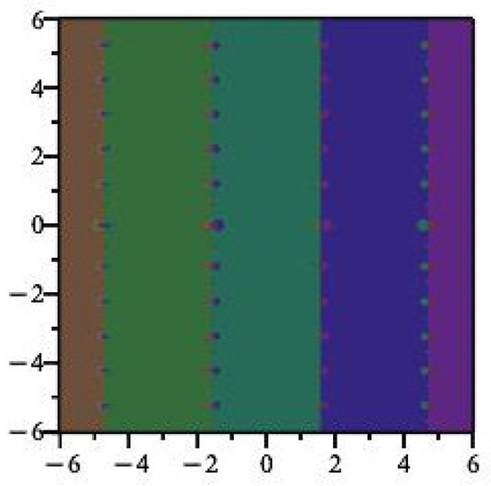
Figure 1. Dynamics of $F_s\left(z\right)$. Different colors represent different basins of attraction.

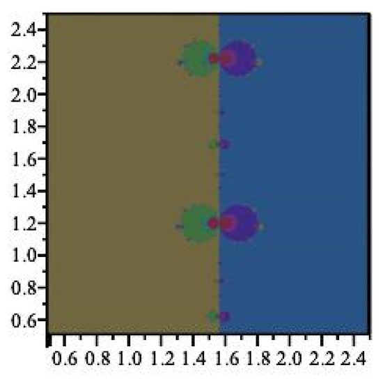
Figure 2. The fractal behavior of $F_s\left(z\right)$ at $z=\frac{\pi }{2}+iy$.

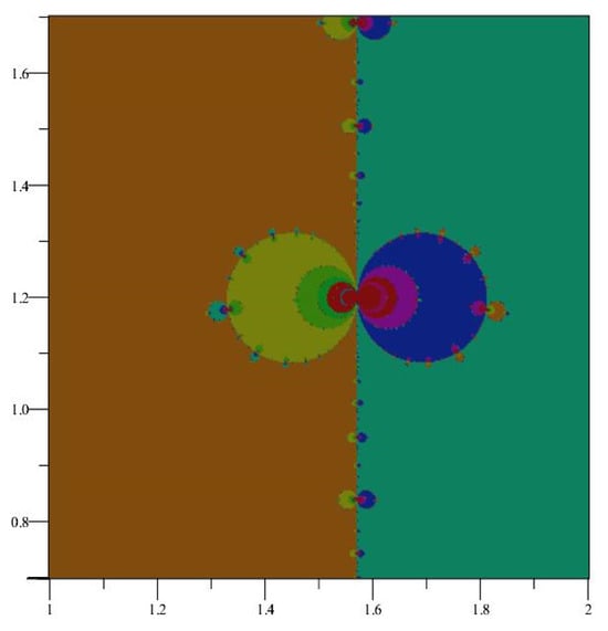
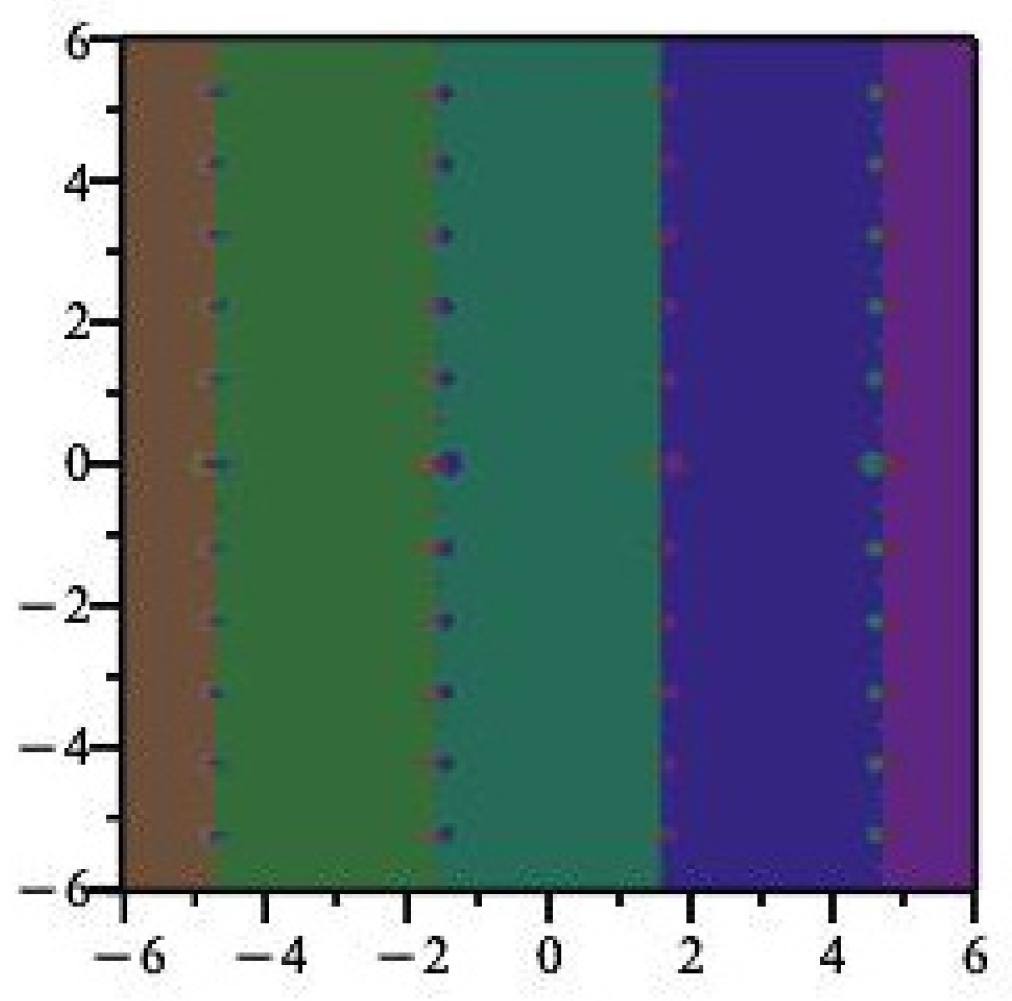
Figure 3. A closer view of the fractal behavior of $F_s\left(z\right)$ at $z=\frac{\pi }{2}+iy$.

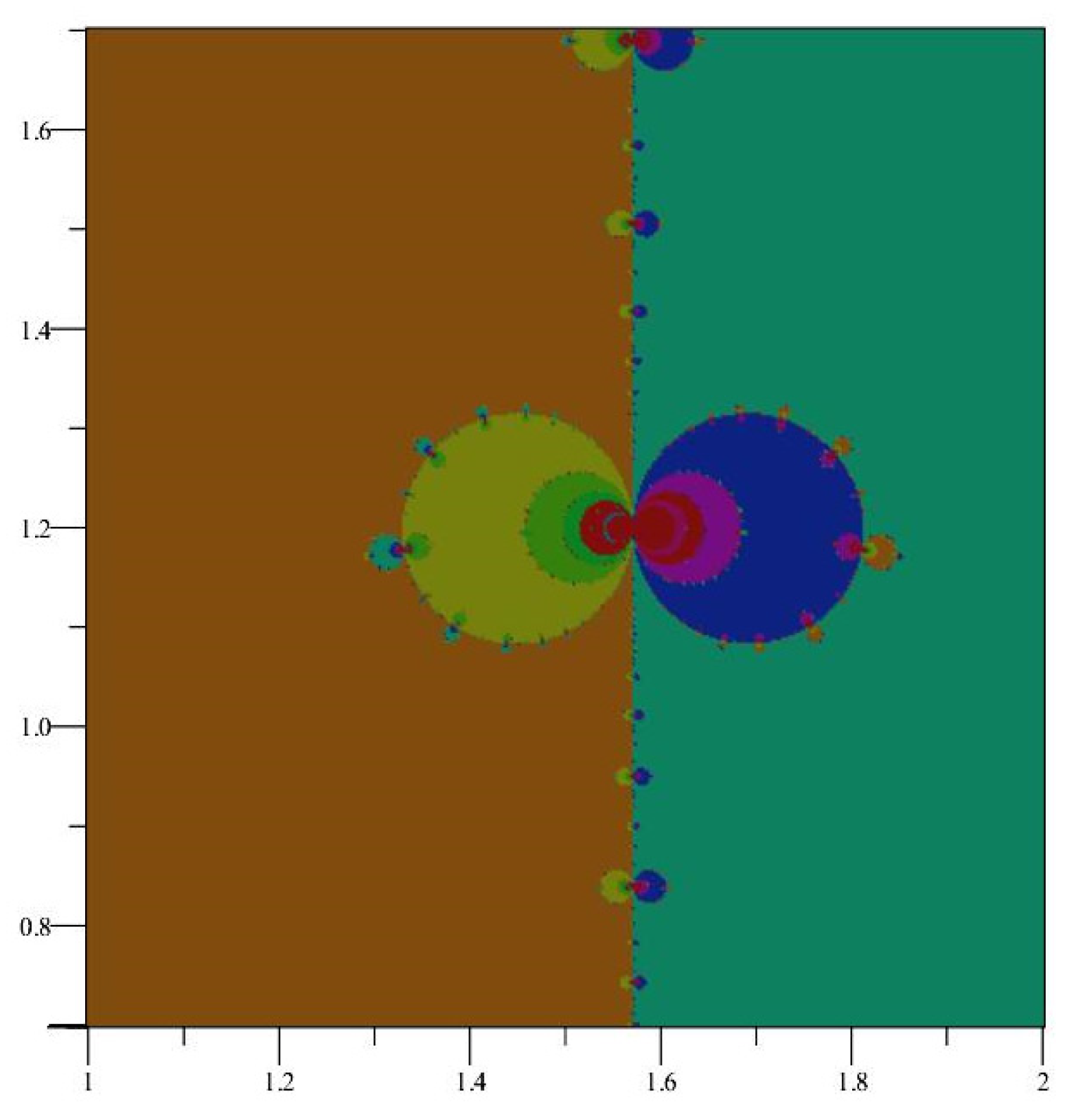
Figure 4. An even closer view of the fractal behavior of $F_s\left(z\right)$ at $z=\frac{\pi }{2}+iy$.

2.2. Symmetry of $F_s\left(z\right)$

We can begin to understand the symmetry that we observed in Figure 1 by recalling the following properties of the complex functions $\sin \left(z\right)$ and $\cos \left(z\right)$ [9,11]:

$$\sin \left(-z\right)=-\sin \left(z\right)$$

$$\cos \left(-\mathrm{z}\right)=\cos \left(\mathrm{z}\right).$$

$$\sin \left(\overline{\mathrm{z}}\right)=\overline{\sin \left(\mathrm{z}\right)}$$

$$\cos \left(\overline{\mathrm{z}}\right)=\overline{\cos \left(\mathrm{z}\right)}.$$

It follows easily that $F_s\left(z\right)$ is symmetric about the $x$-axis for all $z\in \mathbb{C}\left[4\right]$. If $F_s\left(z\right)=z-\frac{\sin \left(z\right)}{\cos \left(z\right)} ,$ then

$$\begin{gathered} F_s\left(\overline{z}\right)=\overline{z}-\frac{\sin \left(\overline{z}\right)}{\cos \left(\overline{z}\right)}=\overline{z}-\frac{\overline{\sin \left(z\right)}}{\overline{\cos \left(z\right)}}=\overline{z}-\overline{\frac{\sin \left(z\right)}{\cos \left(z\right)}} \\ =\overline{z-\frac{\sin \left(z\right)}{\cos \left(z\right)}}=\overline{z_1}= \overline{F_s\left(z\right)}. \end{gathered}$$

Similarly, $F_s(-\overline{z}$) = $-\overline{F_s\left(z\right)}$; hence, $F_s$ is symmetric about the $y$-axis.

This symmetry of $F_s$ means that we can restrict ourselves to an exploration of the dynamics that occur in the first quadrant to gain a full understanding of the global dynamics of $F_s$. See Figure 5.

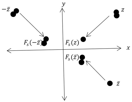
Figure 5. The x- and $y$-axis symmetry of $F_s\left(z\right)$.

Symmetry about the line $x=\pi$ (or any root of $\sin \left(z\right)$) also follows from the periodicity of $\mathrm{s}\mathrm{i}\mathrm{n}\left(z\right)$. If $F_s$ takes $z=x+iy$ to $z_1=x_1+i{y}_1,$ then it takes 2$\pi -\overline{z }=2\pi -x+iy$ to 2$\pi -\overline{z_1}=2\pi -x_1+i{y}_1$.

Finally, it can also be shown that there is symmetry about the line $x=\frac{\pi }{2}$ (or any vertical line midway between the vertical lines along the roots of sin(z)). Indeed, if $F_s$ takes $z=x+iy$ to $z_1=x_1+i{y}_1$, then it takes $\pi -\overline{z }=\pi -x+iy$ to $\pi -\overline{z_1}=2\pi -x_1+i{y}_1$.

2.3. Bounding the Primary Basins

We will now consider how we might construct some bounds on the basins of attraction of the fixed points $z_n=n\pi$. We also explore the implications of maintaining the condition that $|F_s\left(z\right)-z_n|<|z-z_n|.$

2.3.1. Bounds and Convergence along the x-Axis

Recall that the Newton map for $\sin \left(z\right)$ is $F_s\left(z\right)=z-\frac{\sin \left(z\right)}{\cos \left(z\right)}$. Since $\sin \left(x\right)$ and $\cos \left(x\right)$ are real for real values of $x$, then clearly, points on the real axis remain on the real axis under the iteration of $F_s$.

Since $z=0$ is a root of $\sin \left(z\right),$ and thus a fixed point of $F_s\left(z\right)$, let us begin our exploration by considering the behavior of $F_s\left(z\right)$ near 0. The primary basin of attraction of 0 will contain some real interval about 0, but how large can this interval be?

Consider the root $x^{\ast }\approx 1.166$ of $\frac{\sin \left(x\right)}{\cos \left(x\right)}-2x=0$ and notice

$$F_s\left(x^{\mathrm{*}}\right)=x^{\mathrm{*}}-\frac{\sin \left(x^{\mathrm{*}}\right)}{\cos \left(x^{\mathrm{*}}\right)}=x^{\mathrm{*}}-2x^{\mathrm{*}}=-x^{\mathrm{*}}$$

$$F_s\left({-x}^{\mathrm{*}}\right)=-x^{\mathrm{*}}-\frac{\sin \left({-x}^{\mathrm{*}}\right)}{\cos \left({-x}^{\mathrm{*}}\right)}=-x^{\mathrm{*}}+\frac{\sin \left(x^{\mathrm{*}}\right)}{\cos \left(x^{\mathrm{*}}\right)}=-x^{\mathrm{*}}+2x^{\mathrm{*}}=x^{\mathrm{*}}.$$

Thus, $x^{\ast }$ and $-x^{\ast }$ constitute a cycle of length 2, and we see the intersection of the primary basin of attraction of 0 with $\mathbb{R}$ cannot extend past $-x^{\ast }$ on the left and $x^{\ast }$ on the right.

Moreover, since $\frac{\sin \left(x\right)}{\cos \left(x\right)}>0$ on $\left(0,x^{\ast }\right),$ then for all $x\in (0,x^{\ast })$,

$$F_s\left(x\right)=x-\frac{\sin \left(x\right)}{\cos \left(x\right)}<x.$$

Next, notice that 2$x-\frac{\sin \left(x\right)}{\cos \left(x\right)}$ has zeros at $-x^{\ast }, 0,$ and $x^{\ast }$, is negative on $\left(-x^{\ast },0\right)$, and is positive on $\left(0,x^{\ast }\right)$. Thus, for all $x\in \left(0,x^{\ast }\right),$

$$0<2x-\frac{\sin \left(x\right)}{\cos \left(x\right)}$$

$$-x<x-\frac{\sin \left(x\right)}{\cos \left(x\right)}=F_s\left(x\right).$$

As a result,

$$\left|F_s\left(x\right)\right|<\left|x\right|$$

and every $x$ in $\left(0,x^{\ast }\right)$ does indeed move toward 0 under $F_s$.

By a similar argument (or simply relying on the symmetry of $\tan \left(x\right))$, we also see that every point in $\left(-x^{\ast },0\right)$ also moves toward 0 under $F_s$. Consequently, the intersection of $\mathbb{R}$ with the primary basin of attraction of 0 is precisely the interval $\left(-x^{\ast }, x^{\ast }\right)$.

The preceding analysis can be generalized to show, for all $n\in \mathbb{Z}$, that $F_s\left({n\pi -x}^{\ast }\right)$ = ${n\pi +x}^{\ast }$ and $F_s\left({n\pi +x}^{\ast }\right)$ = ${n\pi -x}^{\ast }$. Likewise, initial seed values in the range ${n\pi -x}^{\ast }<x<{n\pi +x}^{\ast }$ converge to the fixed point ${ z}_n=n\pi$.

2.3.2. Periodic Points along the x-Axis

We noted in the previous section that ${n\pi \pm x}^{\ast }$ constituted a cycle of period 2. We now consider more general periodic orbits.

The function $F_s$ maps the interval $\left(\left(n+\frac{1}{2}\right)\pi , {\left(n+1\right)\pi -x}^{\ast }\right)$ onto the interval (${\left(n+1\right)\pi +x}^{\ast }, \infty$) and maps the interval $\left({n\pi +x}^{\ast }, \left(n+\frac{1}{2}\right)\pi \right)$ onto the interval (${-\infty , n\pi -x}^{\ast })$. In fact, it appears that if we take any real point on the boundary of a basin of attraction for any fixed point, any neighborhood of that point contains points in the basins of attraction of all other fixed points.

For an integer j, define $I_j=[{j\pi +x}^{\mathrm{*}},{(j+1)\pi -x}^{\mathrm{*}}]$. Note that this interval contains $\left(j+\frac{1}{2}\right)\pi$. Then, $F_s\left(I_m\right)$ $\supset I_k$ for all $k\ne m$.

Let ${{\{a}_n\}}_{n=0}^{\mathrm{\infty }}$ be a sequence of integers such that $a_k\ne a_{k-1}$. Define $J_n=I_{a_n}$.

Define $Q_0=J_0$. Since $J_1\subset f\left(Q_0\right)$, $\exists Q_1\subset Q_0$ such that $f\left(Q_1\right)=J_1$.

Continuing, $J_2\subset f\left(J_1\right)=f\left(f\left(Q_1\right)\right),$ so there exists $Q_2\subset Q_1\subset Q_0$ such that $f\left(f\left(Q_2\right)\right)=f^2\left(Q_2\right)=J_2.$

By induction, we have $Q_n\subset Q_{n-1}\subset \cdots \subset Q_0$ such that $\forall k\le n,f^k\left(Q_k\right)=J_k$. Since $J_{n+1}\subset f\left(Q_n\right)$, we can continue the process and obtain $f^k\left(Q_k\right)=J_k\forall k=0,1,2,\cdots$

The intersection of nested closed sets is non-empty, so $\exists \tilde{x}$ $\in {\bigcap }_{k=0}^{\infty }{Q}_k$. $f^m\left(\tilde{x}\right)\mathcal{E}{J}_m \forall m=0, 1, 2, \cdots$

Stopping after a finite number, with the last integer the same as $a_j=a_0$, we have $f^j\left(Q_j\right)=J_j=J_0=Q_0$. Recall the one-dimensional version of Brouwer’s fixed point theorem, which states that any continuous function mapping a closed bounded interval to itself has a fixed point. Hence, for all j, $f^j$ has a fixed point, and we conclude that we have periodic orbits of all periods on the real axis. These results are related to those of Li and Yorke [12].

2.3.3. Bounds along Vertical Lines $x=n\pi$

Recall the standard identities, $\sin \left(z\right)=\frac{e^{iz}-e^{-iz}}{2i}$, and $\cos \left(z\right)=\frac{e^{iz}+e^{-iz}}{2}$, which gives

$$\sin \left(iz\right)=\frac{e^{-z}-e^z}{2i}, \mathrm{and} \cos \left(iz\right)=\frac{e^{-z}+e^z}{2},$$

Hence, for purely imaginary seed values,$z=bi$, $b\in \mathbb{R}$, we have $F_s\left(bi\right)=bi-\frac{\sin \left(bi\right)}{\cos \left(bi\right)}$ = $bi-i\frac{e^b-e^{-b}}{e^b+e^{-b}}$ = $i\left(b-\frac{e^b-e^{-b}}{e^b+e^{-b}}\right)$. Hence, all orbits that begin on the imaginary axis remain on that axis.

We can show that the imaginary axis is just a special case. Let us consider seed values on the vertical lines through the fixed points, that is, $z=n\pi +bi$, $n\in \mathbb{N},b\in \mathbb{R}$. Then, we have

$$\begin{gathered} F_s\left(n\pi +bi\right)=n\pi +bi-\frac{\sin \left(n\pi +bi\right)}{\cos \left(n\pi +bi\right)} \\ =n\pi +bi-\frac{\mathrm{s}\mathrm{i}\mathrm{n}\left(n\pi +bi\right)}{\mathrm{c}\mathrm{o}\mathrm{s}\left(n\pi +bi\right)}=n\pi +bi-\frac{\mathrm{s}\mathrm{i}\mathrm{n}\left(bi\right)}{\mathrm{c}\mathrm{o}\mathrm{s}\left(bi\right)} \\ =n\pi +bi-i\frac{e^b-e^{-b}}{e^b+e^{-b}}=n\pi +i\left(b-\frac{e^b-e^{-b}}{e^b+e^{-b}}\right). \end{gathered}$$

Hence, all orbits that begin on a vertical line through a fixed point remain on that line.

2.3.4. Convergence along Vertical Lines $x=n\pi$

The preceding calculations show that the convergence behavior along any of the vertical lines $x=n\pi$ is identical where $b$ is transformed to $b-\frac{e^b-e^{-b}}{e^b+e^{-b}}$ on each iteration.

We require that $⌊F_s\left(z\right)-z_n⌋<⌊z-z_n⌋.$ This means that we require $⌊F_s\left(n\pi +bi\right)-n\pi ⌋<⌊\left(n\pi +bi\right)-n\pi ⌋$ on the vertical lines:

$$⌊n\pi +i\left(b-\frac{e^b-e^{-b}}{e^b+e^{-b}}\right)-n\pi ⌋<⌊bi⌋$$

$$⌊i\left(b-\frac{e^b-e^{-b}}{e^b+e^{-b}}\right)⌋<⌊bi⌋$$

$$⌊b-\frac{e^b-e^{-b}}{e^b+e^{-b}}⌋<⌊b⌋$$

To verify this condition, we look at two cases.

The case of $b>0.$

Note that for $a,z\in \mathbb{R}$, if $0<a<z$, then $z-a<z$; hence, $|z-a|<\left|z\right|$. Therefore, we will prove that $0<\frac{e^b-e^{-b}}{e^b+e^{-b}}<b$. Clearly, $\frac{e^b-e^{-b}}{e^b+e^{-b}}>0$ for $b>0$.

To prove the second part of the inequality, we consider $I\left(b\right)=b-\frac{e^b-e^{-b}}{e^b+e^{-b}}$, and we note that $I\left(b\right)$ can be written as $b-Tanh\left(b\right)$.

It follows that $I^{\prime }\left(b\right)=1-(1-Tan{h}^2(b)$) = $Tan{h}^2\left(b\right)$). That means that $I^{\prime }\left(b\right)$ > 0, and $I\left(b\right)$ is an increasing function for $b>0$.

Since $I\left(0\right)$ = 0 and $I\left(b\right)$ is increasing for $b>0$, we deduce that $I\left(b\right)>0$ for $b>0$, that is, $b>\frac{e^b-e^{-b}}{e^b+e^{-b}},$ as required.

Since we have shown that $0<\frac{e^b-e^{-b}}{e^b+e^{-b}}<b,$ we can conclude that $⌊ b-\frac{e^b-e^{-b}}{e^b+e^{-b}}⌋<⌊b⌋,$ as required.

The case of $b<0.$

The development is analogous to that for $b>0.$

Note that for $a, z\in \mathbb{R}$, if $z<a<0$, then $z-a>z;$ hence, $|z-a|<\left|z\right|$. Therefore, we will prove that $b<\frac{e^b-e^{-b}}{e^b+e^{-b}}<0$. Clearly, $\frac{e^b-e^{-b}}{e^b+e^{-b}}<0$ for $b<0$.

In order to prove the second part of the inequality, we consider $I\left(b\right)=b-\frac{e^b-e^{-b}}{e^b+e^{-b}},$ and we note again that $I\left(b\right)$ can be written as $b-\mathrm{Tanh}\left(b\right)$.

It follows that $I^{\prime }\left(b\right)=1-(1-{{\mathrm{Tanh}}^2 \left(b\right)}^{ }$) = ${\mathrm{Tanh}}^2\left(b\right)$. That means that $I^{\prime }\left(b\right)$ > 0 and $I\left(b\right)$ is an increasing function for $b<0$.

Since $I\left(0\right)$ = 0 and $I\left(b\right)$ is increasing for $b<0$, we deduce that $I\left(b\right)<0$ for $b<0$, that is, $b<\frac{e^b-e^{-b}}{e^b+e^{-b}}$, as required. Since we have shown that $b<\frac{e^b-e^{-b}}{e^b+e^{-b}}<0$, we can conclude that $⌊ b-\frac{e^b-e^{-b}}{e^b+e^{-b}}⌋<⌊b⌋$, as required.

The preceding calculations have shown that convergence is monotone along the vertical lines that intersect the x-axis at the roots of $\sin \left(z\right)$.

2.3.5. Convergence in the Complex Plane

It was shown in Section 2.3.1 that points on the real axis $\left|x\right|<x^{\ast },$ where $x^{\ast }\cong 1.166,$ converge to the fixed point at 0. It appears numerically that the entire disk |z| < r $\cong 1.166$ is within the immediate basin of attraction.

Furthermore, the analysis in Section 2.3.2 shows that $x^{\ast }$ is a sharp bound on the immediate basin of attraction on the real axis. Hence, |z| < r $\cong 1.166$ is the largest possible disk centered at 0 in the immediate basin of attraction. This analysis can be extended to show that disks with the same radius surround all the fixed points of the Newton map of the Sine function.

For large values of Im(z), numerical simulations show that the Newton map behaves almost as $z=z-i sgn (Im (z\left)\right)$. As points approach the x-axis close to the singularity at $\left(n+\frac{1}{2}\right)\pi$, they are then projected off towards distant fixed points, as described in Section 2.3.2. This explains the general nature of the fractal behavior shown along the imaginary axis in Figure 1 and in the more refined image in Figure 4. It is illustrative of the chaotic nature of the Newton map how the behavior close to the imaginary axis is not uniform, as can be seen in the different sized bulbs shown in Figure 2 and Figure 3.

3. Comparison of Newton Maps of sin(z) and cos(z)

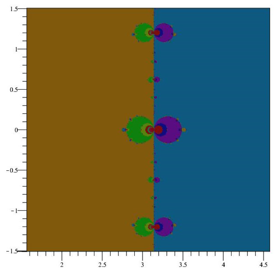
The images generated by iteration of the Newton map of the complex Cosine function $F_c\left(z\right)=z+$ $\frac{\cos \left(z\right)}{\mathrm{s}\mathrm{i}\mathrm{n}\left(z\right)}$ appear to be almost identical to those of the iteration of the Newton map of the complex Sine function, and some of those images are displayed in Figure 6, Figure 7 and Figure 8.

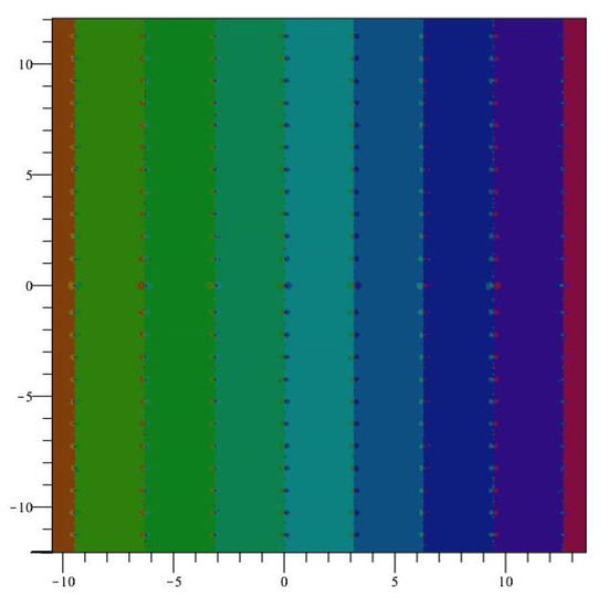
Figure 6. Global dynamics of $F_c\left(z\right)$.

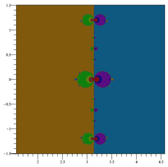
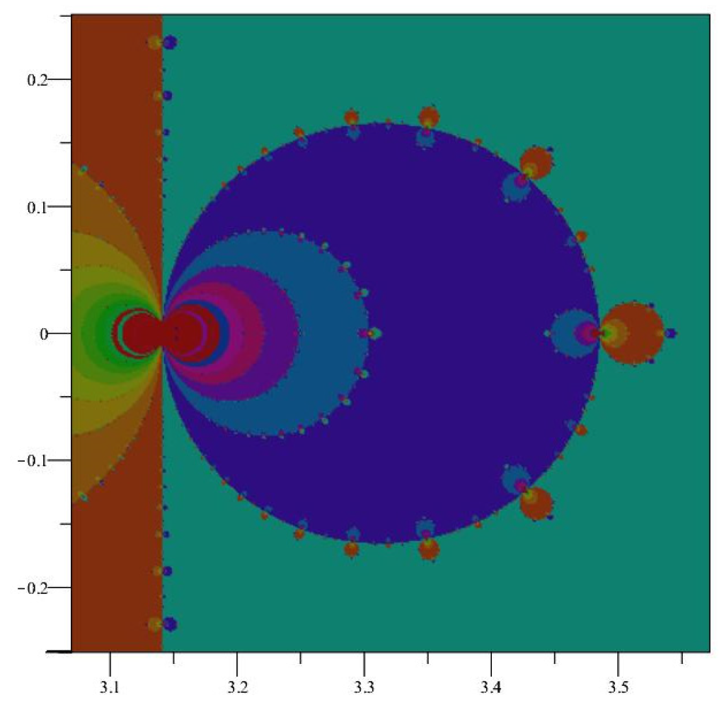
Figure 7. The fractal boundary of $F_c\left(z\right)$ at $z=\pi +iy$.

Figure 8. A closer view of the fractal boundary of $F_c\left(z\right)$ at $z=\pi +iy$.

These images can be compared with those for the Newton map of the complex Sine function shown in Figure 1, Figure 2, Figure 3 and Figure 4. The similarities should be expected, since $F_c\left(z+\frac{\pi }{2}\right)=z+\frac{\pi }{2}+$ $\frac{\cos \left(z+\frac{\pi }{2}\right) }{\sin \left(z+\frac{\pi }{2}\right) }$ = $z+\frac{\pi }{2}+$ $\frac{-\sin \left(z\right)}{\mathrm{c}\mathrm{o}\mathrm{s}\left(z\right)}$ = $F_s\left(z \right)+\frac{\pi }{2}$. In other words, an iteration of the Newton map of Cosine beginning at $z+\frac{\pi }{2}$ is identical to an iteration of the Newton map of Sine beginning at $z$ and then adding $\frac{\pi }{2}$.

4. Conclusions

The fractal image created from iterating the Newton map of $s\left(z\right)=\sin \left(z\right)$ is symmetric about both the $x$ and $y$ axes as well as with respect to each fixed point. In general, that which can be said about the dynamics surrounding $z_0=0$ can be said about the dynamics about $z_n=n\pi$. Indeed, we have shown monotonic convergence of all seed values on the x-axis close to the fixed points and on the vertical lines $x=n\pi$. More complicated behavior occurs close to the vertical lines $x=\left(n+\frac{1}{2}\right)\pi$.

References

- Gilbert, W. Newton’s Method for multiple roots. Comput. Graph. 1994, 18, 227–229. [Google Scholar] [CrossRef]
- Walsh, J. The Dynamics of Newton’s Method for Cubic Polynomials. Coll. Math. J. 1995, 26, 22–28. [Google Scholar] [CrossRef]
- Alexander, D.; Iavernaro, F.; Rosa, A. Early Days in Complex Dynamics: A History of Complex Dynamics in One Variable during 1906–1942; American Mathematical Society: Providence, RI, USA, 2012. [Google Scholar]
- Haeseler, F.; Peitgen, H. Newton’s method and complex dynamical systems. Acta Appl. Math. 1988, 13, 3–58. [Google Scholar] [CrossRef]
- Blanchard, P. The Dynamics of Newton’s Method. In Proceedings of the Symposia in Applied Mathematics, Cincinnati, OH, USA, January 1994; Complex Dynamical Systems: The Mathematics behind the Mandelbrot and Julia Sets. Devaney, R.L., Ed.; American Mathematical Society: Providence, RI, USA, 1994; Volume 49, pp. 139–154. [Google Scholar]
- Barnard, R.; Dwyer, J.; Williams, E.; Williams, G. Conjugacies of the Newton Maps of Rational Functions. Complex Var. Elliptic Equ. 2019, 64, 1666–1685. [Google Scholar] [CrossRef]
- Dwyer, J.; Barnard, R.; Cook, D.; Corte, J. Iteration of Complex Functions and Newton’s Method. Aust. Sr. Math. J. 2009, 23, 9–16. [Google Scholar]
- Bray, K.; Dwyer, J.; Barnard, R.; Williams, G. Fixed Points, Symmetries, and Bounds for Basins of Attraction of Complex Trigonometric Functions. Int. J. Math. Math. Sci. 2020, 2020, 1853467. [Google Scholar] [CrossRef]
- Saff, E.B.; Snider, A.D. Fundamentals of Complex Analysis for Mathematics, Science, and Engineering, 3rd ed.; Prentice Hall: Englewood Cliffs, NJ, USA, 2003. [Google Scholar]
- Stankewitz, R. Complex Dynamics: Chaos, Fractals, the Mandelbrot Set, and More. In Explorations in Complex Analysis; Mathematical Association of America: Washington, DC, USA, 2009. [Google Scholar]
- Conway, J. Functions of One Complex Variable I; Springer: New York, NY, USA, 1978. [Google Scholar]
- Li, T.Y.; Yorke, J.A. Period three implies chaos. Am. Math. Mon. 1975, 82, 985–992. [Google Scholar] [CrossRef]
Disclaimer/Publisher’s Note: The statements, opinions and data contained in all publications are solely those of the individual author(s) and contributor(s) and not of MDPI and/or the editor(s). MDPI and/or the editor(s) disclaim responsibility for any injury to people or property resulting from any ideas, methods, instructions or products referred to in the content. |
© 2024 by the authors. Licensee MDPI, Basel, Switzerland. This article is an open access article distributed under the terms and conditions of the Creative Commons Attribution (CC BY) license (https://creativecommons.org/licenses/by/4.0/).