Article

A Novel Method for Bearing Fault Diagnosis Based on a Parallel Deep Convolutional Neural Network

1
Leicester International Institute, Dalian University of Technology, Panjin 124221, China
2
School of Electrical Engineering, Dalian University of Technology, Dalian 116023, China
3
School of Automation, Guangdong University of Technology, Guangzhou 510006, China
4
School of Electrical and Electronic Engineering, Huazhong University of Science and Technology, Wuhan 430074, China
*
Author to whom correspondence should be addressed.
Symmetry 2024, 16(4), 432; https://doi.org/10.3390/sym16040432
Submission received: 29 February 2024 / Revised: 27 March 2024 / Accepted: 2 April 2024 / Published: 4 April 2024

Abstract

:
The symmetry of vibration signals collected from healthy machinery, which gradually degenerates with the development of faults, must be detected for timely diagnosis and prognosis. However, conventional methods may miss spatiotemporal relationships, struggle with varying sampling rates, and lack adaptability to changing loads and conditions, affecting diagnostic accuracy. A novel bearing fault diagnosis approach is proposed to address these issues, which integrates the Gramian angular field (GAF) transformation with a parallel deep convolutional neural network (DCNN). The crux of this method lies in the preprocessing of input signals, where sampling rate normalization is employed to minimize the effects of varying sampling rates on diagnostic outcomes. Subsequently, the processed signals undergo GAF transformation, converting them into an image format that effectively represents their spatiotemporal relationships in a two-dimensional space. These images serve as inputs to the parallel DCNN, facilitating feature extraction and fault classification through deep learning techniques and leading to improved generalization capabilities on test data. The proposed method achieves an overall accuracy of 96.96%, even in the absence of training data within the test set. Discussions are also conducted to quantify the effects of sampling rate normalization and model structures on diagnostic accuracy.

1. Introduction

1.1. Background and Scope

In the field of modern mechanical engineering, rolling bearings play a key role as essential components. However, the demands of high speeds, heavy loads, and extended operation in harsh environments make rolling bearings prone to various failures. Vibration signals that are collected from healthy machinery often exhibit strong symmetry. However, as the fault progresses, the symmetry of these signals gradually deteriorates. Failing to promptly identify asymmetry in the signal can lead to a series of consequences, including reduced bearing performance, shortened lifespan, and potentially catastrophic system failures [1]. Accurate and timely fault diagnosis is paramount, given the importance of rolling bearings to overall system performance and safety [2]. Unfortunately, the signals detected from rolling bearings are often obscured by background noise and extraneous information, making accurate and reliable diagnosis challenging. Therefore, continuous research and development efforts are needed to enhance fault diagnosis techniques further and ensure the optimal performance and safety of mechanical systems that rely on rolling bearings [3].
Currently, fault diagnosis for rolling bearings involves two main approaches: traditional time-frequency analysis methods and emerging AI-based techniques. Traditional methods rely on established signal processing techniques to extract fault signatures from noisy backgrounds. In contrast, AI-based techniques leverage pattern recognition and predictive capabilities to improve diagnostic accuracy and precision. These two approaches provide a comprehensive solution for fault diagnosis in rolling bearings, leading to more resilient and reliable mechanical systems.

1.2. Related Works

Currently, numerous time-frequency domain analysis methods are widely applied. These methods either directly extract or reconstruct signaling components in the time domain, often relying on specific iterative algorithms or model optimization techniques to achieve effective signal decomposition, or they adopt techniques such as wavelet transforms, which essentially employ filtering methods aimed at extracting waveform information of different frequencies from the signal. Among them, empirical mode decomposition (EMD) is currently the most prominent signal decomposition method [4]. However, EMD also presents numerous challenges, such as boundary effects, mode mixing, sensitivity to noise, and a lack of mathematical theoretical support. To address these issues, the authors of [5] proposed ensemble empirical mode decomposition (EEMD), which eliminates the mode mixing problem. Many researchers in these areas have proposed methods such as cosine filter-based empirical mode decomposition [6], B-spline-based approaches to enhance EMD performance [7], and replacement-selection algorithm-based methods [8]. These advancements have significantly improved the accuracy of time-domain signal decomposition and the precision of bearing fault diagnosis. Similar to EMD, iterative filtering decomposition (IFD) is a method that utilizes low-pass filtering techniques to obtain the mean value of the signal, ensuring better convergence [9]. To address the issue of frequency mixing, adaptive local iterative filtering methods were introduced in [10]. These methods adaptively adjust the filter length at different time instances, enabling the decomposition of frequency-modulated signaling components and achieving promising results.
During bearing faults, prominent non-stationary signals often accompany the detected waveforms, and the direct application of the aforementioned transforms in such scenarios yields unsatisfactory results. Many studies have investigated the nonlinear frequency modulation characteristics of signaling components by extensively exploring new theories and methods for nonlinear frequency modulation component decomposition. This has led to significant improvements in the accuracy of bearing fault diagnosis. Reference [11] introduces an enhanced NSP algorithm based on complex-valued differential operators for multi-component signal separation, which exhibits quadratic convergence and superior performance compared to other advanced methods. The authors of [12] presented a variational approach for nonlinear chirp mode decomposition, which works on scale-space representation-based automated boundary detection in a magnitude spectrum. One study [13] addressed the limitations of existing signal decomposition methods by introducing adaptive bandwidth parameters, and it has been successfully applied in mechanical fault diagnosis. Furthermore, methods such as those based on ridge path regrouping and intrinsic chirp component decomposition [14], parameterized time-frequency transforms and phase compensation techniques [15], and rough time-frequency ridge-guided multi-band feature extraction [16] have demonstrated precise extraction capabilities for non-stationary signals, significantly facilitating accurate bearing fault diagnosis.
The advent of deep learning theories has profoundly impacted bearing fault diagnosis. Deep learning excels at extracting features from high-dimensional data, offering strong generalizability and robustness [17]. Recently, researchers have found that mapping time-domain signals to the time-frequency domain via TFA methods before applying deep learning can lead to better outcomes. TFA techniques range from conventional (e.g., Fourier and wavelet transform) [18,19,20] to advanced methods (e.g., transient-extracting transform and synchrosqueezing transform) [3,21,22], all providing valuable foundations for deep learning-based fault diagnosis. For the deep learning-based method, the authors [23] introduced an advanced CNN for bearing fault diagnosis, integrating signal processing and deep learning for precise feature extraction and classification, outperforming traditional methods. The authors of [24] presented a tailored HADCNN for bearing faults, which significantly boosted identification accuracy. In [25], a robust deep-learning model was used to handle raw vibration signals and achieved excellent results in noisy environments without complex feature engineering. Another study [26] surveyed deep learning techniques for bearing fault diagnosis and analyzed their strengths, limitations, and areas for improvement. The authors of [27] enhanced deep learning for rotating machinery faults using data augmentation, improving classification accuracy, especially with limited data. The aforementioned deep learning algorithms have achieved profound impacts, with numerous studies demonstrating their robust capabilities in accurately identifying the types and severity of bearing faults. This approach effectively enhances diagnostic reliability and provides valuable support for the health monitoring and maintenance of mechanical equipment. Similar approaches have demonstrated marked effectiveness in various areas. For instance, the study in [28] extracted useful features from local current signals to generate RGB images for utilization by a CNN classifier. Furthermore, the research conducted in [29] initially employed variational mode decomposition to extract pertinent features from locally measured current signals, subsequently feeding them into a deep CNN for efficient fault detection and classification in transmission lines. These examples clearly demonstrate the powerful capabilities of deep learning methods in addressing fault identification, diagnosis, and classification issues.

1.3. Motivation

Despite the remarkable achievements of deep learning algorithms in bearing fault diagnosis, there are still several pressing issues in this domain:
(1)
First, the current time-frequency domain analysis methods combined with deep learning algorithms exhibit limitations in capturing the spatiotemporal relationships between sampling points in input time series, which constrains the accuracy of diagnostic outcomes. Specifically, when dealing with complex and nonlinear bearing fault signals, these methods often struggle to adequately reveal the underlying structure and dynamic characteristics of the signals, thereby affecting the precision and reliability of the diagnosis.
(2)
Second, deep learning models tend to produce biased diagnostic results when the input time series sampling rate differs from that of the training data. This indicates a need to enhance the model’s ability to extract features and recognize patterns under varying sampling rates. Unfortunately, research addressing this issue is insufficient, and practical solutions have not yet been proposed to optimize model performance across different sampling rates.
(3)
Finally, the generalization capability of deep learning models poses a significant challenge. In practical applications, models often perform well on training data collected under specific load conditions. However, when the load conditions change, and the current load scenario is not included in the training set, the diagnostic accuracy decreases, highlighting the model’s limitations in adapting to different operating conditions and load variations.
When these three issues occur simultaneously, using deep learning methods for bearing fault diagnosis faces even more complex and challenging obstacles.

1.4. Contributions

To address the aforementioned issues, this paper proposes a bearing fault diagnosis method based on integrating the Gramian angular field (GAF) and parallel deep convolutional neural network (DCNN), aiming to address all three problems simultaneously. The following contributions correspond to the motivations for this study:
(1)
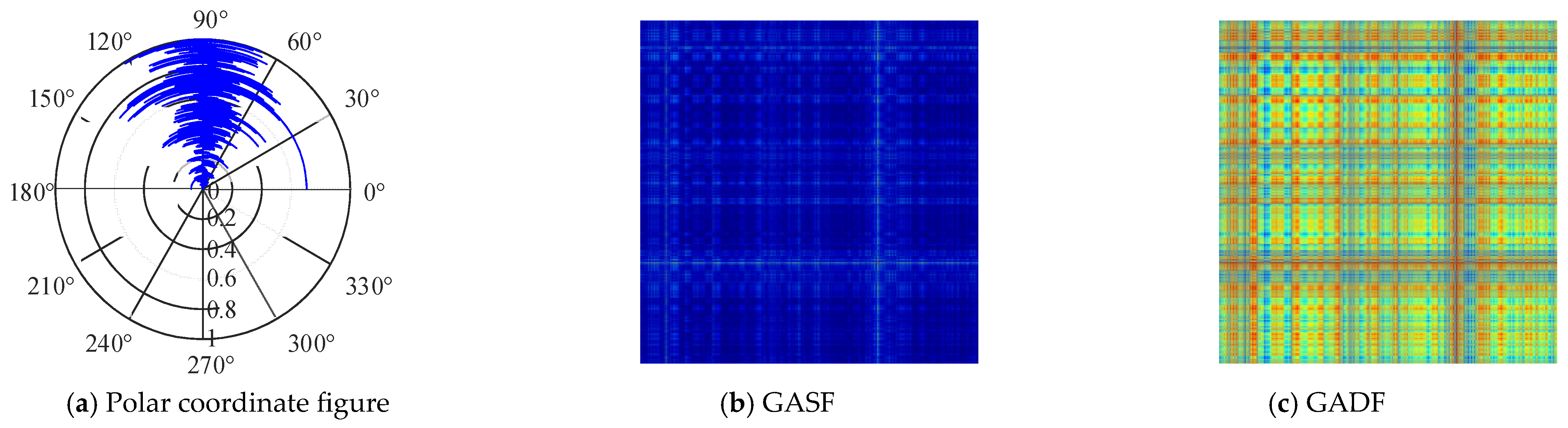
First, we employed the GAF to convert the waveforms obtained under various bearing operating conditions at specific sampling frequencies into images, generating a set of Gramian angular summation field (GASF) and Gramian angular difference field (GADF) images through the GAF transformation. Both GASF and GADF simultaneously calculate the spatiotemporal correlations between sampled sequence points in polar coordinates, effectively mitigating common-mode and differential-mode interference in the signals.
(2)
Second, we delve into data preprocessing techniques when the sampling rate of the input time series differs from that of the training data. It introduces an upsampling method for input samples based on cubic spline interpolation, further enhancing the accuracy of diagnostic results. Detailed experimental results are provided to support this approach.
(3)
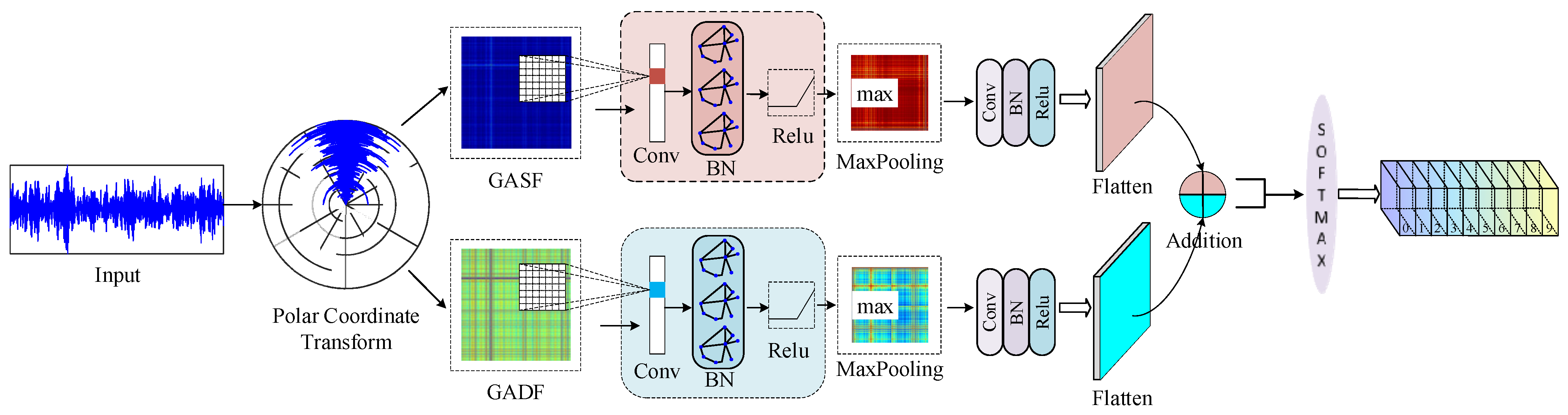
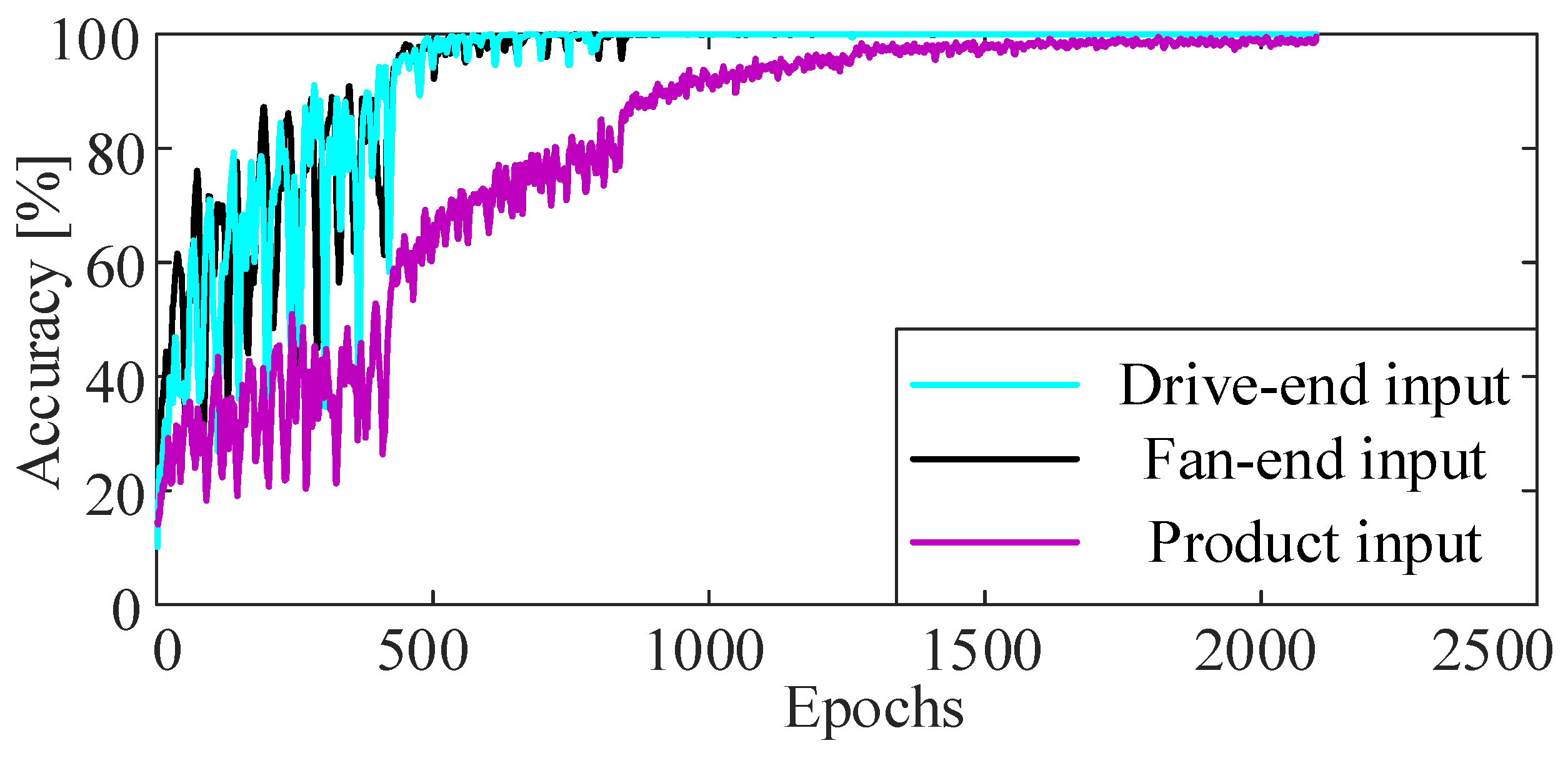
Finally, we present a parallel DCNN-based method for bearing fault diagnosis. Each CNN within the parallel DCNN comprises two convolutional layers designed to extract vibration patterns under different operating conditions as comprehensively as possible. These networks process the image data generated by GASF and GADF separately. An attention mechanism is then employed to fuse the features extracted by the two CNNs, culminating in a comprehensive fault diagnosis methodology. The experimental results demonstrate that this approach exhibits strong adaptability to varying load conditions.
The remainder of this paper is organized as follows. In Section 2, a theoretical analysis is conducted to introduce the data preprocessing methodology, including the upsampling method, the GAF transform, the establishment of the parallel DCNN, and the attention mechanism to consider both the GASF and the GADF channels. In Section 3, case studies are conducted to assess the performance of the proposed method under various fault scenarios. The performance of the method is quantified using several indicators. In Section 4, the necessity of sampling rate normalization and the superiority of the proposed method over existing methods are validated. Section 5 discusses the method’s robustness in scenarios involving large sample sizes and repetitive trials. The optimal model structure is also discussed.

2. Theoretical Basis and Methodology

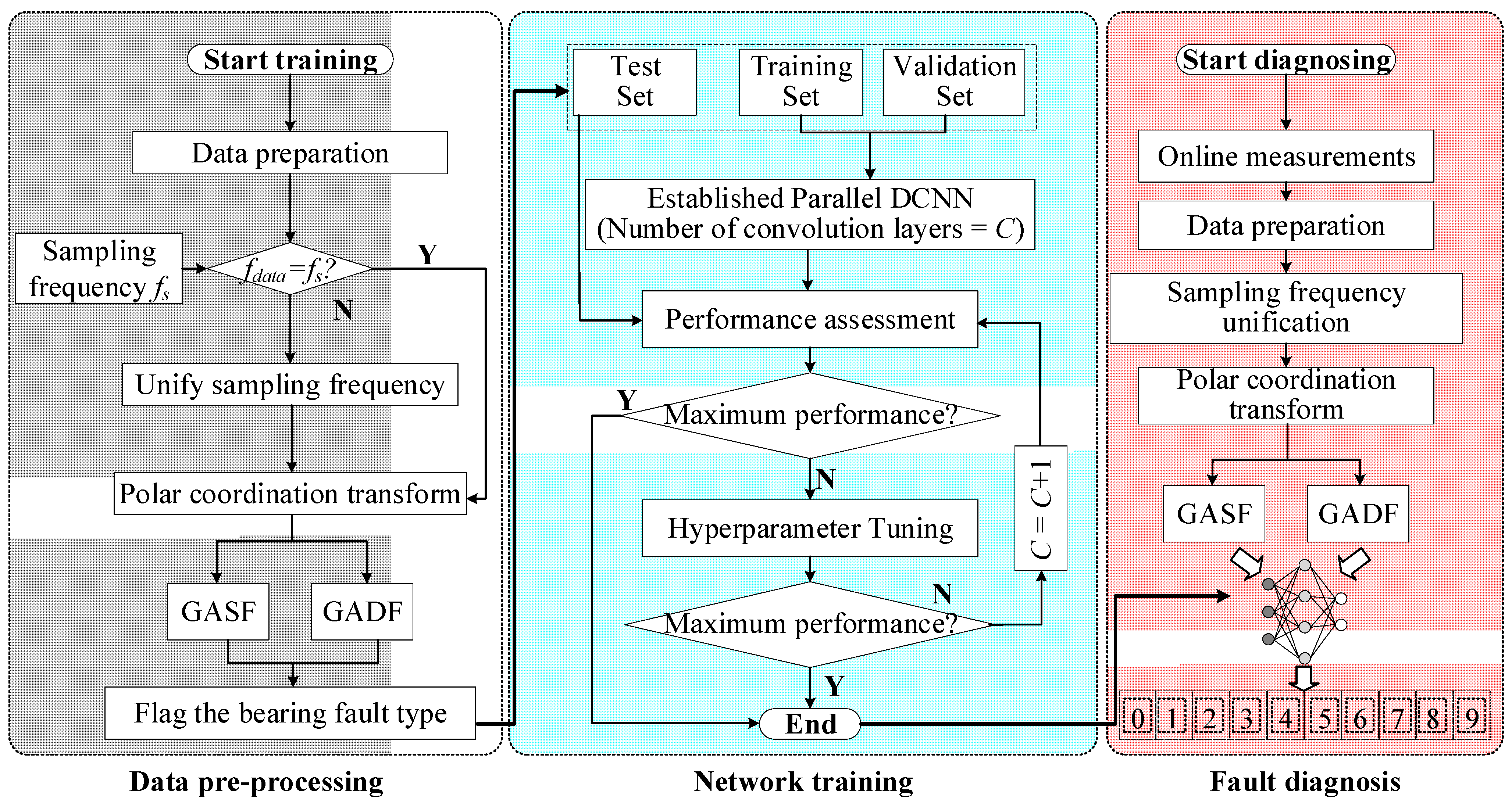
2.1. Data Preprocessing

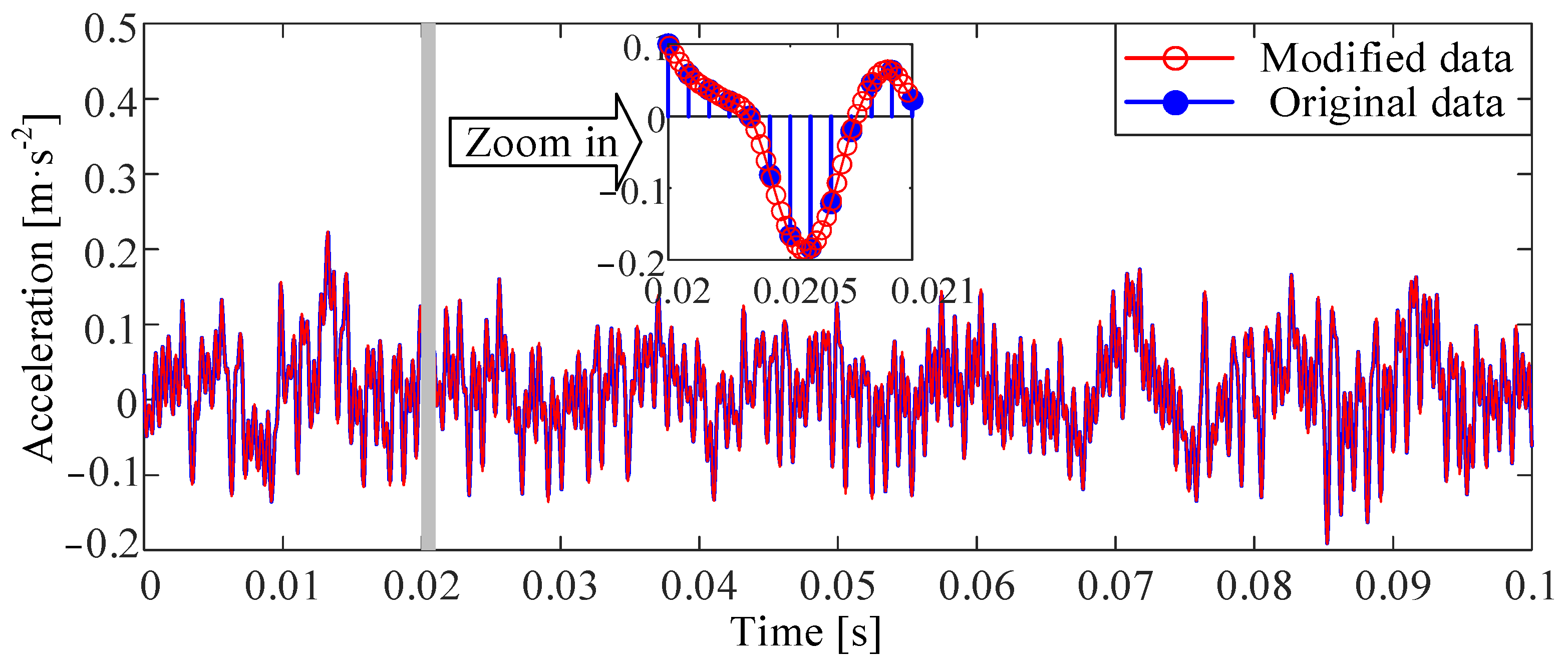
2.1.1. Sampling Rate Normalization

In terms of varying load scenarios, rolling bearing failures can be broadly categorized into four distinct modes: normal operation, inner ring defects, outer ring defects, and rolling element defects, as shown in Figure 1. Each of these modes exhibits varying degrees of degradation. A critical challenge arises because, even within the same mechanical system, different experimental settings often necessitate the use of diverse sampling rates. This inconsistency in sampling rates poses a significant obstacle to the reliable extraction of fault features from rolling bearings under identical fault conditions.
To ensure consistent feature extraction across different scenarios, it is imperative to preprocess the sampled data and harmonize their dimensions. This preprocessing step involves normalizing the data to a common format or standard, facilitating accurate comparisons and analyses. To unify the feature dimensions, these sampling results must be preprocessed. Assuming that a signal collected from a rolling bearing is represented as:
x = ( u + n ) h
where x, u, n, and h are the sampled signal, impulsive signal of the faulty bearing, background noise, and convolution of the transmission path, respectively. Let fs denote the sampling rate and x = { x [ 1 ] , x [ 2 ] , x [ i ] , x [ n ] } be the sampled signal sequence represented accordingly. Given an upsampling factor L, the new sampling rate after upsampling should be Lfs. The fundamental principle behind upsampling using cubic spline interpolation [30] is as follows:
First, each sample point in the original sampling sequence x is treated as an interpolation node. These nodes serve as control points for constructing the cubic spline interpolation function. Then, for each pair of adjacent interpolation nodes (x[i]) and (x[i + 1]), a cubic polynomial (Sn(t)) is constructed. Here, t is a normalized time variable that varies between 0 and 1. The general form of this polynomial expression is:
S i ( t ) = a i + b i t + c i t 2 + d i t 3
where ai, bi, ci, and di are the coefficients of the polynomial, which need to be determined based on the function values, first derivatives, and second derivatives at nodes (x[i]) and (x[i + 1]). They can be obtained by solving a system of linear equations subject to the following boundary conditions:
  • The boundary conditions for the equality of acquired signal values are as follows:
{ x [ i ] = S i ( t ) | t = 0 x [ i + 1 ] = S i ( t ) | t = 1
2.
The boundary conditions for the equality of the first derivatives of the acquired signals are as follows:
{ x ˙ [ i ] = S i ( t ) | t = 0 x ˙ [ i + 1 ] = S i ( t ) | t = 1
3.
The boundary conditions for the equality of the second derivatives of the acquired signals are as follows:
{ x ¨ [ i ] = S i ( t ) | t = 0 x ¨ [ i + 1 ] = S i ( t ) | t = 1
By utilizing the tridiagonal matrix algorithm [31] to solve Equations (1)–(5), the unification of sampling rates for fault acquisition signals of rolling bearings under different sampling rates can be achieved. Denoting this unified signal as y, the correspondence relationship between the signals before and after the upsampling operation is as follows:
y = [ y [ 1 ] , y [ 2 ] , y [ n L ] ]
In Equation (6), we have:
{ y [ j L L + 1 ] = x [ j ] , j = 1 , 2 , , n y [ j L L + 2 ] = S j ( t ) | t = j + 1 / L , j 1 , 2 , , n y [ j L ] = S j ( t ) | t = j + ( L 1 ) / L j 1 , 2 , , n

2.1.2. Visualization of the Input Time Series

GAF is a methodology that facilitates the transformation of time series data into image-based representations [32]. This approach not only preserves the integrity of the signal information but also maintains the temporal dependencies inherent in the original one-dimensional sampled sequence. Initially, the GAF resales the time series data within a specified range. Subsequently, each time point’s value is converted into an angular representation by computing the polar coordinates of the rescaled time series. Finally, the GAF derives two distinct fields: the Gramian angular summation field (GASF), which calculates the cosine of the sum of all the angles, and the Gramian angular difference field (GADF), which determines the sine of the same summation. This conversion results in an image where each pixel’s value corresponds to a specific time point in the original data. The advantage of this process is that the resulting images are highly suitable as input for image processing models, such as convolutional neural networks, which were previously inapplicable to time series data in their raw form. First, the rolling bearing fault signal y, obtained under unified sampling rate conditions, undergoes normalization and scaling as follows:
y ¯ i = 2 ( y i min ( y ) ) max ( y ) min ( y ) 1
To capture the spatiotemporal relationships between the normalized sequence points obtained from Equation (8), the sequence can be represented using the amplitude and phase angle in polar coordinates:
{ ϕ i = arccos ( y ¯ i ) , 1 y ¯ i 1 , y ¯ i y r i = t i / N ( y ) , t i = 1 , 2 , , N ( y )
The length of the normalization matrix, denoted by N(y), is equivalent to nL in this paper. Each normalized timestamp ti within the sequence is associated with a distinct phase angle ϕ i . This association implies that, over time, a particular time series will follow a consistent and distinguishable pattern in polar coordinates. Consequently, by calculating both the sum and difference of angles for every pair of points, we can derive two matrices: the GASF and the GADF. These matrices serve to quantitatively represent the temporal relationships between sample values at varying time intervals within the same time series, providing a comprehensive characterization of its internal dynamics:
G GASF = [ cos ( ϕ 1 + ϕ 1 ) cos ( ϕ 1 + ϕ 2 ) cos ( ϕ 1 + ϕ n L ) cos ( ϕ 2 + ϕ 1 ) cos ( ϕ 2 + ϕ 2 ) cos ( ϕ 2 + ϕ n L ) cos ( ϕ n L + ϕ 1 ) cos ( ϕ n L + ϕ 2 ) cos ( ϕ n L + ϕ n L ) ] = y ¯ T y ¯ 1 y ¯ 2 T 1 y ¯ 2
G GADF = [ sin ( ϕ 1 ϕ 1 ) sin ( ϕ 1 ϕ 2 ) sin ( ϕ 1 ϕ n L ) sin ( ϕ 2 ϕ 1 ) sin ( ϕ 2 ϕ 2 ) sin ( ϕ 2 ϕ n L ) sin ( ϕ n L ϕ 1 ) sin ( ϕ n L ϕ 2 ) sin ( ϕ n L ϕ n L ) ] = 1 y ¯ 2 T y ¯ y ¯ T 1 y ¯ 2
It is evident that for the same input time series, GASF and GADF can be utilized to mitigate differential mode interference and common mode interference, respectively. This significantly contributes to enhancing the robustness of fault diagnosis.

2.2. Fault Diagnosis Based on a Parallel Deep Convolutional Neural Network

The parallel DCNN is a sophisticated deep learning architecture designed for accelerated performance through parallel computing techniques. At its core, it encompasses an intricate hierarchy of layers, including an input layer, multiple convolutional layers for feature extraction, pooling layers for downsampling, fully connected layers for high-level reasoning, and an output layer for final predictions. Within this framework, the layers operate seamlessly, leveraging the power of parallel processing to handle data concurrently and expedite model training. This parallelization aspect is crucial in addressing the computational demands of complex pattern recognition tasks.
In the context of this study, Figure 2 outlines the architecture of the employed parallel DCNN model. The workflow commences with the preprocessing of input data through a polar coordinate transformation. This transformation, governed by Equation (9), reveals the temporal evolution of phases, encoding valuable information for subsequent analysis. Subsequently, the transformed data undergo further refinement through the computation of the GASF and GADF, as dictated by Equations (10) and (11), respectively. These calculations capture angular relationships and differences within the data, enriching the feature set available to the model. Finally, the enriched data, which are now encoded with both spatial and temporal characteristics, are fed into the parallel DCNN. Herein, the model leverages its parallel processing capabilities to process the data and learn intricate patterns.

2.2.1. Selection Principle for the Input Data Length

The selection of the input data length, denoted by the parameter nL mentioned earlier, requires careful consideration of the characteristic frequencies across various fault modes. This ensures that the input data are sufficiently long to reliably capture the distinctive oscillatory patterns associated with different types of faults. However, excessively long data can undermine the real-time capability of the proposed method, potentially complicate input features, and reduce training efficiency. As indicated in [33], for bearings with a fixed outer ring installation, the characteristic frequencies include the ball-pass frequency of the inner ring (BPFI), the ball-pass frequency of the outer ring (BPFO), and the rolling element rotational frequency (BEF), which are calculated as follows:
f BPFI = 1 2 z f i ( 1 + d D cos α )
f BPFO = 1 2 z f i ( 1 d D cos α )
f BEF = 1 2 D d ( 1 d 2 D 2 cos 2 α ) f i
where fi is the rotational frequency of the inner ring in r/s. D and d are the pitch diameter and the rolling element diameter, respectively. α is the contact angle. Let fre be the maximum resolution frequency. The following equation is used:
L f s × T w = n L
where Tw is the window length corresponding to the maximum resolution frequency, and Tw = 1/fre. The maximum resolution frequency is determined as the greatest common divisor (GCD) of BPFI, BPFO, and BEF:
f r e = G C D ( f B P F I , f B P F O , f B E F )
Substituting Equations (15) and (16), we have the value of n:
n = f s G C D ( f B P F I , f B P F O , f B E F )
where [[ ]] represents the rounding operator.

2.2.2. Structure and Parameter Determination of the Parallel DCNN

The dual-channel CNNs include convolutional layers, batch normalization (BN) layers, rectified linear unit (ReLU) layers, and max pooling layers. The convolutional layer extracts local features from the input data via convolutional operations. Each convolutional layer comprises multiple convolution kernels that slide over the input data, executing convolutional operations to generate feature maps. These maps are then stacked, enabling the progressive extraction of increasingly abstract and intricate features. When confronted with intricate input features, the deployment of multiple convolutional layers bolsters the network’s comprehension of complex input samples. Specifically, in this investigation, two convolutional layers are dedicated to extracting features from the GASF and GADF images, with dimensions of 7 × 7 and 3 × 3, respectively.
The pooling layer, situated subsequent to the convolutional layer, serves to diminish the dimensionality of the feature maps. This reduction not only alleviates computational demands but also mitigates the risk of overfitting; in this endeavor, max pooling is the chosen method. Following the ReLU layer, two fully connected layers of identical dimensions are positioned, amalgamating the ultimate convolutional outputs for holistic feature learning and classification. These layers foster dense connections. Notably, in this endeavor, the DCNN does not directly yield classification outcomes. Instead, it employs an attention mechanism to amalgamate features from GASF and GADF. Consequently, the flattened layer is situated subsequent to the fully connected layers. In the context of this investigation, the fully connected layers for both the GASF and GADF pathways are configured with 128 neurons.
Furthermore, within the parallel DCNN architecture established in this study, an additional layer is positioned after the two flattened layers. Subsequently, a self-attention layer is introduced to compute attention weights pertaining to each element vis-à-vis other elements within the two sequences. These weights are indicative of the significance of distinct elements in decision-making processes. Specifically, each element within the sequences emanating from the GASF and GADF flattened layers is assigned a query vector, a key vector, or a value vector. The query vector facilitates the computation of matching scores with the key vectors, while the value vectors underlie the calculation of weighted sums to arrive at the final output. By leveraging the self-attention layer, the model gains enhanced flexibility in processing information within the input sequences, enabling it to prioritize the most pertinent aspects pertinent to the task at hand. This mechanism proves particularly advantageous in managing variable-length sequences, capturing intricate dependencies within sequences, and tackling complex tasks, thus justifying its application in this study.
Additionally, the output generated by the self-attention layer undergoes further processing via a fully connected layer and is transformed into a probability distribution using the Softmax function. This yields predicted probabilities for each of the ten classes pertaining to bearing operating conditions, as delineated in Table 1.

2.2.3. Methodology

The bearing fault diagnosis process based on the parallel DCNN, as depicted in Figure 3, comprises three stages: data preprocessing, network training, and real-time diagnosis. The details are as follows:
  • Data preprocessing: Obtain the bearing fault waveforms and specify the sampling rate for the waveforms used in training. If a portion of the waveforms in the training samples has a different sampling rate from the others, the method described in this paper is employed to perform upsampling using cubic spline interpolation. Following polar coordinate transformation, the vibration signal sample set undergoes GAF transformation, converting the one-dimensional time series data into two-dimensional GASF and GADF images. These training samples are then labeled according to their operational conditions using the method outlined in Table 1 to distinguish between different abnormal or normal states.
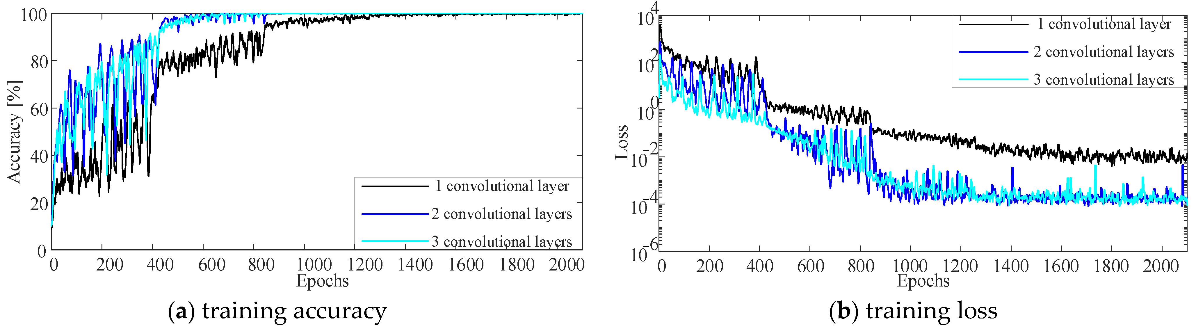
  • Network training and validation: The labeled image data are divided into training, validation, and test sets. The parallel DCNN model is used for training, and the model’s performance is validated using the validation set during each iteration. When the model meets the preset convergence criteria, the model parameters are saved. Notably, if satisfactory performance cannot be achieved or training does not converge despite hyperparameter adjustments, the number of convolutional layers is increased by 1, and the hyperparameter adjustment process is repeated until satisfactory diagnostic performance is obtained.
  • Fault diagnosis: During the actual operation of the system, the vibration signals of the bearings are collected in real-time. After adjusting the sampling rate and undergoing polar coordinate transformation, the GASF and GADF images are generated. These images are then input into the trained model to monitor the operational health status of the bearings in real-time.
Figure 3. A flowchart of the fault diagnosis methodology.
Symmetry 16 00432 g003

3. Results

This paper utilizes experimental rolling bearing data obtained from the Electrical Engineering Laboratory at Case Western Reserve University in the United States. The experimental setup, as depicted in Figure 4a, involves a connection between a motor and a load via a transmission shaft, with the SKF6205 deep groove ball bearing positioned at the motor’s drive end. Vibration signals are acquired using a 16-channel data recorder at sampling frequencies of 12 kHz and 48 kHz. These signals encompass data from both the fan-end and drive-end sensors, including normal baseline data, drive-end bearing fault data, and fan-end bearing fault data [34,35].
The experiments are conducted under varying loads and rotational speeds, encompassing ten distinct states of the rolling bearing, including normal operation, inner race faults, outer race faults, and ball faults, each with different levels of performance degradation. Data from the drive end, sampled at 48 kHz, are selected for analysis. The fault conditions are distinguished by the damage diameters on the inner race (IR), balls (B), and outer race (OR), with suffixes 07, 14, and 21 denoting damage severities of 7 mils, 14 mils, and 21 mils, respectively; N denotes the normal state.
The experiments are performed under four different loads: 0 hp, 1 hp, 2 hp, and 3 hp. To assess the model’s generalization capabilities across various loads, data from the 1 hp, 2 hp, and 3 hp loads are used as the training set, while data from the 0 hp load serve as the test set. The method for generating the datasets involves segmenting the data using a fixed-size window, as illustrated in Figure 4b, and then moving the window by a x% step size to capture the next segment.
Utilizing data from [35], the experimental bearing parameters are determined as follows: pitch diameter D = 39.0398 mm, rolling element diameter d = 7.94004 mm, number of rolling elements z = 9, contact angle α = 0°, and motor speed fi = 1797 r/min. From these parameters and Equations (12)–(14), the fundamental ball pass frequencies for the inner race fBPFI, outer race fBPFO, and rolling element rotational frequency fBEF are calculated to be 162.18 Hz, 107.36 Hz, and 70.58 Hz, respectively. After rounding these values, Equation (17) indicates that a data window length of nL = 4800 provides optimal preservation of vibration impact frequencies across various operational modes, yielding a frequency resolution of 10 Hz.
For the purpose of training a convolutional neural network, a server running Windows is employed, featuring an Intel(R) Core (TM) i9-10900K CPU operating at 3.70 GHz, 64 GB of RAM, and an NVIDIA GeForce RTX 2060 GPU. The parallel DCNN is implemented in MATLAB. During training, the RMSprop optimization algorithm is utilized with an initial learning rate of 0.001 to control the update step size for the model parameters. Additionally, a piecewise constant learning rate scheduling strategy is adopted to effectively adjust the learning rate throughout the training process. Specifically, the learning rate is reduced by a factor of 0.2 every 20 epochs, promoting more stable convergence in later stages of training or until a maximum of 100 epochs is reached. Before each training epoch, the data are shuffled to enhance diversity and encourage the model to learn more robust feature representations, thereby improving its generalization capabilities. A minibatch size of 256 is used, meaning that the model processes 256 samples simultaneously during each iteration.
It is important to note that in the testing data provided by CWRU, the dataset with a sampling rate of 48 kHz does not include normal operating conditions, while the normal operating conditions are only available at a sampling rate of 12 kHz. Therefore, it is necessary to unify the sampling rates. Figure 5 illustrates the process of sampling rate unification using cubic spline interpolation, which expands the original sampling sequence while preserving its temporal characteristics. Figure 6a shows phase diagrams of an acceleration signal in polar coordinates. Figure 6b,c present the GASF and GADF transformations of the phase diagram under polar coordinates at a resolution of 227 × 227, which convert the one-dimensional time series into images that are used as input for the parallel DCNN.
According to Equations (9)–(11), the length of the image pixels on any given coordinate axis, when directly derived from the GAF transformation, remains consistent with the original time series and its polar coordinate-transformed counterpart; thus, theoretically, the image dimensions should be nL × nL. However, to optimize memory usage during training and enhance the computational efficiency of the implemented DCNN while preserving adequate precision, the images employed for training, validation, and testing purposes in this research adopt a reduced resolution of 227 × 227 pixels.
This downscaling process involves the independent application of bilinear interpolation to each color channel in the case of color images. Specifically, the value of each new pixel is determined through interpolation based on the values of its 4 nearest neighboring pixels. Additionally, a scaling factor is calculated to identify the corresponding floating-point coordinates in the original image for the new pixel positions. Using these coordinates, the final pixel values are computed by considering the surrounding pixel values in the original image, ultimately yielding a lower-resolution image suitable for our analysis [36].
To investigate the impact of different input datasets on model performance, two separate approaches are taken: using drive-end data exclusively and fan-end data exclusively as one-dimensional time series inputs. Additionally, a comparative test is conducted by multiplying the acceleration data measured at the same sampling instant from both the drive-end and fan-end, which serve as the input data. The training process of the model is illustrated in Figure 7.
Observations indicate that the model converged most rapidly when using drive-end data, followed by fan-end data. Both achieved 100% accuracy on the validation set after 1000 epochs, while the product input failed to converge even after the completion of training. Table 2 and Figure 8 demonstrate the performance of the model trained using drive-end data as input on the test set, where the confusion matrix, precision, recall, and F1 score are illustrated. Notably, for various types of faults, the precision ranges from 91.36% to 100%, the recall rates vary from 92.50% to 100%, and the F1 scores fall between 91.93% and 100%. Overall, the accuracy rate is approximately 96.96%, where 2327 out of 2400 test samples are correctly judged, even though the training set excludes inputs from the 0 hp scenario. This suggests that the model, trained solely on drive-end data, exhibits strong generalization capabilities and can accurately predict outcomes in unseen scenarios.

4. Validation

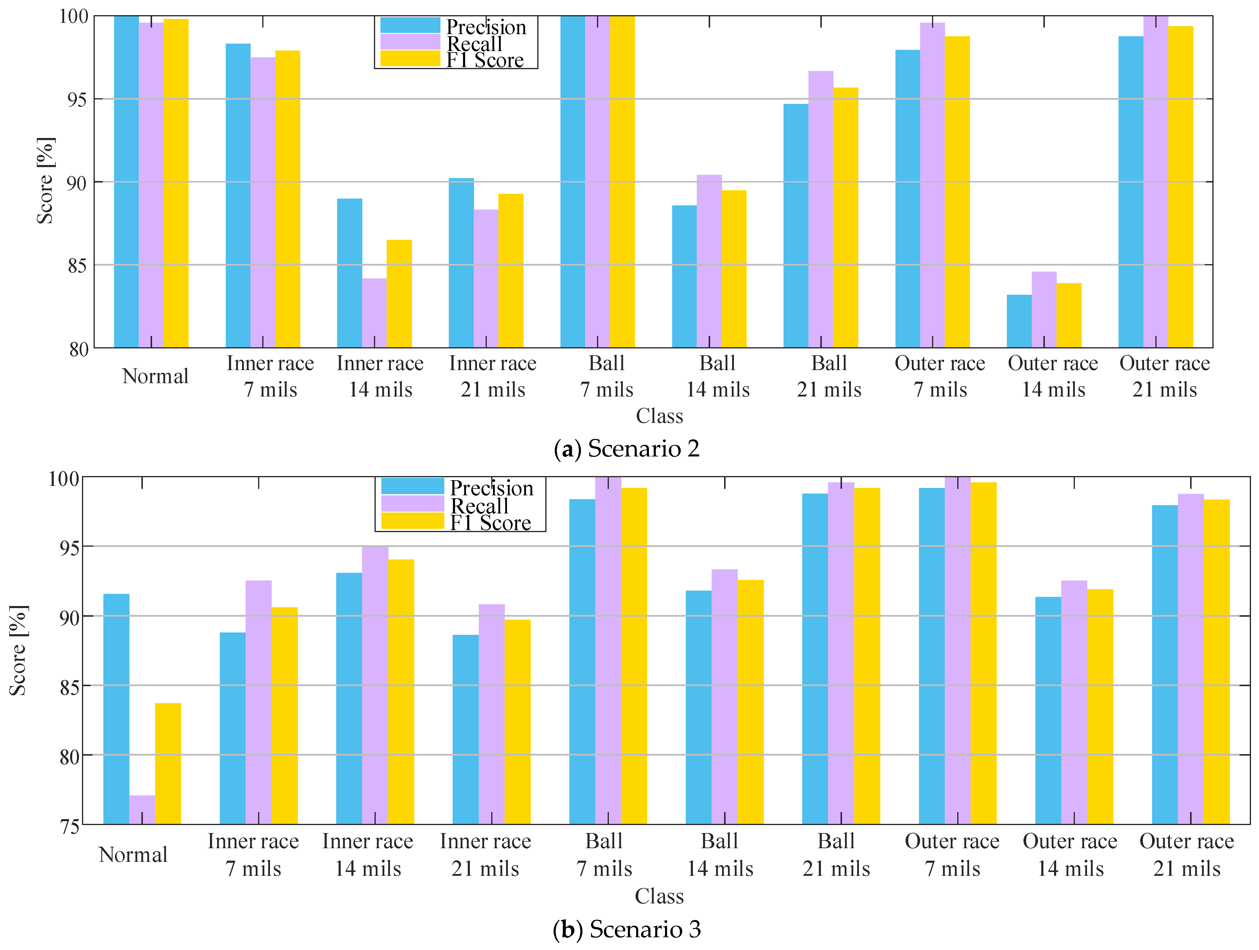
4.1. The Necessity of Sampling Frequency Unification

In current research practices, a prevalent approach involves generating training, validation, and testing sets using input data with a uniform sampling rate, a method that has demonstrated effectiveness in numerous studies. However, in the practical operation of rolling bearings, acquired signals may exhibit varying sampling rates. Due to practical constraints, it may become necessary to use data with a lower sampling rate as input for the test set with a pre-trained model, a common occurrence in engineering applications. Nevertheless, whether directly utilizing measurement data with different sampling rates as input impacts the classification accuracy of the model remains a question requiring further quantitative investigation.
To delve deeper into this issue, we designed three quantitative research scenarios outlined in Table 3. Specifically, Scenario 1 corresponds to the findings presented in Section 3 of this paper, which examines the situation where the input data under Flag 0 are upsampled from 12 kHz to 48 kHz, with its performance depicted in Table 2 and Figure 8. In Scenario 2, all other conditions are held constant, and the model is trained and evaluated using a 12 kHz sampling rate, with the performance given in Table 4 and Figure 9a. In Scenario 3, the model is trained at 48 kHz, but the input prediction data for normal conditions retain a 12 kHz sampling rate without any upsampling. The corresponding performances are shown in Table 5 and Figure 9b. Through a comparative analysis of the results, the following conclusions can be drawn:
In Scenario 2, while achieving a prediction accuracy of 94.1% using 12 kHz data for both training and prediction, the performance of the parallel DCNN model is compromised compared to its representation at higher sampling rates due to the loss of detailed vibration signal information. This finding underscores the significant influence of sampling rate selection on model performance.
In Scenario 3, when the model is trained at 48 kHz, but some input samples have a sampling rate of 12 kHz, there is a notable decrease in the model’s generalizability. Comparing the results of Case 1 and Case 3, it can be observed that when all other conditions remain unchanged and only the sampling rate of the prediction data for the bearing under normal operation is reduced to 12 kHz, the recall rate of label 0 drops significantly to approximately 77.1%. This suggests that a portion of the measurement signals during normal operation have been falsely classified as other types. Consequently, the overall accuracy of Case 3 decreases from approximately 97% to 94%, almost reaching the same level as Case 2. Nevertheless, the precision rate of label 0 remains at a high level, indicating that fault conditions of other types are rarely misclassified as normal operation, as the sampling rate for these faults remains at 48 kHz.
In conclusion, to ensure optimal training and prediction accuracy, it is imperative to standardize the sampling rate of all acquired signals before training and testing. This not only reduces the likelihood of information loss and misclassification but also enhances the model’s generalizability and overall performance.

4.2. Comparison with Existing Methods

To compare the fault diagnosis method proposed in this study with existing methods, the methodology outlined in [37] is employed. This involves the extraction of both time-domain and frequency-domain signals from operational rolling bearings. Once the necessary features are constructed, the support vector machine (SVM) is utilized to identify ten distinct states under varying load conditions. The implementation of SVM is facilitated by LIBSVM software, as described in [38]. To maintain consistency with the proposed method, the same validation approach is adopted, where data from 1 hp, 2 hp, and 3 hp load conditions are used as the training set, while data from the 0 hp condition serve as the test set. Two distinct feature construction strategies are considered:
  • Frequency-domain features: This entails the application of EEMD to decompose the vibration signals of rolling bearings into nine distinct modes. Subsequently, the first five IMFs and four residual components are extracted. Hilbert transforms are then performed on each IMF to generate five envelope spectra, each with a data length of 4800. These spectra are concatenated to form a comprehensive feature vector, which is then fed into the SVM for training and classification.
  • Time-domain features: The raw time-domain signals, with a length of 4800, are directly fed into the SVM for training and classification without any intermediate transformations or decompositions.
According to Table 6, the results indicate that when traditional SVMs are utilized in rolling bearings, the direct incorporation of pure time-domain signals as input leads to a mere 18.79% accuracy. This performance underscores the inadequacy of solely relying on these signals to accurately capture the intricate nature of the testing data. Therefore, it becomes evident that, particularly under varying load conditions, relying solely on time-domain signals is not a viable strategy for bearing fault diagnosis.
To address this limitation and fully capitalize on the distinct vibrational patterns hidden within the input time series, the EEMD technique is introduced in the comparative analysis to improve the effectiveness of the SVM. EEMD has emerged as an adaptive signal processing tool capable of decomposing intricate nonlinear and non-stationary signals into a collection of simpler IMFs. By carefully selecting the most informative IMFs and extracting their envelope spectra via Hilbert transforms, a more comprehensive and nuanced feature representation space is constructed. This meticulous approach elevates the SVM’s accuracy to 65.25%, indicating a substantial improvement. Nevertheless, despite this enhancement, a significant disparity remains when juxtaposed against the proposed method based on the GAF transform and parallel DCNN. This discrepancy underscores the inherent limitations of shallow learning algorithms and structures when confronted with high-dimensional feature data. Conversely, the proposed methodology, fortified by its robust feature extraction and learning capabilities, proves more adept at navigating the complexities inherent in such data, attaining an exceptional 97% accuracy.

5. Discussions

Modifications are made to the architecture of the established parallel DCNN to further assess the fault diagnosis capabilities of the proposed method across varying network structures. Specifically, the convolutional layers are fixed at 1, 2, and 3 while maintaining consistent conditions, as outlined in Figure 3. This entails optimizing the hyperparameters for each convolutional layer count to ensure the representation of the highest fault diagnosis accuracy achievable in each scenario.
Following the completion of model training, quantitative testing is conducted to evaluate the fault diagnosis performance of the proposed principle using a large sample size. For each network configuration, 200 sets of test samples, comprising 10,000 data points per set, are randomly extracted from the test dataset. The training and convergence processes for these scenarios are detailed in Figure 10, while the results obtained under large sample conditions are presented in Figure 11.
The findings indicate that when the number of convolutional layers is limited to 1, the convolutional neural network lacks the necessary depth to effectively extract spatial and temporal information from the GASF and GADF images resulting from polar coordinate transformation. As a result, the accuracy improvement during training is slow and remains unstable even after 1200 epochs. Additionally, the decrease in loss with increasing epochs is relatively gradual, culminating in maximum, minimum, and median test accuracies of only 87.90%, 85.88%, and 84.22%, respectively, as shown in Figure 11. In contrast, when the convolutional layers are increased to 2 or 3, the parallel DCNN demonstrates strong convergence during training, with a rapid decrease in the loss function to the order of 10−4. Under a large number of test samples, no significant differences are observed in the maximum, minimum, or median test results between these two configurations. Given their comparable performance, simpler network structures are preferred to enhance real-time capabilities.

6. Conclusions

This paper combines the strengths of both the GAF and the parallel DCNN to enhance the performance of bearing fault diagnosis. Additionally, the limitations imposed by conventional methods’ strict requirements on input data sampling rates and operating conditions are addressed. The conclusions are summarized as follows:
(1)
A method for selecting the time window of input signals is proposed based on the characteristic frequencies of vibration signals associated with different fault modes. By utilizing a 0.1-s time window, the input signals effectively capture a wide range of characteristic frequencies.
(2)
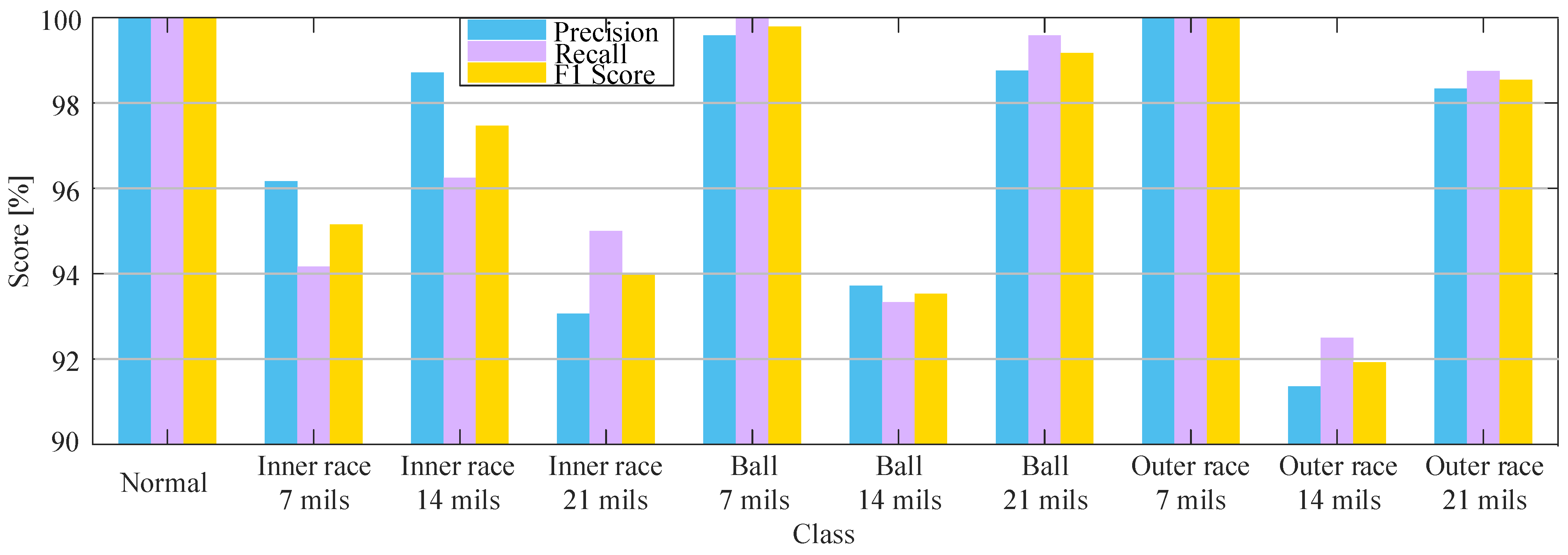
With the GAF transform, one-dimensional time series are transformed into two distinct image representations: the GASF and the GADF. These images are subsequently used as inputs for two parallel DCNN channels. An attention mechanism is employed to merge the outputs effectively. In the absence of training data within the test set, the proposed method achieves remarkable performance, with accuracy rates ranging from 91.36% to 100%, recall rates between 92.50% and 100%, and F1 scores varying from 91.93% to 100%. Overall, the method achieves a remarkable 96.96% improvement.
(3)
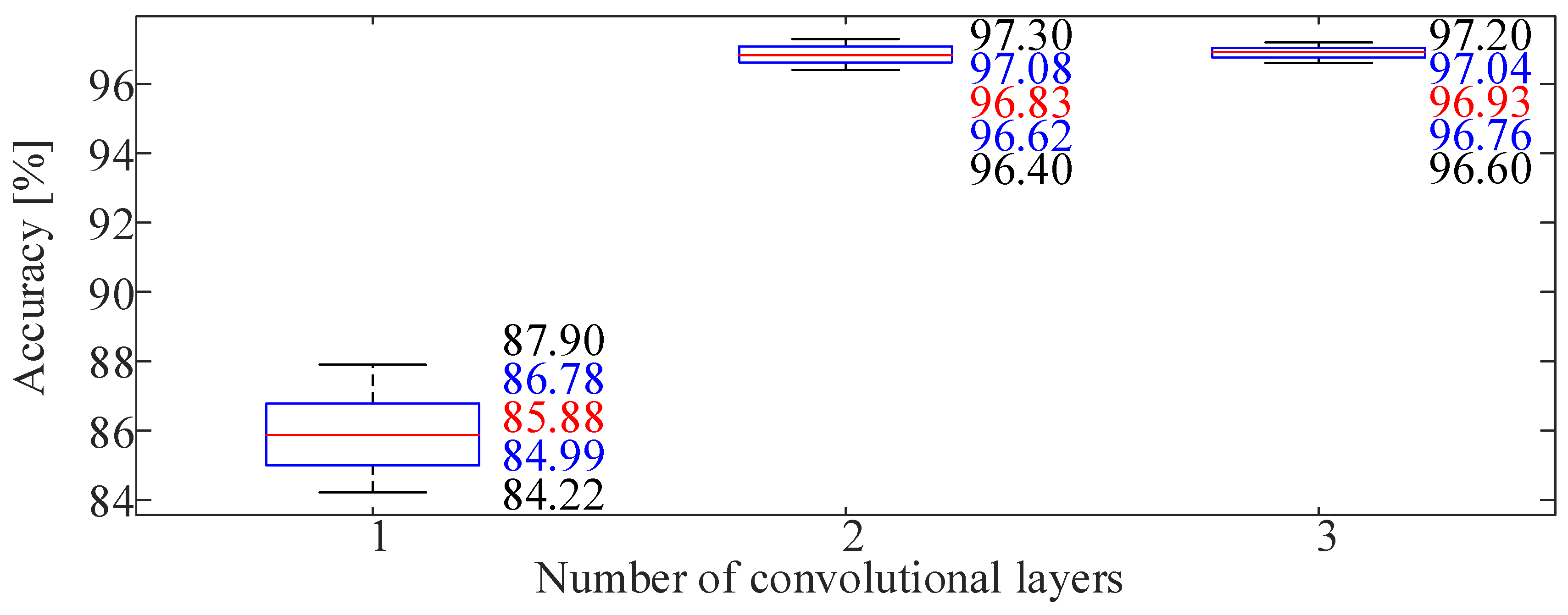
This paper further investigates the impact of different network structures on key performance metrics. The results reveal that using two convolutional layers are sufficient to provide robust fault diagnosis capabilities. Specifically, in scenarios involving large sample sizes and repetitive trials, the median accuracy reaches 96.83%, significantly surpassing the 85.88% achieved with one convolutional layer. Further, increasing the number of convolutional layers does not result in additional improvements.
(4)
The necessity of unifying the sampling rate is examined using the control variable method. Feeding time series data obtained at different sampling rates into a trained model can decrease the fault identification accuracy to approximately 94%. Such degradation can be partly solved according to this study. Challenges remain when the model’s sampling rate is not an integer multiple of the input data’s rate.

Author Contributions

Conceptualization, Z.L. and N.T.; methodology, Z.L. and Y.W.; software, Z.L. and Y.W.; validation, Z.L. and N.T.; formal analysis, Y.G. and F.W.; investigation, Y.G. and F.W.; resources, F.W. and N.T.; data curation, X.T. and F.W.; writing—original draft preparation, Z.L.; writing—review and editing, Z.L.; visualization, Z.L.; supervision, Y.W.; project administration, N.T.; funding acquisition, N.T. All authors have read and agreed to the published version of the manuscript.

Funding

This research was funded by the Natural Science Foundation of Guangdong Province under Grants 2024A1515012720 and 2023A1515240082.

Data Availability Statement

Data supporting this study cannot be made available because the research data are confidential. This is because of the arrangement the research groups have made with the commercial partner supporting the research.

Conflicts of Interest

The authors declare no conflicts of interest.

References

  1. Wang, S.; Chen, X.; Tong, C.; Zhao, Z. Matching synchrosqueezing wavelet transform and application to aeroengine vibration monitoring. IEEE Trans. Instrum. Meas. 2016, 66, 360–372. [Google Scholar] [CrossRef]
  2. Wang, S.; Chen, X.; Selesnick, I.W.; Guo, Y.; Tong, C.; Zhang, X. Matching synchrosqueezing transform: A useful tool for characterizing signals with fast varying instantaneous frequency and application to machine fault diagnosis. Mech. Syst. Signal Proc. 2018, 100, 242–288. [Google Scholar] [CrossRef]
  3. Yu, G.; Lin, T.R. Second-order transient-extracting transform for the analysis of impulsive-like signals. Mech. Syst. Signal Proc. 2021, 147, 107069. [Google Scholar] [CrossRef]
  4. Geetha, G.; Geethanjali, P. An efficient method for bearing fault diagnosis. Syst. Sci. Control Eng. 2024, 12, 2329264. [Google Scholar] [CrossRef]
  5. Wu, Z.; Huang, N.E. Ensemble empirical mode decomposition: A noise-assisted data analysis method. Adv. Adapt. Data Anal. 2009, 1, 1–41. [Google Scholar] [CrossRef]
  6. Roy, A.; Doherty, J.F. Raised cosine filter-based empirical mode decomposition. IET Signal Process. 2011, 5, 121–129. [Google Scholar] [CrossRef]
  7. Soman, A.; Sarath, R. Optimization-enabled deep convolutional neural network with multiple features for cardiac arrhythmia classification using ECG signals. Biomed. Signal Process. Control 2024, 92, 105964. [Google Scholar] [CrossRef]
  8. Del E Chelle, E.; Lemoine, J.; Niang, O. Empirical mode decomposition: An analytical approach for sifting process. IEEE Signal Process. Lett. 2005, 12, 764–767. [Google Scholar] [CrossRef]
  9. Myat, A.; Kondath, N.; Soh, Y.L.; Hui, A. A hybrid model based on multivariate fast iterative filtering and long short-term memory for ultra-short-term cooling load prediction. Energy Build. 2024, 307, 113977. [Google Scholar] [CrossRef]
  10. Cicone, A.; Liu, J.; Zhou, H. Adaptive local iterative filtering for signal decomposition and instantaneous frequency analysis. Appl. Comput. Harmon. Anal. 2016, 41, 384–411. [Google Scholar] [CrossRef]
  11. Guo, B.; Peng, S.; Hu, X.; Xu, P. Complex-valued differential operator-based method for multi-component signal separation. Signal Process. 2017, 132, 66–76. [Google Scholar] [CrossRef]
  12. Dubey, R.; Sharma, R.R.; Upadhyay, A.; Pachori, R.B. Automated Variational Nonlinear Chirp Mode Decomposition for Bearing Fault Diagnosis. IEEE Trans. Ind. Inform. 2023, 19, 10873–10882. [Google Scholar] [CrossRef]
  13. Chen, S.; Yang, Y.; Peng, Z.; Dong, X.; Zhang, W.; Meng, G. Adaptive chirp mode pursuit: Algorithm and applications. Mech. Syst. Signal Proc. 2019, 116, 566–584. [Google Scholar] [CrossRef]
  14. Chen, S.; Dong, X.; Xing, G.; Peng, Z.; Zhang, W.; Meng, G. Separation of overlapped non-stationary signals by ridge path regrouping and intrinsic chirp component decomposition. IEEE Sens. J. 2017, 17, 5994–6005. [Google Scholar] [CrossRef]
  15. Dong, X.; Chen, S.; Xing, G.; Peng, Z.; Zhang, W.; Meng, G. Doppler frequency estimation by parameterized time-frequency transform and phase compensation technique. IEEE Sens. J. 2018, 18, 3734–3744. [Google Scholar] [CrossRef]
  16. Guo, W.; Jiang, X.; Li, N.; Shi, J.; Zhu, Z. A coarse TF ridge-guided multi-band feature extraction method for bearing fault diagnosis under varying speed conditions. IEEE Access 2019, 7, 18293–18310. [Google Scholar] [CrossRef]
  17. Tamilselvan, P.; Wang, P. Failure diagnosis using deep belief learning based health state classification. Reliab. Eng. Syst. Saf. 2013, 115, 124–135. [Google Scholar] [CrossRef]
  18. Yang, Y.; Peng, Z.K.; Dong, X.J.; Zhang, W.M.; Meng, G. General parameterized time-frequency transform. IEEE Trans. Signal Process. 2014, 62, 2751–2764. [Google Scholar] [CrossRef]
  19. Li, X.; Bi, G.; Stankovic, S.; Zoubir, A.M. Local polynomial Fourier transform: A review on recent developments and applications. Signal Process. 2011, 91, 1370–1393. [Google Scholar] [CrossRef]
  20. Peng, Z.K.; Meng, G.; Chu, F.L.; Lang, Z.; Zhang, W.M.; Yang, Y. Polynomial chirplet transform with application to instantaneous frequency estimation. IEEE Trans. Instrum. Meas. 2011, 60, 3222–3229. [Google Scholar] [CrossRef]
  21. Yu, G. A concentrated time--frequency analysis tool for bearing fault diagnosis. IEEE Trans. Instrum. Meas. 2019, 69, 371–381. [Google Scholar] [CrossRef]
  22. Yu, G.; Wang, Z.; Zhao, P.; Li, Z. Local maximum synchrosqueezing transform: An energy-concentrated time-frequency analysis tool. Mech. Syst. Signal Proc. 2019, 117, 537–552. [Google Scholar] [CrossRef]
  23. Xu, G.; Liu, M.; Jiang, Z.; S O Ffker, D.; Shen, W. Bearing fault diagnosis method based on deep convolutional neural network and random forest ensemble learning. Sensors 2019, 19, 1088. [Google Scholar] [CrossRef] [PubMed]
  24. Guo, X.; Chen, L.; Shen, C. Hierarchical adaptive deep convolution neural network and its application to bearing fault diagnosis. Measurement 2016, 93, 490–502. [Google Scholar] [CrossRef]
  25. Zhang, W.; Peng, G.; Li, C.; Chen, Y.; Zhang, Z. A new deep learning model for fault diagnosis with good anti-noise and domain adaptation ability on raw vibration signals. Sensors 2017, 17, 425. [Google Scholar] [CrossRef]
  26. Hoang, D.; Kang, H. A survey on deep learning based bearing fault diagnosis. Neurocomputing 2019, 335, 327–335. [Google Scholar] [CrossRef]
  27. Li, X.; Zhang, W.; Ding, Q.; Sun, J. Intelligent rotating machinery fault diagnosis based on deep learning using data augmentation. J. Intell. Manuf. 2020, 31, 433–452. [Google Scholar] [CrossRef]
  28. Biswas, S.; Panigrahi, B.K.; Nayak, P.K.; Pradhan, G.; Padmanaban, S. A Single-Pole Filter Assisted Improved Protection Scheme for the TCSC Compensated Transmission Line Connecting Large-Scale Wind Farms. IEEE J. Emerg. Sel. Top. Ind. Electron. 2023, 1–13. [Google Scholar] [CrossRef]
  29. Biswas, S.; Nayak, P.K.; Panigrahi, B.K.; Pradhan, G. An intelligent fault detection and classification technique based on variational mode decomposition-CNN for transmission lines installed with UPFC and wind farm. Electr. Power Syst. Res. 2023, 223, 109526. [Google Scholar] [CrossRef]
  30. Romano, D.; Kovacevic-Badstuebner, I.; Antonini, G.; Grossner, U. Accelerated Evaluation of Quasi-Static Interaction Integrals via Cubic Spline Interpolation in the Framework of the PEEC Method. IEEE Trans. Electromagn. Compat. 2024, 1–8. [Google Scholar] [CrossRef]
  31. Li, S.; Jia, J. A Cost-Efficient Numerical Algorithm for Evaluating the Determinant of a Quasi-Tridiagonal Matrix. In Proceedings of the 2018 5th International Conference on Systems and Informatics (ICSAI), Nanjing, China, 10–12 November 2018; IEEE: Piscataway, NJ, USA, 2018; pp. 593–597. [Google Scholar]
  32. Wang, Z.; Oates, T. Imaging time-series to improve classification and imputation. arXiv 2015, arXiv:1506.00327. [Google Scholar]
  33. Wu, D.; Wang, J.; Wang, H.; Liu, H.; Lai, L.; He, T.; Xie, T. An automatic bearing fault diagnosis method based on characteristics frequency ratio. Sensors 2020, 20, 1519. [Google Scholar] [CrossRef]
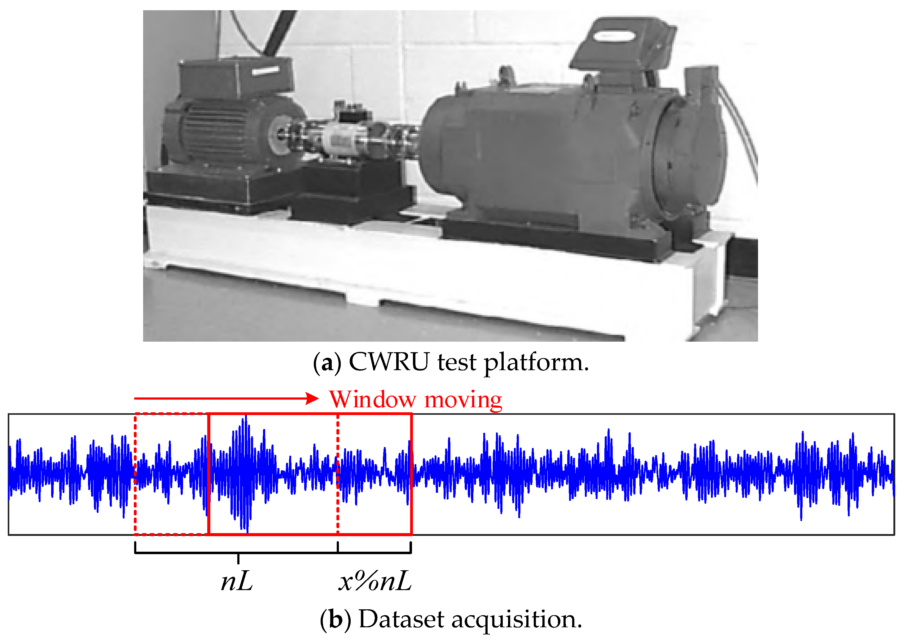
  34. Neupane, D.; Seok, J. Bearing fault detection and diagnosis using case western reserve university dataset with deep learning approaches: A review. IEEE Access 2020, 8, 93155–93178. [Google Scholar] [CrossRef]
  35. Case Western Reserve University Bearing Data Center. Available online: https://csegroups.case.edu/bearingdatacenter/home (accessed on 22 December 2019).
  36. Thévenaz, P. Image Interpolation and Resampling. In Handbook of Medical Imaging; Academic Press: San Diego, CA, USA, 2000. [Google Scholar]
  37. Kang, S.; Ma, D.; Wang, Y.; Lan, C.; Chen, Q.; Mikulovich, V.I. Method of assessing the state of a rolling bearing based on the relative compensation distance of multiple-domain features and locally linear embedding. Mech. Syst. Signal Proc. 2017, 86, 40–57. [Google Scholar] [CrossRef]
  38. Chang, C.; Lin, C. LIBSVM: A library for support vector machines. ACM Trans. Intell. Syst. Technol. 2011, 2, 21–27. [Google Scholar] [CrossRef]
Figure 1. Four types of defects for rolling bearings.
Symmetry 16 00432 g001
Figure 2. The structure of the constructed parallel DCNN.
Symmetry 16 00432 g002
Figure 4. The CWRU test platform for machinery faults.
Symmetry 16 00432 g004
Figure 5. Sampling frequency unification.
Symmetry 16 00432 g005
Figure 6. An example of a GAF transform.
Symmetry 16 00432 g006
Figure 7. Comparison among different training datasets.
Symmetry 16 00432 g007
Figure 8. Performance of the proposed method.
Symmetry 16 00432 g008
Figure 9. Indicator comparison.
Symmetry 16 00432 g009
Figure 10. Comparison among different DCNN structures.
Symmetry 16 00432 g010
Figure 11. Large-scale test case results. Note *: The box plot presents the upper edge, upper quartile, median, lower quartile, and lower edge, distinguished by various colors. The adjacent numerals precisely correspond to the positions and dispersions of the respective data points within the box plot.
Symmetry 16 00432 g011
Table 1. Categories of bearing operating conditions.
Flag0123456789
Fault
element
N.A.Inner
race
Inner
race
Inner
race
BallBallBallOuter
race
Outer
race
Outer
race
Fault
level [mils]
N.A.714217142171421
Table 2. Confusion matrix of the training data.
Test Flag0123456789
Real Flag
0240000000000
10226030000110
2002311030041
3000228083010
4000024000000
5002512240053
6000100239000
7000000024000
8091701002220
9000003000237
Table 3. Testing dataset under different sampling frequencies.
Flag0123456789
Fault
element
N.A.Inner
race
Inner
race
Inner
race
BallBallBallOuter
race
Outer
race
Outer
race
Fault
level [mils]
N.A.714217142171421
Scenario 1Number of240240240240240240240240240240
Training sampling frequency = 48 kHzSamples(48 kHz)(48 kHz)(48 kHz)(48 kHz)(48 kHz)(48 kHz)(48 kHz)(48 kHz)(48 kHz)(48 kHz)
Scenario 2Number of240240240240240240240240240240
Training sampling frequency = 12 kHzSamples(12 kHz)(12 kHz)(12 kHz)(12 kHz)(12 kHz)(12 kHz)(12 kHz)(12 kHz)(12 kHz)(12 kHz)
Scenario 3Number of240240240240240240240240240240
Training sampling frequency = 48 kHzSamples(12 kHz)(48 kHz)(48 kHz)(48 kHz)(48 kHz)(48 kHz)(48 kHz)(48 kHz)(48 kHz)(48 kHz)
The presence of “N.A.” signifies that the bearing is functioning within its normal operational range, thus indicating the absence of both fault element and fault level.
Table 4. Confusion matrix for Case 2.
Test Flag0123456789
Real Flag
0239100000000
1023401040010
201202001300231
30032120471130
4000024000000
50014402171031
6002103232011
7000100023900
80261604542030
9000000000240
Table 5. Confusion matrix for Case 3.
Test Flag0123456789
Real Flag
0185191411350201
14222030000110
2302281030041
31000218083010
4000024000000
5002512240053
6000100239000
7000000024000
8091701002220
9000003000237
Table 6. Confusion matrix of the SVM-based method.
Test Flag0123456789
Real Flag
Method
0(1)240000000000
(2)240000000000
1(1)024000000000
(2)1845600000000
2(1)13731435110040
(2)2201550000000
3(1)0156078003030
(2)1687000010640
4(1)0000167000073
(2)15465401700000
5(1)023102000610
(2)2052900060000
6(1)0004830188001
(2)2012550004005
7(1)000000024000
(2)4835110001654076
8(1)0183000000570
(2)1830000000570
9(1)0000270000213
(2)117773400000012
Disclaimer/Publisher’s Note: The statements, opinions and data contained in all publications are solely those of the individual author(s) and contributor(s) and not of MDPI and/or the editor(s). MDPI and/or the editor(s) disclaim responsibility for any injury to people or property resulting from any ideas, methods, instructions or products referred to in the content.

