1. Introduction
There has been an increased focus on blood microflow research [
1]. There are some related interesting biomedical papers researching control of microflows [
2] and drug absorption [
3,
4]. Technical advances [
5,
6,
7,
8] have made possible accurate measurements at small scale [
9,
10,
11]. Milieva et al. [
12] analyzed skin blood microflows using laser Doppler flowmetry (LDF) and compared healthy control cases to individuals with rheumatic diseases [
13]. This LDF approach has been followed in some other interesting articles, such as Zherebtsov et al. [
14]. In Zherebtsov et al., the authors used a combination of LDF with skin contact thermometry applied for the diagnostics of intradermal finger vessels. There is some research linking microflow (particularly microflow changes) and some illnesses. Wang et al. [
15] mentioned that there appears to be an association between some type of microflows in the hepatic sinusoids and liver fibrosis and cirrhosis [
16]. Microflow cytometry has been extensively used in medical applications, such as Lewis et al. [
17] for the detection of prostate cancer [
18]. There is even some research on blood microflow in the context of microchips. Pitts et al. [
19] studied the contact angle of blood dilutions with common microchip materials.
Microflow measurement techniques have substantially advanced in recent years when compared to some of the first attempts, such as Stosseck et al. [
20] in 1974. In this paper the authors measured blood microflows using electrochemically generated hydrogen. This technique requires 15 s per measurement. Another seminal paper is the one by Leniger-Follert [
21] back in 1984, which analyzed microflows during bicuculline-induced seizures [
22,
23,
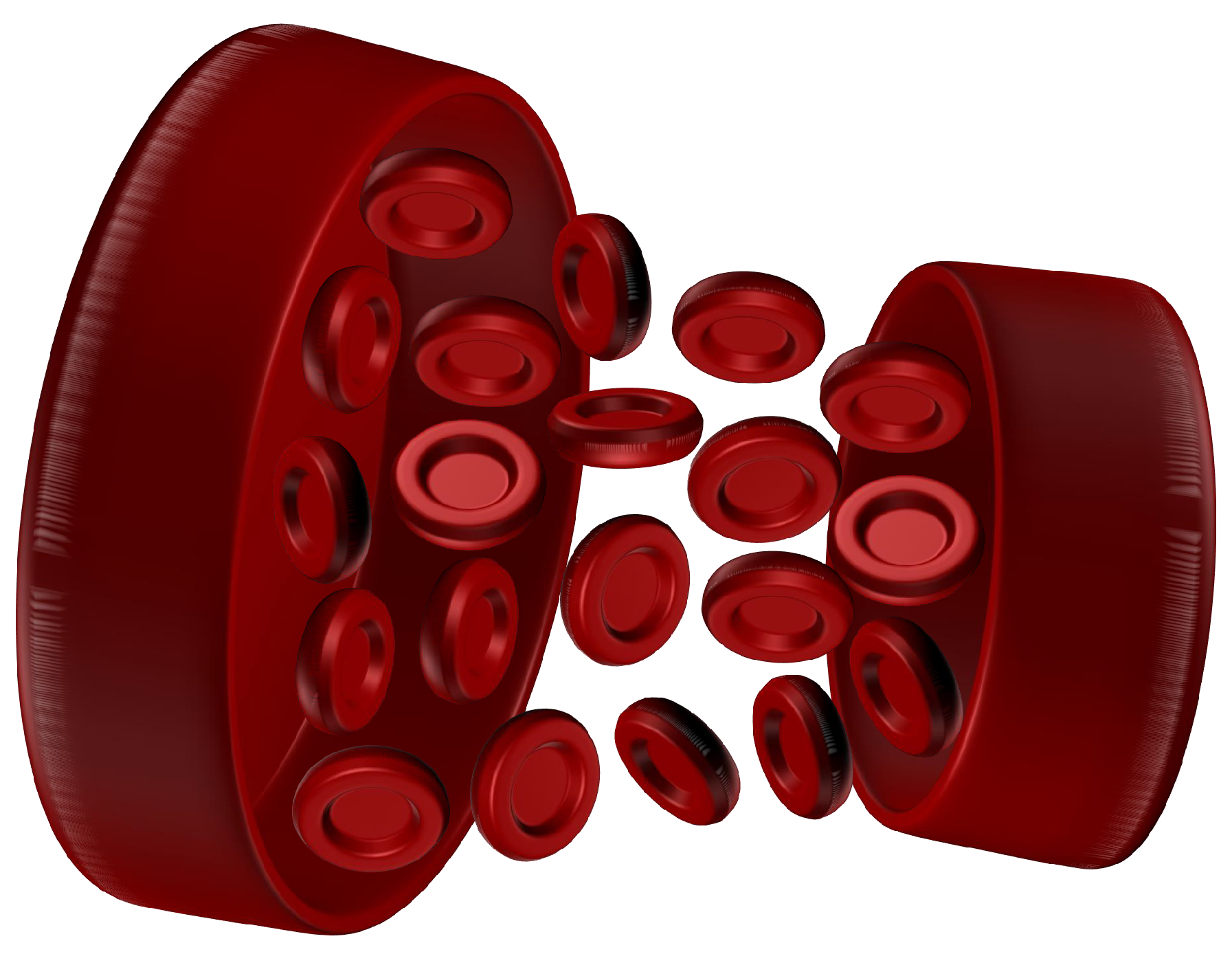
24] in anesthetized cats. In recent years, technical developments have made the measurement task more accurate and less cumbersome. In the figure below (
Figure 1), a graphical representation of red blood cell flow as a blood vessel constricts is shown.
There are some very interesting modeling articles, such as Meongkeun et al. [
25]. In this article, the authors numerically analyzed the impact of cell deformability (red blood cells) in blood microflow dynamics and concluded that the radial dispersion of red blood cells can have a significant impact on microflows. Mojarab and Kamali [
26] carried out another interesting modeling work doing a numerical simulation of a microflow sensor in a realistic model of a human aorta. This type of analysis has particular relevance in the context of artherosclerosis and aneurysm, which are conditions associated with an elevated mortality rate [
27,
28,
29]. Having a more complete understanding of blood microflows might help with understanding these conditions better and potentially help with finding ways to avoid or treat them. In fact, there is some research, such as Jung et al. [
30], mentioning that there is a correlation between microflow changes in cardiogenic shock (CS) [
31,
32,
33] and outcomes in critically ill patients.
Given the complexity of the modeling of blood microflows, there has been an increased interest in using artificial intelligence techniques to estimate some important properties of blood microflows, such as the velocity of the blood flow. These artificial intelligence techniques typically require a set of inputs, which are reasonably related to an output. If everything else is equal, the more the inputs are related to the output, the more accurate the predictions are likely to be. Understanding the underlying issue might allow researchers to select the appropriate variables as inputs for the forecasting process. Some machine learning approaches intrinsically use some of the symmetries in the existing data. One well-known artificial intelligence technique is an artificial neural network (ANN) [
34,
35,
36,
37].
This is a biologically inspired approach that has proven useful when modeling several different types of processes [
38,
39]. Paproski et al. [
40] used a machine learning approach in the context of extracellular vesicle microscale flow cytometry to generate predictive models in different types of tumors. Selecting which type of ANN architecture [
41] to use is important in order to obtain accurate forecasts. Some of the parameters to be selected include the number of neurons (
n), the number of layers (
m) and the type of training algorithm used (
a). There are several ways to select these parameters. In this article, we propose an ANN model to estimate blood microflow velocities using a grid approach [
42,
43]. It should be mentioned that the use of artificial intelligence techniques is not without a variety of issues [
44,
45,
46]. Lugnan et al. [
47] mentioned that one issue is the high computational cost of some of these applications, as discussed also in [
48,
49,
50]. An artificial intelligence approach can be useful in practical applications to generate accurate forecasts [
51,
52,
53]. The main objective of this type of model is not to develop an underlying model of microflows that is easy to interpret, but to develop a tool that can generate accurate forecasts.
1.1. Objective 1
Creation of ANN model to estimate blood microflow velocities.
1.2. Objective 2
Estimate robustness of ANN with respect to noise in inputs.
2. Materials and Methods
The data analyzed in this article were extracted from Kloosterman et al. [
54] (publicly available data). As described in Kloosterman et al., fertilized chicken (White Leghorn) embryos were incubated sitting horizontally. The authors generated optical access to the embryos by creating a viewing window in the egg shell. This window provided a microscope with optical access to the embryos. The technique used by the authors for the measurements was microscopic particle image velocimetry (micro-PIV). The authors used a Leica FluoCombi III with a magnification of 5×. They also used a PCO Sensicam QE camera with a pixel size of 12.9 × 12.9
m
2 and covering an area of 1.8 × 1.4 mm
2 (full details available in [
54]). We use the data from Kloosterman et al. as the experimental data on which our analysis is based.
Our proposed approach generates estimates of the velocity of the blood in a chicken embryo, which will be compared to the empirical results obtained in Kloosterman et al. This approach uses as input the positions (coordinates of the branch points
) as well as the diameter
of the blood vessel, which ranges from 25 to 500
m, as well as the velocity
in the blood vessels in the previous instant. The sampling rate for
was 9.7 Hz. The velocity was normalized to the interval [0, 1] using the expression in Equation (
1). The velocity was also smoothed by using the average value of the previous ten measurements. After the initial filtering (including normalization), the data consisted of 379 data points for each variable. A table summarizing the descriptive statistics for each variable can be seen as
Table 1.
An artificial neural network only requires a set of inputs and an output y. These inputs and outputs are typically vectors. So and , with the last time instant k included. The selection of which inputs to use is a critical step in the modeling process, but this might be restricted by the availability of the data. The objective of the model is to accurately estimate the empirically measured blood microflow velocity .
In this notation, t denotes time. The data were divided into two different datasets: a testing
and a training
dataset. See Equations (
2) and (
3).
where
j and
q are predetermined parameters dividing the training and testing datasets. The dataset contained 379 data points per variable; 85% of the data were allocated to the training dataset, and 15% were allocated to the testing dataset. The training dataset was further divided into the strictly training subset (65%) and the validation subset (20%). The neural network was trained with the training dataset
.
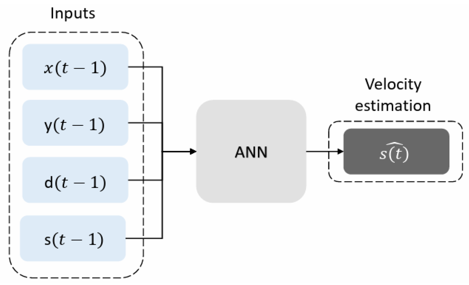
For clarity purposes, we have added an example of the inputs and outputs of the neural network, see
Table 2, and a graphical representation in
Figure 2.
2.1. Data Mappings
It is important to have a sense of the mapping of the inputs and outputs. In this section, we analyze the mapping of each input (
,
,
) with the output (
). Hence, we can consider four mappings as shown in
Table 3.
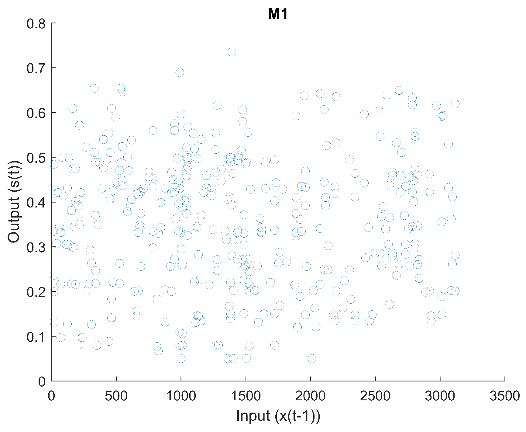
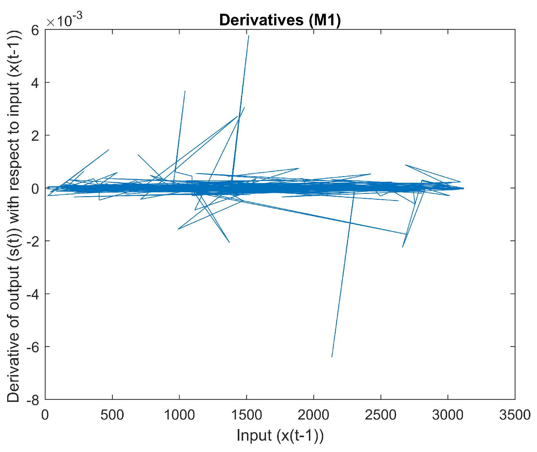
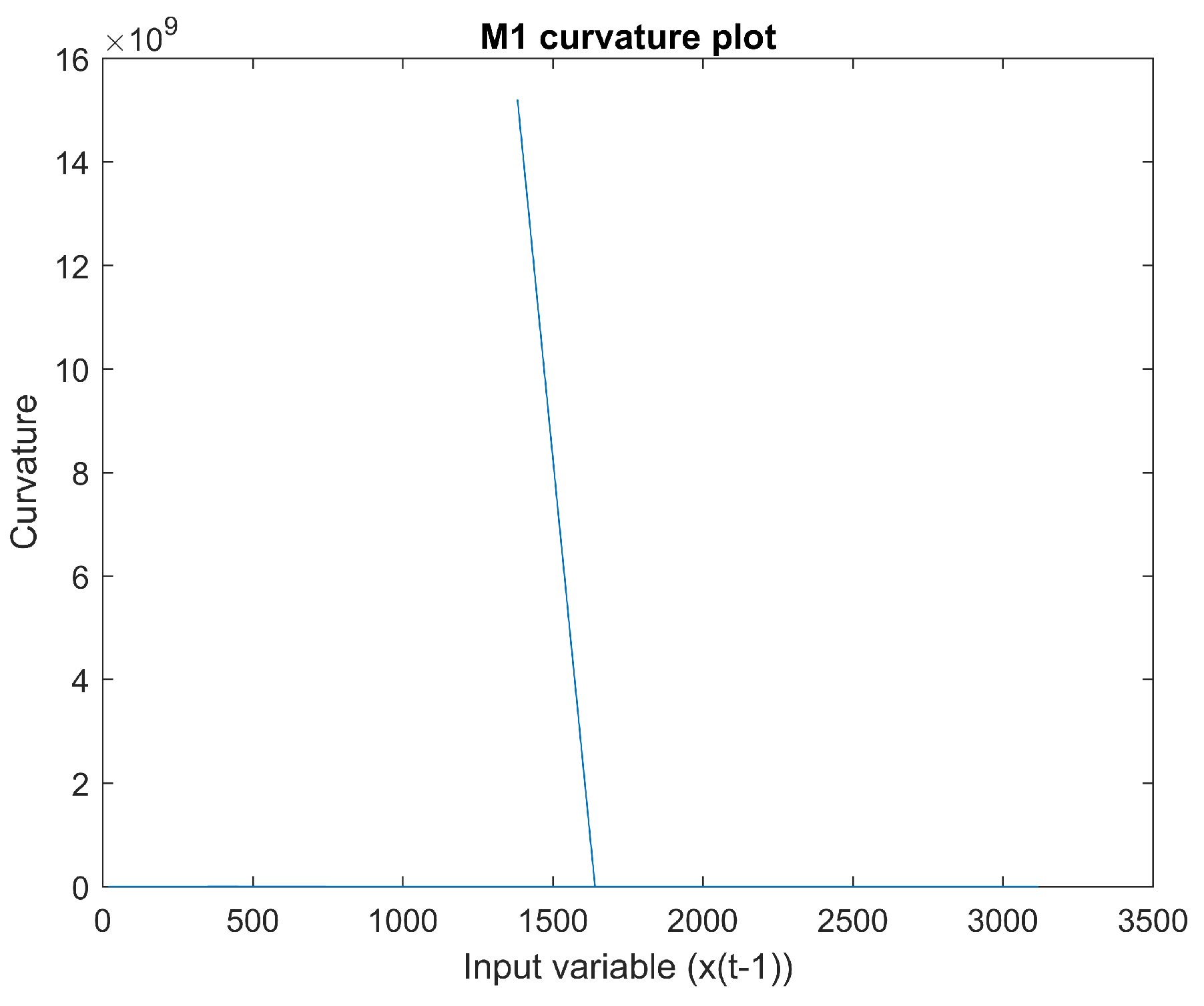
2.1.1. Mapping 1
Figure 3 is a scatter plot of input
vs. output
. The derivative of input
with regard to output
can be seen in
Figure 4. There appear to be sudden changes in the derivative. The curvature of a mapping of an input “in” and an output “o” can be estimated using Equation (
4), where
is the arch of the length of the analyzed curve. In this notation,
is the fist derivative, and
is the second derivative. Also, as an example, the input for M1 is
, and the output is
. This is done for each mapping shown in
Table 3. The curvature of this mapping can be seen in
Figure 5. The curvature does not appear to be smooth.
A lineal model, as described in Equation (
5), is another technique to analyze this mapping. The obtained adjusted
in this model is −0.002522; see
Table 4.
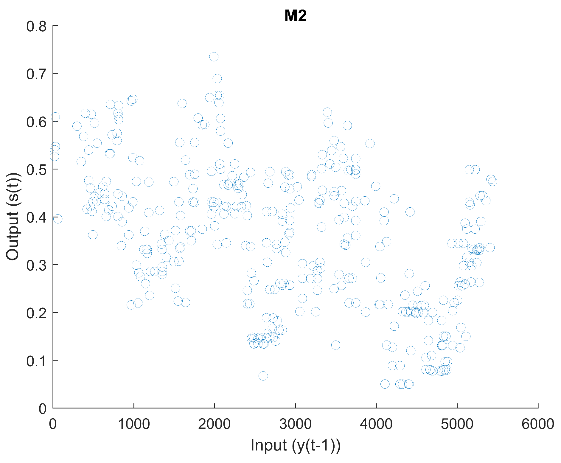
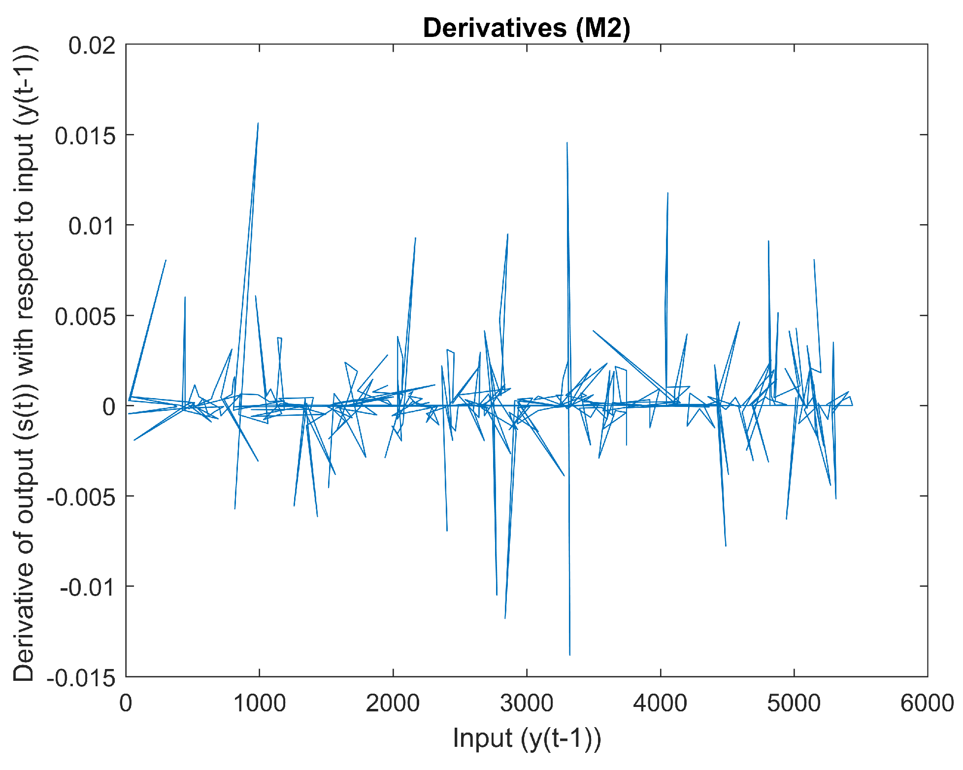
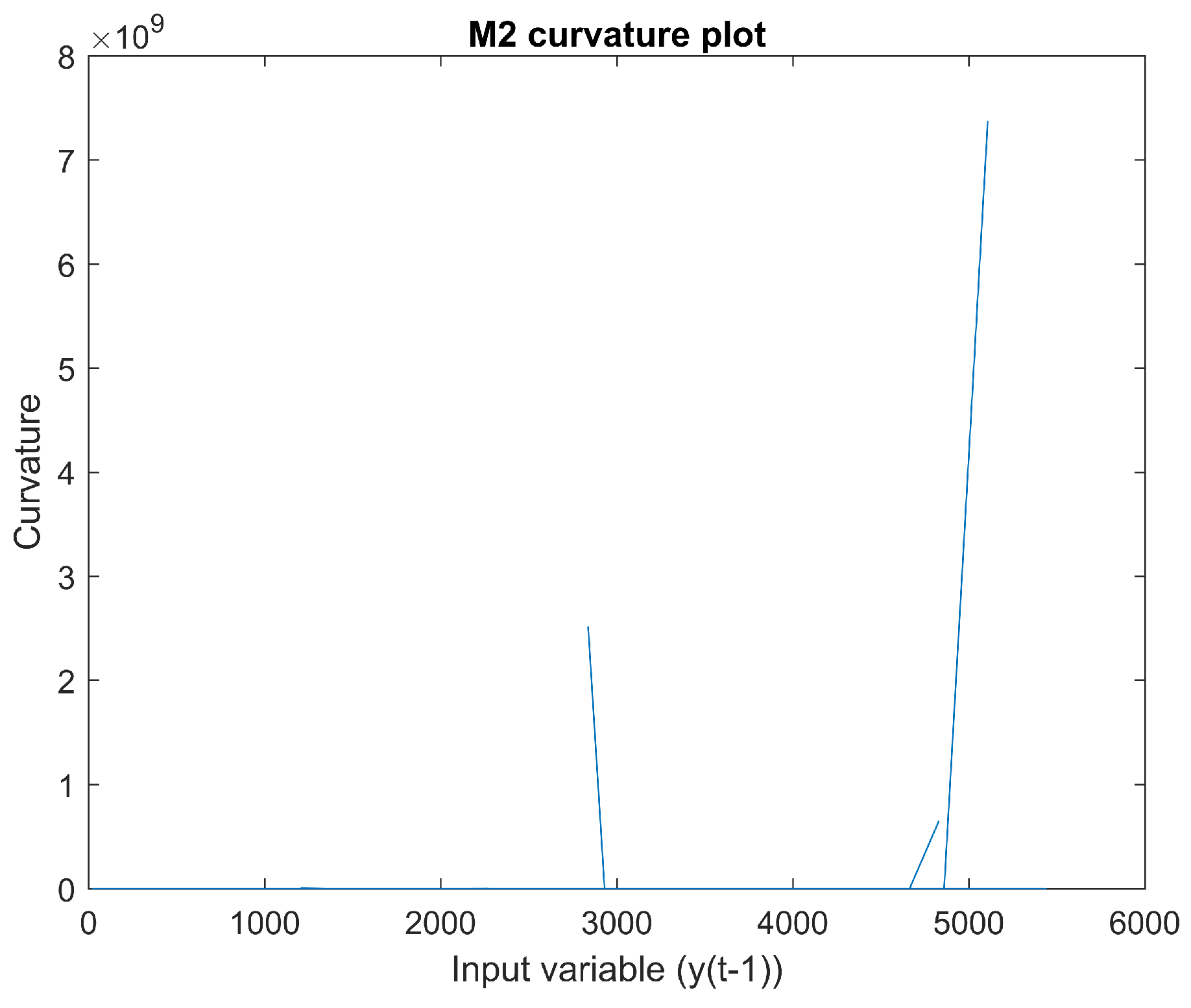
2.1.2. Mapping 2
Figure 6 is a scatter plot of input
vs. output
. The derivative of input
with regard to output
can be seen in
Figure 7. There appear to be sudden changes in the derivative. The curvature of this mapping can be seen in
Figure 8. The curvature does not appear to be smooth.
A lineal model, as described in Equation (
6), is another technique to analyze this mapping. The obtained adjusted
in this model is 0.2277; see
Table 5. Please notice that this time series, as will shown in the next section, is not stationary. Hence, a direct implementation of a linear model is not appropriate.
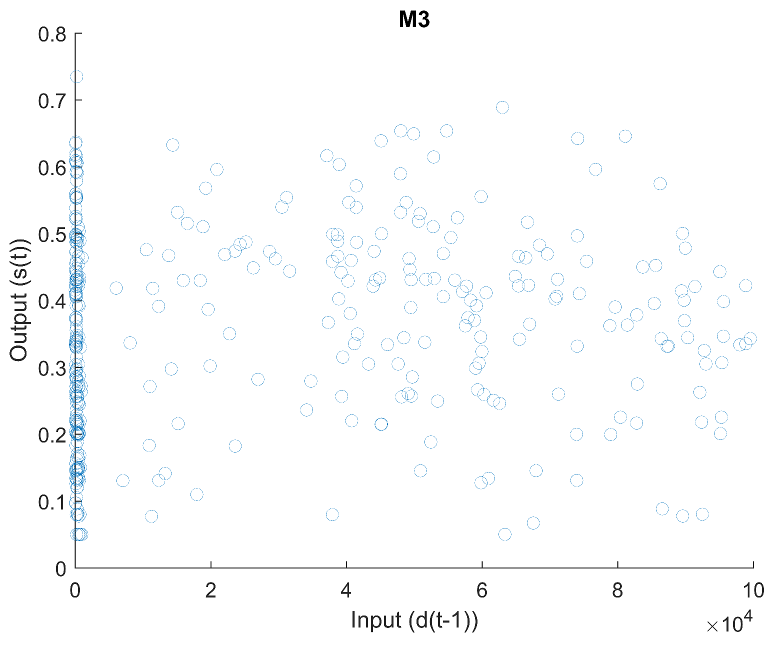
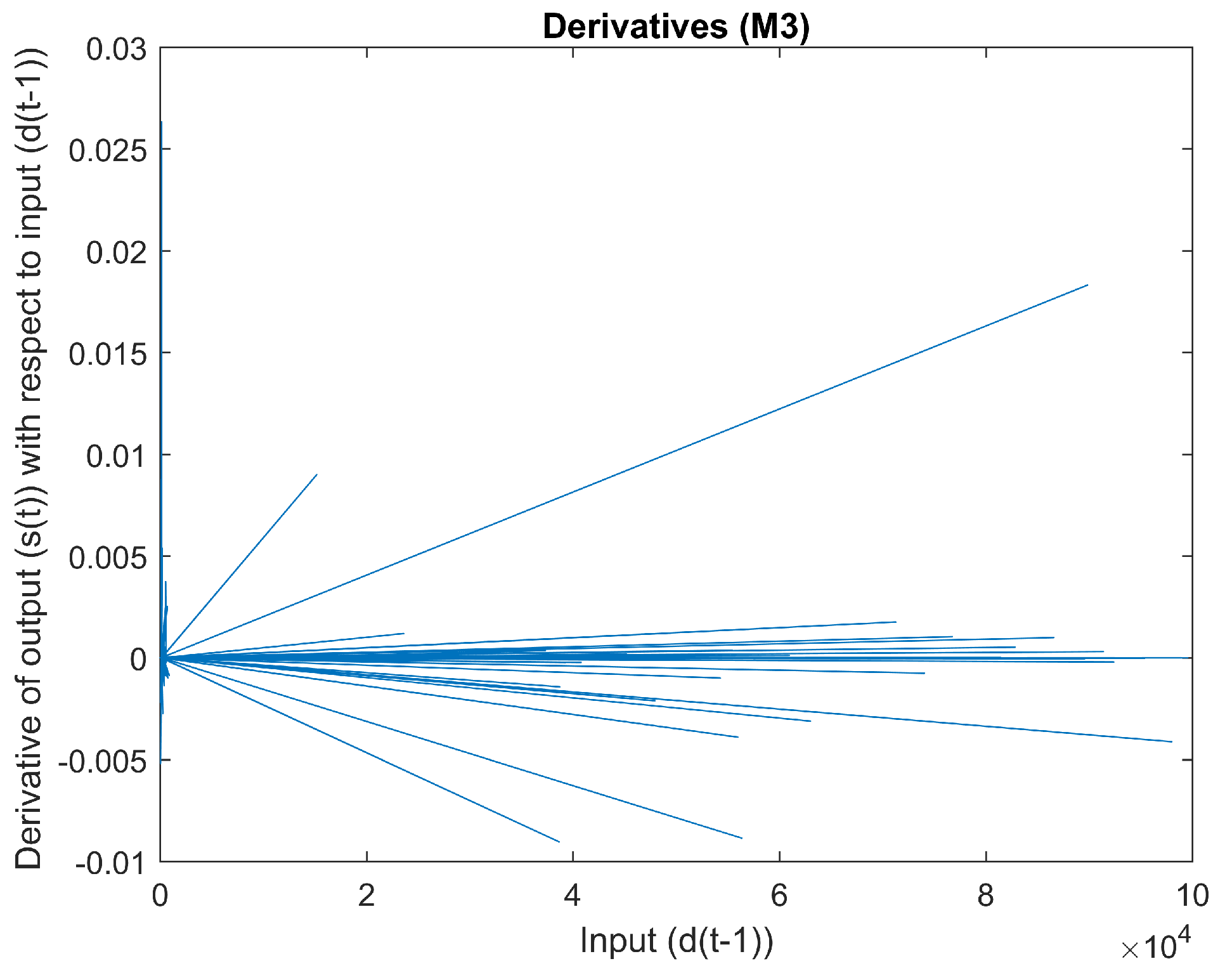
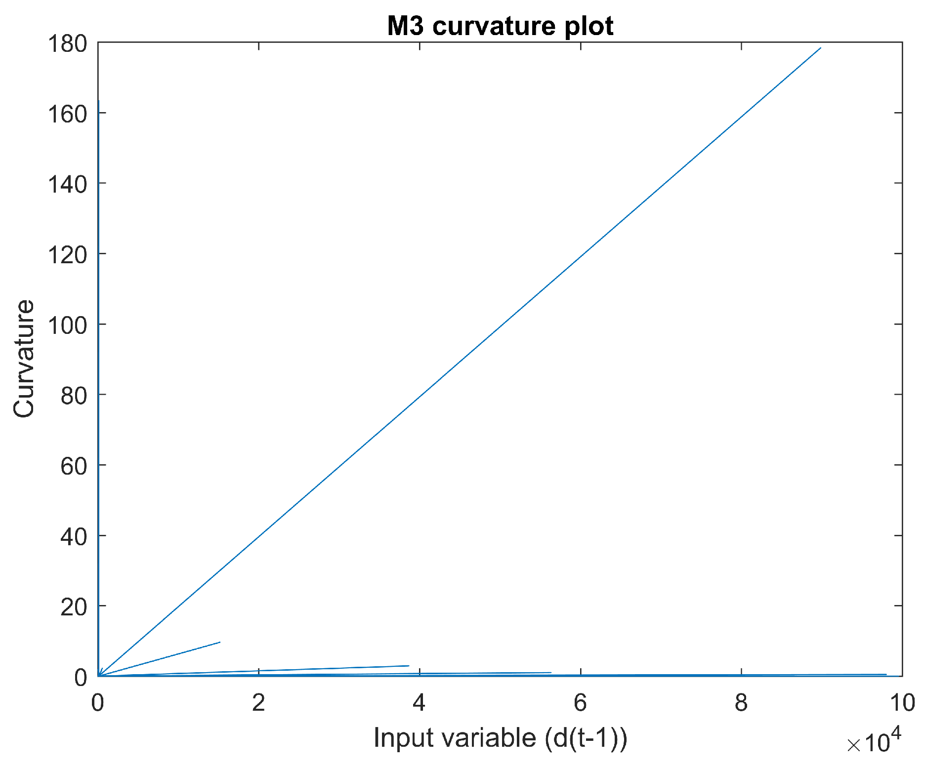
2.1.3. Mapping 3
Figure 9 is a scatter plot of input
vs. output
. The derivative of input
with regard to output
can be seen in
Figure 10. There appear to be sudden changes in the derivative. The curvature of this mapping can be seen in
Figure 11. The curvature does not appear to be smooth.
A lineal model, as described in Equation (
7), is another technique to analyze this mapping. The obtained adjusted
in this model is 0.01819; see
Table 6.
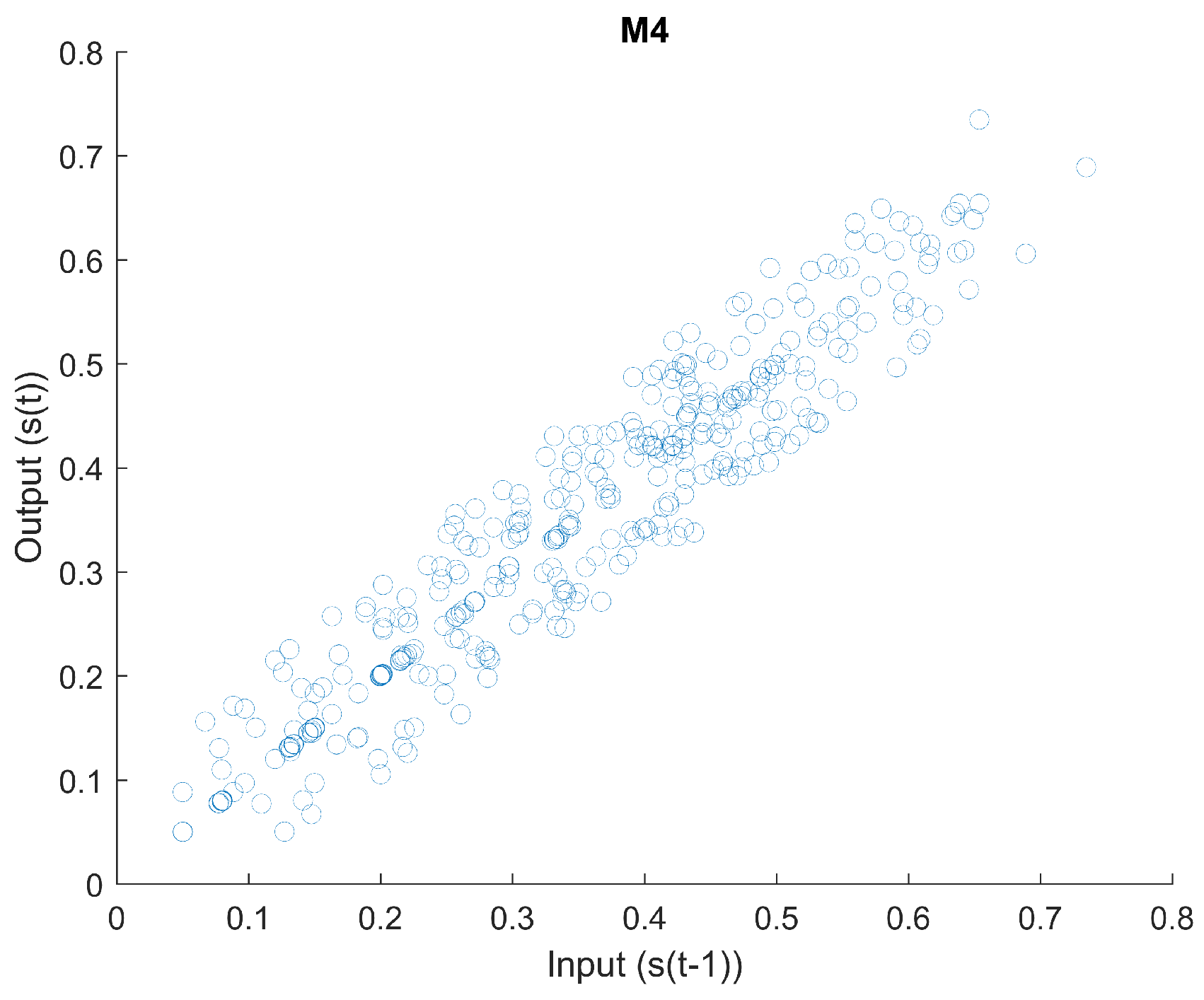
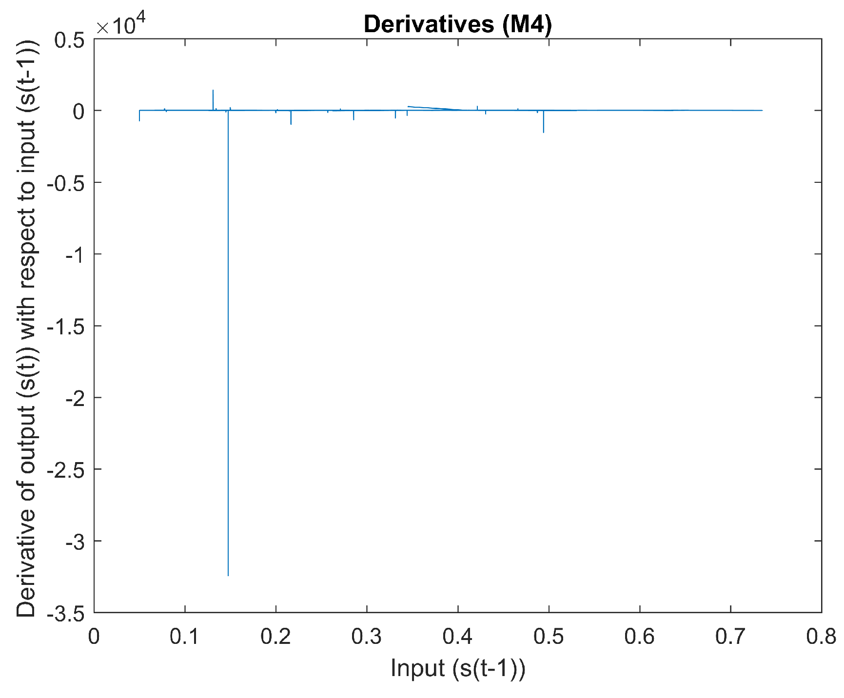
2.1.4. Mapping 4
Figure 12 is a scatter plot of input
vs. output
. The derivative of input
with regard to output
can be seen in
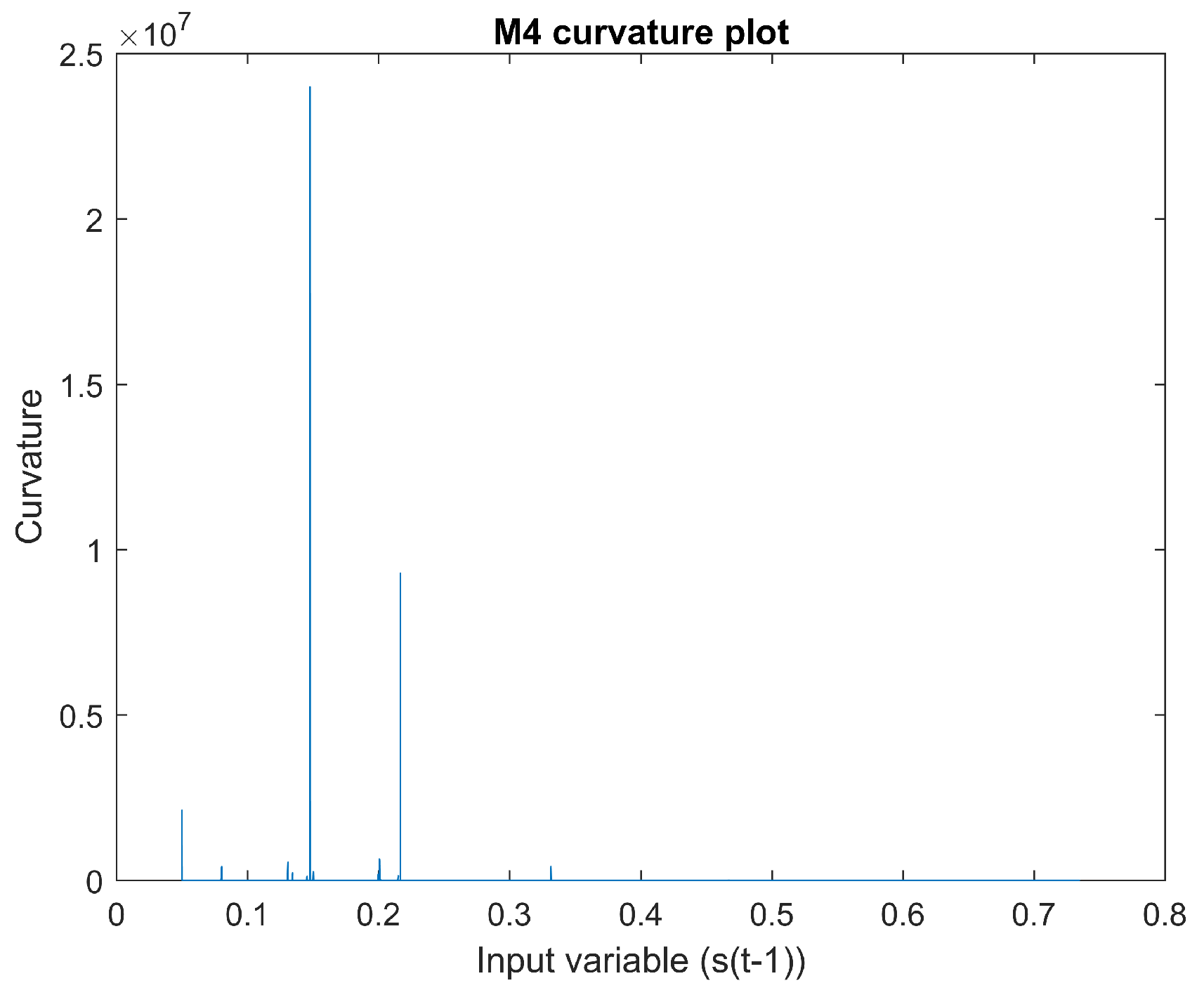
Figure 13. The curvature of this mapping can be seen in
Figure 14.
A lineal model, as described in Equation (
8), is another technique to analyze this mapping. The obtained adjusted
in this model is 0.9018; see
Table 7. Please notice that this time series, as will be shown in the next section, is not stationary. Hence, a direct implementation of a linear model is not appropriate.
2.2. Linear Approach
The variable that we are trying to forecast
is not stationary. This was formally tested with an augmented Dickey–Fuller test; see
Table 8.
Before using an ANN, it is advisable to use a lineal model. In order to do this, the three non-stationary variables and were made stationary by taking the differences: for example, using instead of . These variable transformations to make them stationary will be denoted with the operator “”. Hence, in the previous example , the stationary variable will be denoted as . The same notation is used for the speed. In this case, is denoted by . The target variable that we are forecasting follows the same notation (denoting .
Having a status of being non-stationary was once more tested using an augmented Dicker–Fuller test. As can be seen in
Table 9, now all the variables are stationary.
A linear model of the type shown in Equation (
9) can be tested.
The results of the linear regression are as follows (
Table 10). The multiple
and the adjusted
are 0.020230 and 0.009641, respectively.
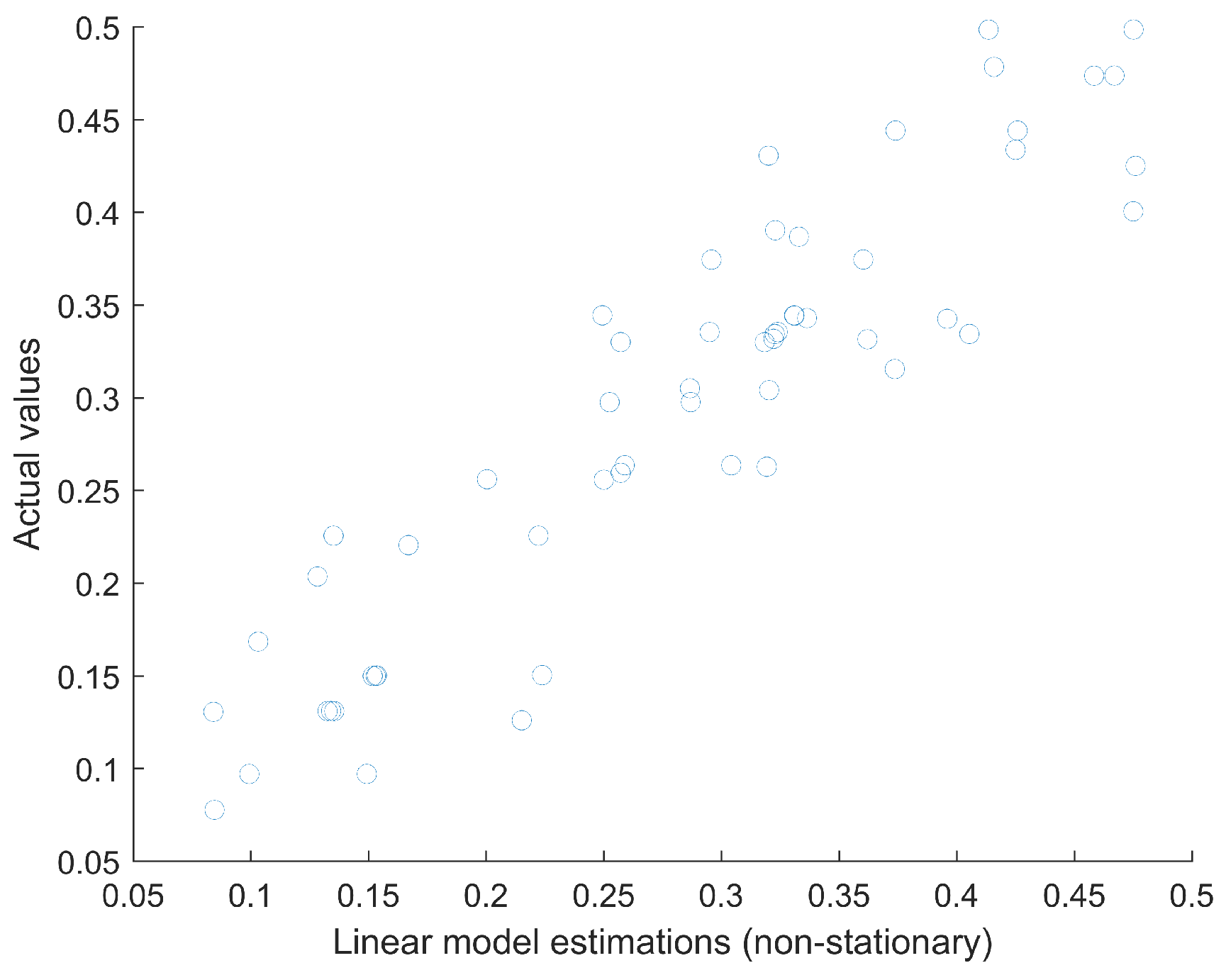
Lineal Model with Non-Stationary Data
If the lineal model is used with non-stationary data, then it is important for comparison purposes to use a similar approach to that in the ANN model that will be illustrated in the following section. For comparison purposes, a lineal model can be built, and then its generalization capabilities can be tested with 15% of the data (not used to build the linear regression). This approach is similar to the one followed in the next section. In this case, the obtained
(test data) is 0.8371 and the
is 0.0483. A scatter plot of the prediction of the linear model (using non-stationary data) and the actual values (test set) can be seen in
Figure 15.
2.3. ANN Approach
Authors such as Kim et al. [
55] have successfully applied ANNs to non-stationary data. Several other papers, such as Cheng et al. [
56], Ghazali et al [
57] and Marseguerra et al. [
58], also illustrate the application of ANN to non-stationary data. It is necessary to carry out an ANN parameter optimization task to try to make the estimated velocity
and the actual (measured) velocity
as similar as possible. There are several metrics
that can be used for this type of task, such as
or the
. In this case, we selected
as the metric to measure the similarity
of these values, but we also estimated the
. These metrics are impacted by the architecture of the neural network, such as the number of neurons
, the number of layers
and the training algorithm
used. This is an optimization problem that can be solved by using the Algorithm 1 shown below.
| Algorithm 1 An optimization problem |
- Require:
, and . - Ensure:
. - 1:
Compute for each configuration - 2:
Compare with for each configuration - 3:
Solve the following problem:
- 4:
Obtain , and
|
It should be noted that in this case, because the selected similarity metric is the comparing with , we have a maximization type of optimization problem. If we would have chosen the as the metric, we would have had a minimization problem. Additionally, it also should be explicitly mentioned that we are solving this problem using a grid approach. For each network configuration , there is an associated training process with a related training time, which is an important consideration. It will be shown that there is a non-linear relationship between the number of neurons and the time required to train such a neural network .
The use of ANNs also has its disadvantages. The initial weights in an artificial neural network are created randomly. This is an inherent part of the process. During the training phase, those weights are then modified to make the forecast as close as possible to the actual output (in this case, the velocity
). Because the weights are initially randomly generated, each ANN, even when having identical architectures (same number of neurons, layers and training algorithm), is likely to generate slightly different outputs. In order to reduce the impact of this initial random generation of the weights, each configuration is trained
times. The similarity values are the mean values of these
simulations for each ANN configuration. The
and the
reported are those obtained with the testing dataset. The testing dataset was not used during the training phase. After the ANN was trained, the testing data were used as input (no further training), the similarity metrics, such as the
and the
, were calculated, and the mean level was reported. We used a value of
equal to 100, i.e., each configuration
was simulated 100 times. The range for the number of neurons was
in increments of one neuron at a time. The hidden layers included neurons with a
transfer function as described in Equation (
10). The output layer consists of one linear transfer function.
Configurations with one to three layers were tested. Twelve different training algorithms were used (see
Table 11). Hence, 3276 different configurations were simulated (100 times each), for a total of 327,600 simulations.
Following this approach, the top 10 models were identified. After the model identification section, a robustness analysis was carried out. The robustness analysis consisted in simulating each of the ten top models identified in the previous section 1000 times. The batch size was 30.
2.4. Impact of Noise
We studied the goodness of the fit of the model when additional noise was added to the signal. Given the experimental challenges in achieving these measurements (at these scales), it is important to have an understanding of how well the model works when there is noise. This was tested by adding to the signal normally distributed noise
with mean zero (
) and
proportional to
of the original signal, according to Equation (
11).
where
is a parameter
. Several noise levels with zero means and increasing standard deviations were simulated. The standard deviations of the noise were increased from 1% to 100% of the standard deviation of the original signal in 1% increments. For each of these levels of noise, the model was simulated 100 times, and then, its goodness of fit was estimated using the
and
metrics. This process was repeated for all top 10 configurations obtained in the previous section.
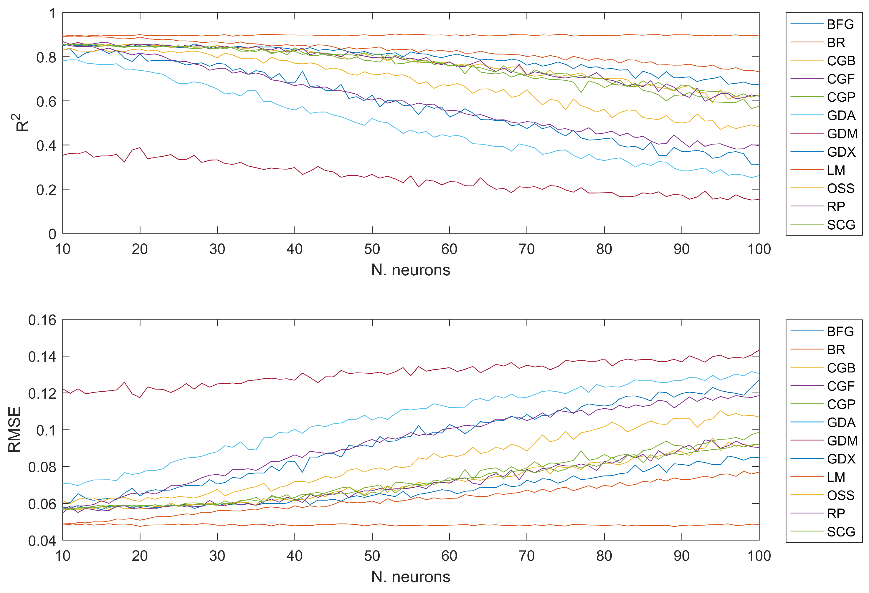
3. Results
As shown in
Figure 16 the selection of the training algorithm is important. All top ten models (highest
) use a BR (Bayesian regression) training algorithm and have only one hidden layer. In this table, both the
and the
are shown as a function on the number of neurons. As previously mentioned, the results reported are the mean values after 100 simulations for each configuration. Other models, such as GDM (see the abbreviations table at the end of the paper for a key to the names of the algorithms), generate much less accurate models. The top 10 models obtained are
. As an example, in this notation
, represents a model using 53 neurons in one hidden layer. There is no mention of the number of layers or the training algorithm in the notation because among the top 10 models, they all use the BR training algorithm and all have one layer. The best model obtained was
, with a mean
of 0.9029 and a mean
of 0.0476. A table with the results of all these 10 models can be seen in
Table A1 in the
Appendix A. The results for the most accurate models for all the other configurations (other training algorithms as well as models with two or three layers) can be seen in
Table A2 in the
Appendix A. All the reported data refer to the testing dataset, which was not used during the training phase and contains approximately 15% of the total data.
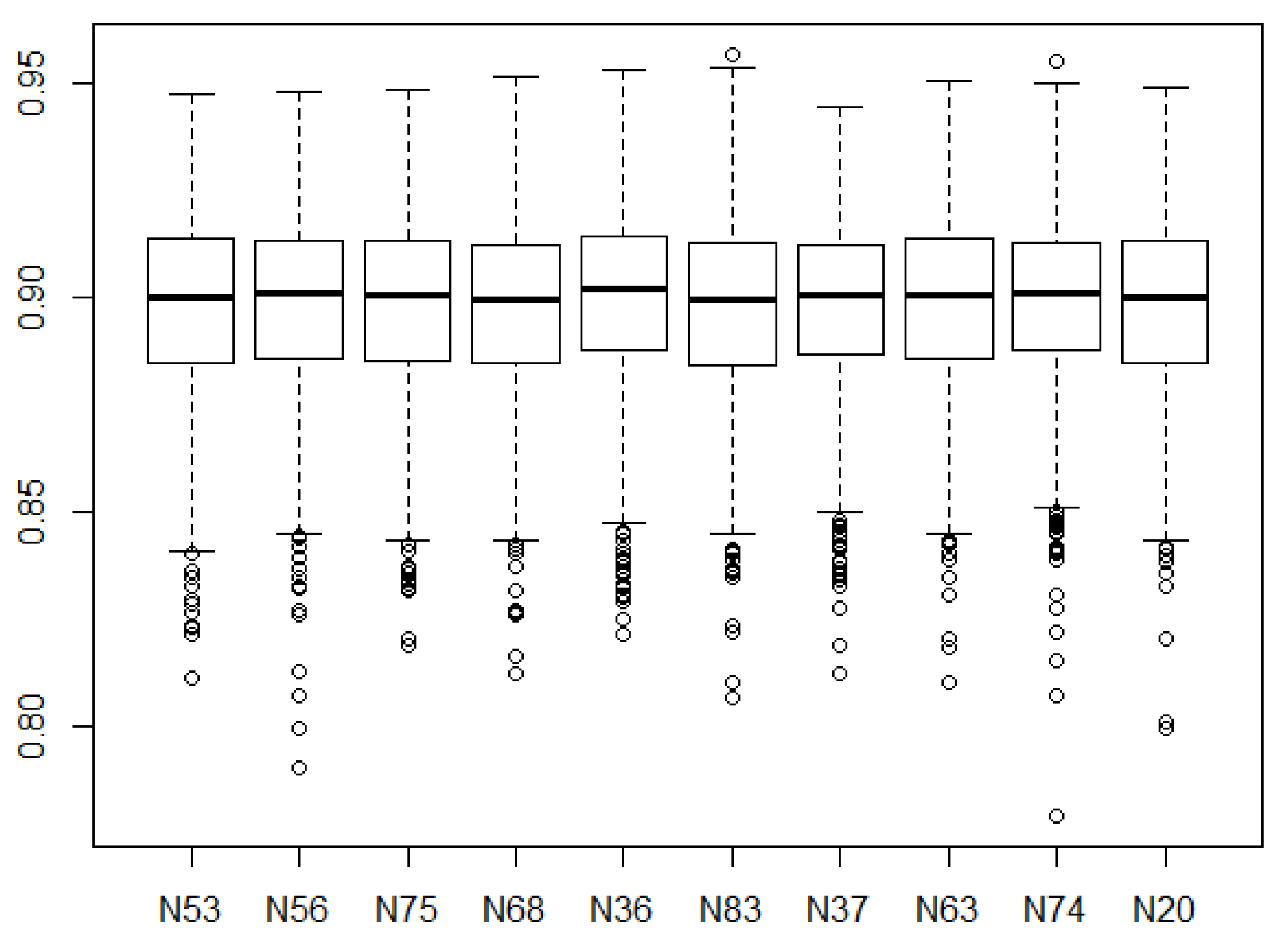
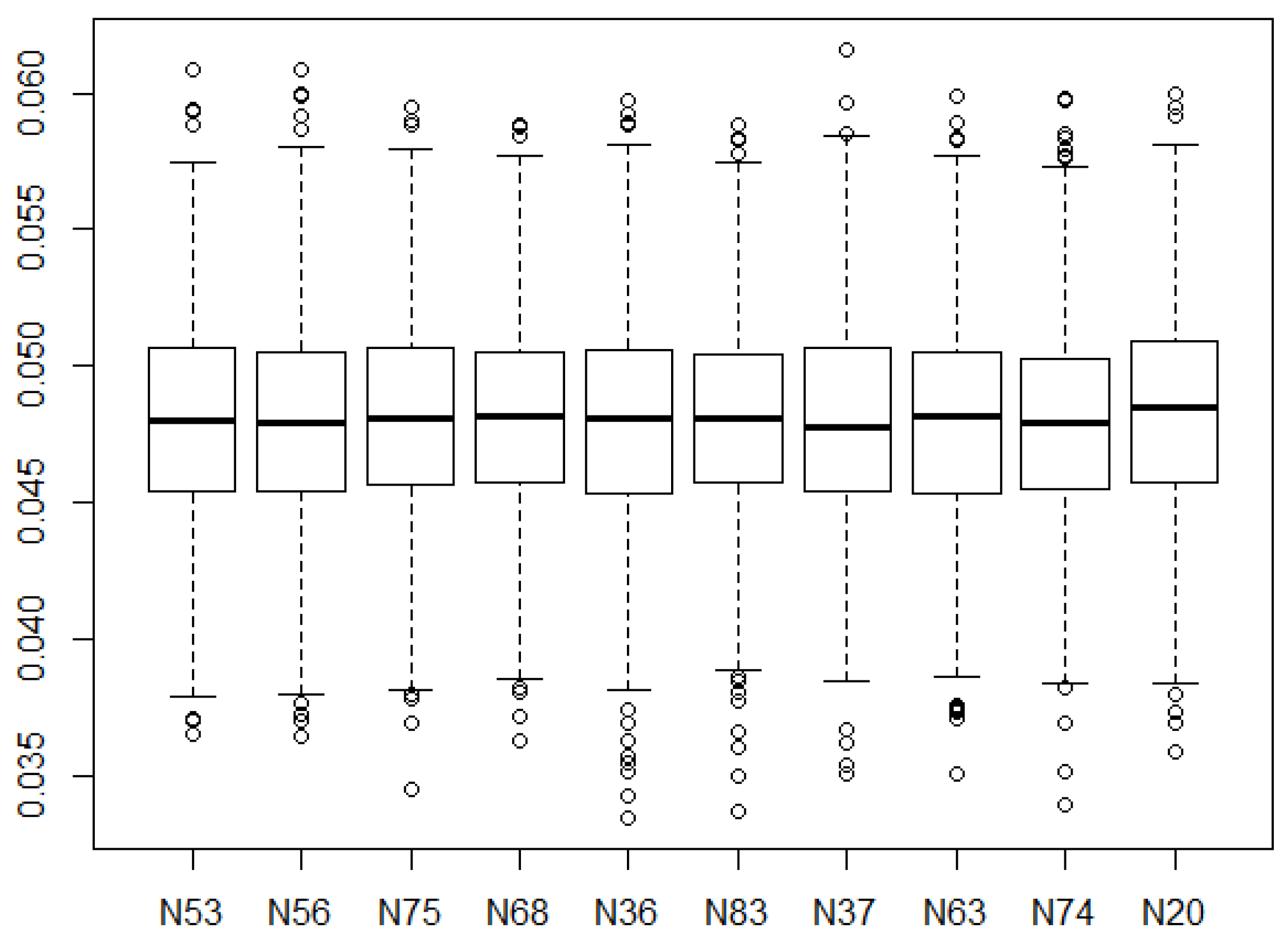
After the best 10 models were identified, it was necessary to carry out a robustness analysis. Each of these 10 top configurations were simulated 1000 times. The resulting
and
comparing the predictions of the testing dataset with the actual data were estimated for each simulation. The results (testing dataset) can be seen in
Figure 17 and
Figure 18. After the robustness analysis, the best model was N36 with a mean and a median
of, respectively, 0.8994 and 0.9017. The mean and median value for the
for this model were 0.0480 and 0.0481, respectively. For the same ANN configuration, the validation dataset obtained an
and
of 0.9150 and 0.0433, respectively. The results for all the 10 models (test dataset) can be seen in
Table A3 in
Appendix A.
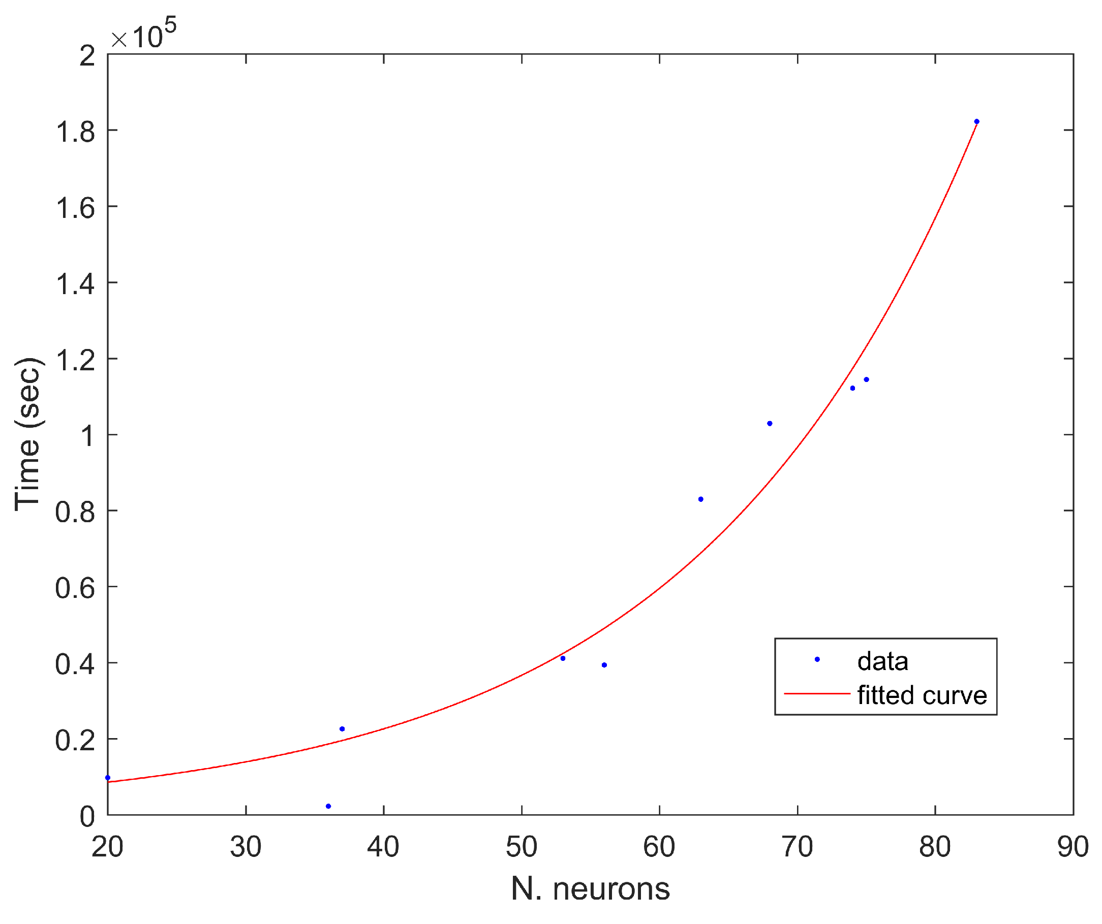
It also should be mentioned that the training time becomes an important factor to take into consideration. As the number of neurons increases, the related computational requirements increase. In the case of the robustness analysis (1000 simulations per configuration), the same non-linear relationship was observed (
Figure A1 in
Appendix A). In
Figure A1, it can be seen that the related training time increases (as we passed from 100 to 1000 simulations per configuration), but the shape of the curve remains similar, with an exponential increase in time as the number of neurons increases. The calculations were carried out in MATLAB on a laptop with an 11th Generation Intel i7-11700 @ 2.5 GHZ and 16 GB RAM.
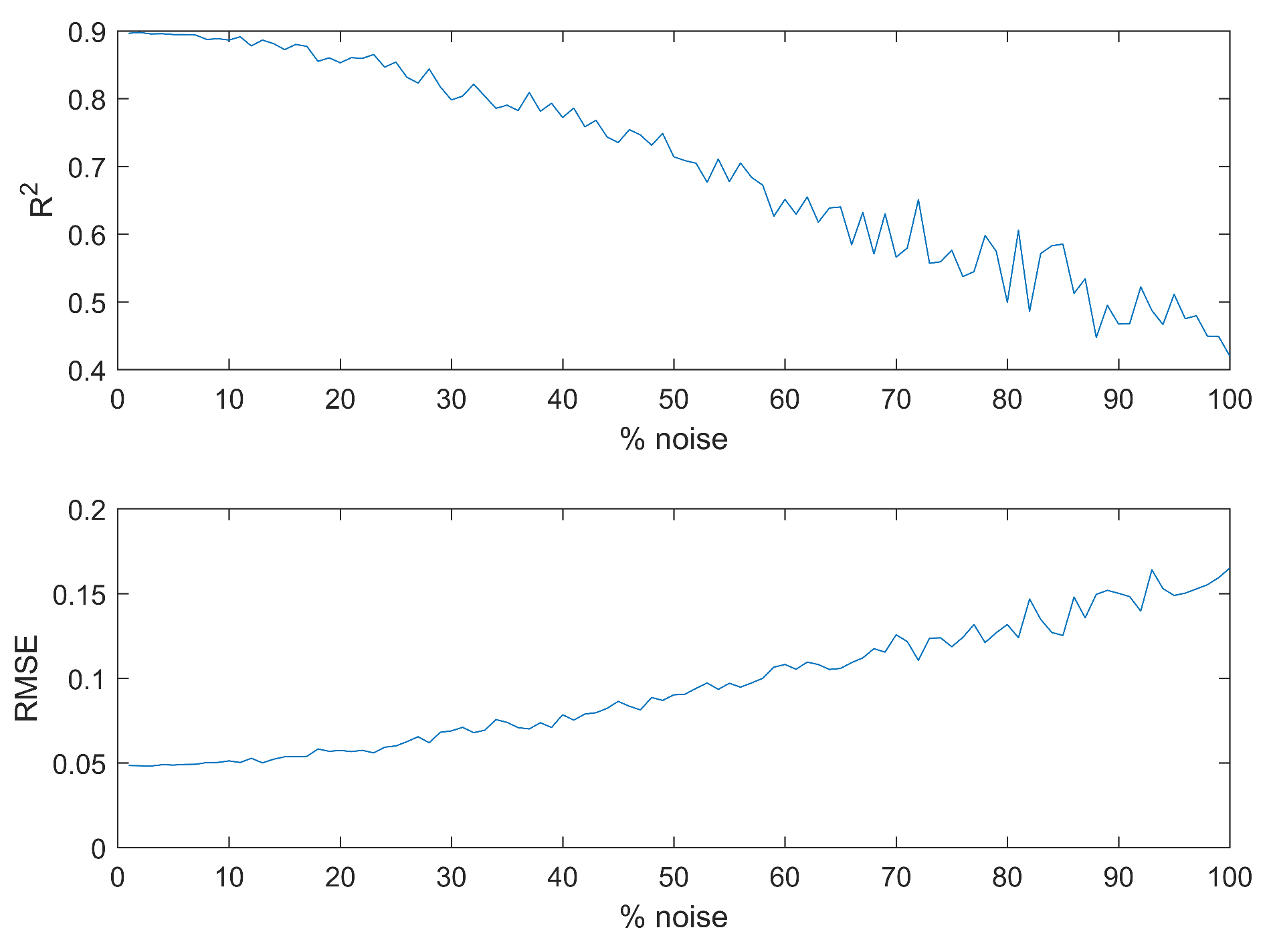
As can be seen in
Figure 19, when noise is added, the forecast velocity becomes less accurate. The bigger the
, the less accurate the forecast velocity becomes. As previously mentioned, the parameter
relates (according to Equation (
11)) the standard deviation (
) of the added noise with the standard deviation of the original signal (
). A value of
is 1% of the signal’s standard deviation, and
is 100% of the signal’s standard deviation. The
value comparing the forecast velocity and the actual velocity remains above 0.8 for
(33%).
4. Discussion
When analyzing the results, it should be taken into account that measuring blood microflows remains, from an experimental point of view, a challenging tasks. Not only are the scales involved small, but there are factors, such as the deformation of the red blood cells as they squeeze through the capillaries, that make the flow rather complex to model. There are also many different types of cells in the blood, further adding complexity to the model. Hence, there can be some inaccuracies in the measurements. In this regard, the model needs not only to be reasonably accurate but also robust and not too sensitive to noise.
The proposed ANN-based estimations (N53 configuration) obtained a mean
of 0.9029 and a mean
of 0.0476 in its estimations of blood velocity in capillaries (ranging from approximately 25 to 500
m). For comparison purposes, the configuration with the lowest mean
(0.512) was an ANN with two hidden layers and a GDM training algorithm (the results for all the configurations can be found in
Table A2 in
Appendix A). A total of 327,600 simulations were carried out in order to select an appropriate ANN architecture. The proposed grid approach selected a neural network with one hidden layer, 36 neurons and Bayesian regression (BR) as the training algorithm. Better performance of BR against other training algorithms has been observed in other applications [
59]. Deeper ANNs (with two or three layers) were not able to improve the forecasts generated by a one-layer structure. This highlights the need to select the appropriate network for the appropriate task, as blindly increasing the number of layers does not translate into a better model. This is likely due to overfitting. The importance of selecting the appropriate parameters in an ANN has been mentioned by several authors, such as Bernardos and Vosniakos [
60]. The selected model generated accurate forecasts when tested during the robustness analysis. When comparing these forecasts with the actual (measured) values of the velocity, the mean and median
were 0.8994 and 0.9017, respectively, while the mean and median value for the
were 0.0480 and 0.0481, respectively. These values were obtained by doing 1000 simulations with this final configuration. From a robustness analysis point of view it is always possible to do more simulations (in this case, we did 1000 per selected model). However, given the similarity of the results for the top 10 selected models, it would appear that 1000 iterations is likely a reasonable amount, particularly when considering the computational cost when substantially increasing the number of simulations per configuration. The BR training algorithm appears to consistently outperform all the other training algorithms tested (12 in total). Similarly, there were some training algorithms that consistently underperformed, such as GDM, GDA and the GDX. The best results using two hidden layers were obtained for the BR training algorithm, with a mean
value of 0.8992. This value was obtained with 100 simulations; using the same number of simulations, the one-layer model obtained a mean
of 0.9029 (which slightly decreased to a value of 0.8994 after the robustness test using 1000 simulations). The worst result using a two-layer configuration was obtained using the GDM algorithm (
of 0.512). When using three layers, the best results were obtained with the Levenberg–Marquardt training algorithm, with a mean
of 0.860. Similarly to the two-layer case, when using three layers, the worst results were obtained when applying the GDM training algorithm (
of 0.510). The top 10 models obtained using the grid approach generated comparable results. Even after the robustness analysis, these 10 models seemed to perform roughly in a similar fashion (see
Figure 17 and
Figure 18). These ten models generated forecasts that are statistically significantly better than those obtained with different ANN architectures.
It was observed that the computational time required to train the network increased non-linearly with the number of neurons. This was observed during the model selection phase as well as during the robustness analysis. While the computational times required in these two sections were different (in one case, there were 100 simulations per ANN configuration, and in the other case, there were 1000) the shape of the curve representing computational time vs. the number of neurons was similar (exponential curve). Given this observation and the fact that models with more neurons did not necessarily perform better, it highlights the need for adequate ANN parameter selection. Computational time is an important factor, with some training processes requiring more than a day for a single configuration. This limits the total number of testable configurations. These computational times were obtained using standard laptops, and hence, with more computational power, these training times could be reduced. Another additional consideration is that the exponential trend was observed within a particular range of neurons. It was not tested with more than 100 neurons per layer.
It was also interesting to see the performance of the model when introducing noise in the signal. The introduced noise was normally distributed with zero mean and a standard distribution proportional to the original standard distribution of the signal (in 1% increments from 1% to 100%). The model managed to generate accurate forecasts, with a mean above 0.8, until reaching 33% of the standard deviation of the original signal. This type of analysis, adding some artificial noise to the signal, was carried out in order to better understand how well the model reacts to noise. This is important, as measurements in the analyzed scale are experimentally difficult to obtain and could have, in principle, substantial error that might be difficult to estimate. The model seems adequate for the above-mentioned levels of noise (less than 33% of the standard deviation of the original signal). If there are indications that the noise is bigger than that, then the proposed model might not be accurate enough. The precision of the presented model is high (with an of 0.8992). The usefulness of this model to other researchers will depend on their required precision. While the scale of the analysis is likely enough for many pharmaceutical applications, in some instances, there might be a need for higher precision. This would require not only further improvements in the modeling but also more precise experimental data, which can be challenging to obtain.
Kloosterman et al. [
54] mentioned that a vascular network approach can be used to investigate vascular development. They also concluded that vascular remodeling could be observed, and that the changes in network parameters, such as the velocity, could be related to structural changes. The authors also mentioned that some networks became denser, but other networks became less dense.


