Discharge Capacity Estimation for Li-Ion Batteries: A Comparative Study

Abstract

Li-ion batteries are integral to various applications, ranging from electric vehicles to mobile devices, because of their high energy density and user friendliness. The assessment of the Li-ion state of heath stands as a crucial research domain, aiming to innovate safer and more effective battery management systems that can predict and promptly report any operational discrepancies. To achieve this, an array of machine learning (ML) and artificial intelligence (AI) methodologies have been employed to analyze data from Li-ion batteries, facilitating the estimation of critical parameters like state of charge (SoC) and state of health (SoH). The continuous enhancement of ML and AI algorithm efficiency remains a pivotal focus of scholarly inquiry. Our study distinguishes itself by separately evaluating traditional machine learning frameworks and advanced deep learning paradigms to determine their respective efficacy in predictive modeling. We dissected the performances of an assortment of models, spanning from conventional ML techniques to sophisticated, hybrid deep learning constructs. Our investigation provides a granular analysis of each model’s utility, promoting an informed and strategic integration of ML and AI in Li-ion battery state of health prognostics. Specifically, a utilization of machine learning algorithms such as Random Forests (RFs) and eXtreme Gradient Boosting (XGBoost), alongside regression models like Elastic Net and foundational neural network approaches including Multilayer Perceptron (MLP) were studied. Furthermore, our research investigated the enhancement of time series analysis using intricate models like Convolutional Neural Networks (CNNs) and Recurrent Neural Networks (RNNs) and their outcomes with those of hybrid models, including a RNN-long short-term memory (LSTM), CNN-LSTM, CNN-Gated Recurrent Unit (GRU) and RNN-GRU. Comparative evaluations reveal that the RNN-LSTM configuration achieved a Mean Squared Error (MSE) of 0.043, R-Squared of 0.758, Root Mean Square Error (RMSE) of 0.208, and Mean Absolute Error (MAE) of 0.124, whereas the CNN-LSTM framework reported an MSE of 0.039, R-Squared of 0.782, RMSE of 0.197, and MAE of 0.122, underscoring the potential of deep learning-based hybrid models in advancing the accuracy of battery state of health assessments.

1. Introduction

Li-ion batteries (LIBs) are widely used in different areas due to their high energy capacity, fast charging, and light weight. The performances of LIBs, which are considered the best energy storage systems for electric vehicles, are gradually decreasing due to their chemical and physical mechanisms [1]. An efficient battery management system needs to be developed due to high costs and limited repair opportunities. Moreover, in order to effectively manage the performance of batteries, the health indicators of the battery must be accurately predicted. Therefore, it is very important to estimate the state of health (SoH) of batteries and monitor their life cycle for long-lasting and high-performance battery use.

In the quest for advancing battery technology, the incorporation of symmetry plays a crucial role in the analysis of Li-ion batteries. Symmetry, embodying balance and harmonious patterns, has been systematically explored to unveil inherent structural regularities within battery data. Investigating symmetrical properties provide a detailed comprehension of the fundamental mechanisms governing battery operation. This, in turn, contributes to refining existing models and fostering the development of more resilient battery management systems.

Data-driven methods are being developed to analyze the dynamic behavior of a system without investigating the electrochemical reactions that occur during the battery discharge time. The data of raw measurements obtained from actual battery usage experiments are utilized to analyze the dynamic behavior. Abundant data are needed for the training of the models developed for these methods. For testing operations, the unused data in training is provided as input to the model for the testing process, so this is performed in data-based methods and statistically based approaches. In different studies, a fuzzy logic theory has been used to predict the SoH of LIBs [2]. Moreover, in [3], a Genetic Programming (GP)-based approach was developed to extract the optimal formula for the SoH prediction of batteries. A hybrid model developed in [4] combines a Support Vector Machine (SVM) with an Unscented Particle Filter (UPF) to improve the performance of the SoH and state of charge (SoC) predictions in LIBs. In [5], an adaptive Wiener process model using the Brownian motion process for RUL (remaining useful life) estimation was proposed. Machine learning (ML) algorithms have received particular attention due to their outstanding performance and minimal prediction errors. Cai et al. proposed a prediction model using Support Vector Regression (SVR) for battery SoH prediction; a Genetic algorithm was employed to optimize SVR parameters and feature selection [6]. Xue et al. proposed a hybrid approach, a combination of an Adaptive Unscented Kalman Filter (AUKF) and SVR, for the remaining useful life (RUL) prediction of LIBs. SVR parameters were optimized using a genetic algorithm [7].

In general, data-driven methods achieve superior accuracy than model-based methods. Recently, research on improving the battery state estimation accuracy has shown significant success. Several studies have conducted comparative analyses between machine learning algorithms to predict the internal states of LIBs. For instance, a comparative study of different machine learning algorithms such as SVR, Convolutional Neural Networks (CNNs), and Long Short-Term Memory (LSTM) was conducted in [8].

In recent years, hybrid methods have been introduced to leverage multiple algorithms to increase the precision of a prediction method. Further studies have suggested a combination of LSTM networks with other methods to improve the prediction accuracy and achieve the best results. Liu et al. combined LSTM with Bayesian Model Averaging (BMA) for RUL estimations [9]. In a different study, the performance results of the proposed GPR and LSTM methods were compared separately with the performance of Gaussian Process Regression—Empirical Mode Decomposition (GPR-EMD) and an LSTM-EMD combination [10]. Convolutional neural networks play a crucial role in feature mapping. Combining CNN and LSTM networks increases the adequacy of diagnosis and prognosis methods. Several studies have proposed a combined CNN-LSTM to improve the prediction accuracy and overcome the performance degradation of batteries. Ren et al. applied a hybrid CNN-LSTM model for battery RUL prediction [11]. The method performed well using a limited amount of data in the learning phase, and the prediction errors were satisfactorily small [12]. In addition to all these methods, our research team discussed enhancements to the LSTM (long short-term memory) and Bi-LSTM (Bidirectional Long Short-Term Memory) methods. Evaluation metrics such as the Mean Squared Error (MSE), Mean Absolute Error (MAE), Root Mean Square Error (RMSE), and R-squared were applied in our previous publication [13].

Recent studies on data-driven methodologies underscore a pivotal shift toward leveraging comprehensive raw measurement datasets from actual battery usage to analyze dynamic system behaviors, bypassing the need to investigate the intricacies of electrochemical reactions during discharge. These methodologies necessitate substantial data volumes for model training, ensuring that the predictive models are robust and generalizable. In the literature, the adoption of machine learning algorithms, particularly when optimized with genetic algorithms, has been shown to significantly reduce prediction errors. Comparative analyses have elucidated the superior efficacy of these data-driven approaches over traditional model-based methods, particularly highlighting the effectiveness of hybrid models that combine CNN and LSTM networks to enhance feature extraction and sequential data analysis. Such synergistic models are shown to be crucial in improving the predictive accuracy and reliability of battery status estimations.

This study focused on analyzing the change in the discharge capacity of LIBs over time and developing predictive models to anticipate capacity decline. In addition to analyzing the change in the discharge capacity of LIBs over time, it aimed to develop predictive models that predict the capacity decrease by taking into account the concept of symmetry. For this goal, LIBs were charged/discharged, and discharge capacity values were obtained by adhering to different temperature and charge/discharge procedures. Afterward, various modeling approaches were explored, ranging from classical machine learning algorithms to complex and hybrid deep learning models. The performances of algorithms such as Random Forests (RFs) [14] and eXtreme Gradient Boosting (XGBoost) [15] were evaluated alongside regression models like Elastic Net [16] and artificial neural network models like Multilayer Perceptron (MLP) [17].

Furthermore, efforts were made to improve success rates in time series data analysis by developing more sophisticated models. Complex architectures such as CNNs and Recurrent Neural Networks (RNNs) were developed and compared within hybrid frameworks like RNN-LSTM, CNN-LSTM, CNN-Gated Recurrent Unit (GRU), and RNN-GRU. This comprehensive approach aimed to enhance our understanding of battery behavior and facilitate the creation of more accurate prediction models for BMS applications for determining the critical indicators of its aging status, which can be identified through factors like increased internal resistance or diminished capacity. By effectively monitoring and assessing these parameters, the BMS contributes significantly to maximizing battery performance and longevity.

Unlike the hybrid methods mentioned in the literature, the methodology proposed in this study provides researchers with a comparative analysis by outlining the feature exploitation procedure for classical machine learning and two neural networks (CNN, RNN). Therefore, for future studies, it elucidates which method will obtain more accurate and faster results. Additionally, a comparison of the LSTM algorithm and GRU algorithms was conducted to demonstrate the superiority of the proposed method. A CNN was combined with an LSTM network for the SoH estimation and RUL assessment of LIBs. Improving the proficiency of machine learning algorithms has always been a subject of research. However, among these attempts, several studies have proposed more complex RNN combinations [18]. Comparative results of an LSTM and GRU-based hybrid CNN and RNN methods are included in the study to demonstrate the superiority of the proposed methods. To compare observed and predicted discharge capacities, evaluation metrics such as the MSE, MAE, RMSE and R-Squared were applied to the proposed methods [19].

The remainder of this paper is structured as follows; in the second section, the materials and methods used are provided. In the third section, the LIB data preparation is first discussed and then presented. The data were analyzed from different perspectives. In the fourth section, based on data analysis, various (RF, XGBoost, Elastic Net, MLP, CNN, RNN, CNN + LSTM, RNN + LSTM, CNN + GRU and RNN + GRU) models for LIB discharge performance were proposed with machine learning and deep learning techniques. In the following sections, the models are evaluated and compared in detail. Finally, the study concludes by providing results and recommendations. Additionally, the limitations and findings of the study are included. Thus, researchers are given predictions for future studies.

2. Materials and Methods

This study aimed to examine the performances of different prediction methods as a step toward improving the LIB discharge capacity prediction. These methods include various approaches such as machine learning and deep learning. This comparative study discusses the advantages, disadvantages, and application areas of each method in detail and sheds light on the future development of LIB technology.

Test outcomes acquired under four distinct temperatures, two diverse discharge capacities, and two varying charge cut-off current values can be utilized to instruct machine learning models in discerning data, such as capacity and voltage, for alternative charge/discharge currents and temperature values.

2.1. Battery Tests

All the tests were obtained from open-access sources from Michael Pecht, Centre for Advanced Life Cycle Engineering (CALCE), University of Maryland. The experiments were described to be conducted with LiCoO₂–Graphite cells [20].

All the charge/discharge tests were described to be conducted in the operation range of 3.0–4.4 V with different C-rates and temperatures. The number of cells and test parameters are shown in

Table 1. Test parameters applied to cells [20].

Discharge	Ambient Temperature (°C)				Charge Cut-Off
C-Rate	10	25	45	60	C-Rate
0.7 C	Test No.1	Test No.7	Test No.13	Test No.19	C/5
	Test No.2	Test No.8	Test No.14	Test No.20	C/40
1 C	Test No.3	Test No.9	Test No.15	Test No.21	C/5
	Test No.4	Test No.10	Test No.16	Test No.22	C/40
2 C	Test No.5	Test No.11	Test No.17	Test No.23	C/5
	Test No.6	Test No.12	Test No.18	Test No.24	C/40

. Every test condition (Test No.1, No.2, etc.) consists of 8 cells with a total of 192 cells. Every eight cells applied four different temperatures, three different discharge C-rates, and two different charge cut-off C-rates with C/5 and C/40 following the constant charge–constant voltage (CCCV) protocol. Machine learning techniques were utilized to train models using all obtained charge and discharge datasets. These datasets served as input for the training process, enabling the models to learn and predict outcomes based on historical data patterns.

2.2. Random Forrest (RF)

RFs, random decision forests, is a machine learning method for classification and regression that works by performing a large number of decision trees. RF can be described as a combination of decision tree algorithms. It has the ability to improve the accuracy of the information in a single tree with information from many trees. RF eliminates over-reliance on training data, and it presents successful results within a large amount of data. Therefore, it is commonly used in many areas [14].

The RF technique combines the bagging technique with the random subspace technique. It was preferred by Breiman in 2001 over the bagging method because it provides more randomization [21]. It is an algorithm with a lower margin of error and, accordingly, a higher predictive power. This technique consists of randomly selected decision trees from the original dataset. Different sets are created from the decision tree dataset through bootstrapping. In total, 2/3 of the dataset is reserved as a learning dataset (in bag) and 1/3 as a test dataset (out of bag).

In RF, estimation is also performed for the data that is introduced later. Calculating the importance of variables has also become an advantage for RF, especially if the dataset contains many variables. The number of trees to be created and the number of variables to be selected are very important in this technique. Other factors will not change the result much [21].

2.3. XGBoost Algorithm

The XGBoost algorithm is an efficient and widely used integrated learning method proposed by Dr. Tianqi Chen from the University of Washington, based on Gradient-Boosted Decision Trees (GBDTs) and RF. It can be applied to both classification tasks and regression problems. Compared with GBDT and RF, XGBoost not only has better accuracy, but also provides a parallel tree-boosting structure that solves many data science problems quickly and accurately [22].

XGBoost is a tree model consisting of multiple decision trees (CART: Classification and Regression Tree). The first step in XGBoost is to make the initial estimate (base score). This estimate can be any number, as the correct result will be reached by converging with the steps to be taken in the next steps. This number is 0.5 by default. In the next stage, a decision tree that predicts errors is established, as in Gradient Boosting. The aim here is to learn from the mistakes and get closer to the correct prediction. The prediction is examined using the erroneous predictions (residuals) of the model. Errors are found by subtracting the predicted value from the observed value. The predicted values of all decision trees are summed as the final result, and multiple weak learners are integrated into a strong learner using certain methods. The splitting process of a single decision tree in XGBoost is the same as that of a CART regression tree, except that the objective function used is different. The objective function of each tree is given in Equation (1):

$$OBJ={\sum }_{i=1}^{n}l\left(y_i,{\widehat{y}}_i^{\left(t-1\right)}+f_t\left(x_i\right)\right)+\Omega \left(f_t\right)$$

(1)

The objective function has two components. The first is the loss function, which is employed to evaluate the loss or error between the model’s predicted value and its actual value. The second component is the regularization term utilized to control the complexity of the model. The regularization term tends to select simple models to avoid overfitting [23]. This prevents the overfitting of a model to its training data. An attempt is made to eliminate a situation that causes a decrease in performance against new and unseen data. This prevents overfitting and makes the model more generalizable. Thus, successful results can be obtained in dense time series data such as those of LIBs.

2.4. Elastic Net

Elastic Net is a linear regularization and variable selection method that was proposed to deal with the disadvantages of the Lasso and Ridge estimators by Zou and Hastie in 2005 [24]. Elastic Net was developed as a solution to the Lasso approach, which can be unstable in the case of multiple types of data. The Lasso and Ridge estimators realize variable selection and analysis; accordingly, Lasso makes irrelevant values zero, while Ridge brings the values of irrelevant variables in the data closer to zero. Ridge regression can be used while analyzing multivariate data. This is to keep the error value to a minimum by finding the coefficients that make the sum of squares zero. Elastic Net consists of a combination of the Ridge and Lasso estimators [25]. It is established on a combination of l1 (Lasso estimator) and l2-norm (Ridge estimator) penalization. Figure 1 shows these three methods together. The outermost circular line is the Ridge approach, while the central square pattern indicates the Lasso approach. The orange line between the two approaches is a representation of Elastic Net.

The regression type with two parameters $\left(a,\lambda \right)$ for adjustments can yield a more efficient result. $a$ is a hyperparameter for controlling the balance between the Ridge and Lasso estimators. If $a=0$, there is a relationship between the Elastic Net and Ridge estimators. If $a=1$, there is a relationship between the Elastic Net and Lasso estimators. $\lambda$ is a tuning parameter that detects an amount of regulation. Although Lasso ignores datasets with similar relationships, Elastic Net continues to reach saturation in case of multiple data. It is an attractive method due to its high predictability and easy interpretation [26].

2.5. Multilayer Perceptron

The perception model is an artificial neural network model. Since it is a supervised learning algorithm, both input and output data are input to the network. One of the most important points for the perceptron model is the threshold value. If this value is suitable for the desired data, the model provides more accurate results. In this process, the learning ability is improved by increasing the number of iterations [26].

Figure 2 shows a single-layer perception. The $x$ values represent the inputs, the $w$ values represent the weights, and then the net input is calculated. The output value is determined as zero if the input is below the threshold, and the output value is one if it is higher.

An MLP contains more hidden layers, unlike the single perception model. Multilayer networks consist of the input layer, one or more hidden layers, and output layers, and a high number of neurons in the hidden layers reduces the error rate. In this method, the network is trained with samples, and the network determines the output result accordingly [27]. After the sample is trained between the input and hidden layers, it is transferred to the output layer when the error is the lowest value. The Delta learning method is employed in the MLP. The number of middleware depends on the complexity of the problem. Any of the sigmoid, tang, linear, threshold and hard limiter functions can be used as the activation function in this model [28].

2.6. Convolutional Neural Networks

CNNs are deep learning models designed especially for image recognition and processing tasks [29]. Time series data, which can be viewed as a 1-dimensional grid with regular time intervals, and image data, which can be viewed as 2-dimensional pixels, can be successfully processed with CNNs. CNNs consist of various layers, including an input layer, convolution layer, pooling layer, ReLU layer, fully connected layer, and output layer. The input layer receives the data and passes it to the convolution layer. In this layer, filters are utilized to extract targeted nonlinear models from the input data, resulting in feature maps. The pooling layer is utilized to downsample these feature maps. Then, the pooling layer converts the multidimensional shape of the feature maps into a one-dimensional shape and then sends it to the fully connected layer. The fully connected layer calculates the final results based on these features [30,31]. Figure 3 shows an example of a CNN used for time series forecasting, where a univariate time series is used as input, and the output represents a forecast.

This architecture was designed to predict a given time series data point $X_t,X_{t+1},\dots ,X_{t-k+1}$ based on data from past time steps. A convolution layer is used to extract local features by applying a series of filters on the data received from the input layer. In this layer, the feature maps obtained as a result of each convolution process represent different aspects of the input. The output of the layer is a combination of features that better represent the time series patterns in the original dataset.

2.7. Recurrent Neural Networks

An RNN is a type of deep learning architecture and is called a recursive neural network [18]. In neural networks other than RNNs, inputs are handled independently of each other. The order in which the inputs arrive in the network does not matter. After the processing of the input in the network is completed and the output is produced, the neural network forgets the input. In areas such as image processing, one input can be provided at a time. However, data such as weather cannot be input to the network at once. For this reason, RNNs, which are neural networks with memory, have been produced as a solution. RNNs progress by keeping the information of the previous data in memory while training the network. Therefore, it can be successfully used in SoC predictions of LIBs containing time series data. SoC time series data provided to an RNN are processed step by step in the inner loop of the network, and an output is produced. During this process, information from the previous layer (hidden state) is updated and transferred to the next layer through repeating layers. Figure 4 shows the internal structure of the RNN architecture.

In the internal structure shown in Figure 4, $x_0$ takes the input and combines it with the hidden state, produces an output, and then updates the hidden state. Meanwhile, it takes the input $x_1$, the current input, and the hidden state and sends it as input to the other layer. After all these processes are completed, the hidden state is updated again. This structure enables more accurate predictions about the future without forgetting past experiences.

2.8. Long Short-Term Memory

In examining an RNN, it is seen that predictions for the future are made using past experiences. If transactions are made within a large network and we are trying to process a long paragraph or history-dependent data, the value we will obtain will increase exponentially. This may cause an increasing gradient explosion. As a solution to this problem, LSTM [18] and GRU [31] models, which are specialized versions of RNNs, have been proposed. The LSTM network architecture consists of four neural networks and special memory blocks known as cells. By default, the LSTM network is designed to retain information for long periods of time. Operations in the LSTM are performed by three gates. The first of these is the forgetting gate $\left(f_t\right)$, the second is the entry gate $\left(i_t\right)$, and the last is the exit gate $\left(i_t\right)$. These gates determine the importance of information and decide what should be kept or discarded. LSTM cell consists of two main blocks. The first of these is the cell state $\left(C_{t-1}\right)$ and the hidden state $\left(h_{t-1}\right)$. These states are constantly updated and carry information from previous time steps to the present. While the cell state acts as a store for long-term memory, latent states serve as a store for short-term memory. The architectural structure of an LSTM network is shown in Figure 5.

2.9. Gated Recurrent Unit

A GRU neural network is an improved model of an RNN that exhibits superior long-term sequence memorization capabilities compared to the standard RNN. It functions similarly to LSTM in solving the gradient explosion or disappearance problem of simple RNNs. Unlike LSTM, in GRU, the forget and input gates are synthesized into a single update gate and only one hidden state is processed to transmit information. A GRU can be thought of as a different version of LSTM with an easier design, fewer variables, and higher convergence. The GRU base unit consists of an update gate and a reset gate. The update gate decides how much of the new candidate state should be added to the existing hidden state. The output of the previously hidden layer has a large impact on the current hidden layer. The purpose of the reset gate is to manage how much of the previously hidden state should be forgotten; a smaller value indicates that more information has been ignored, thus reducing the dependence on past information. The basic architecture of a GRU is shown in Figure 6.

3. Experimental Studies

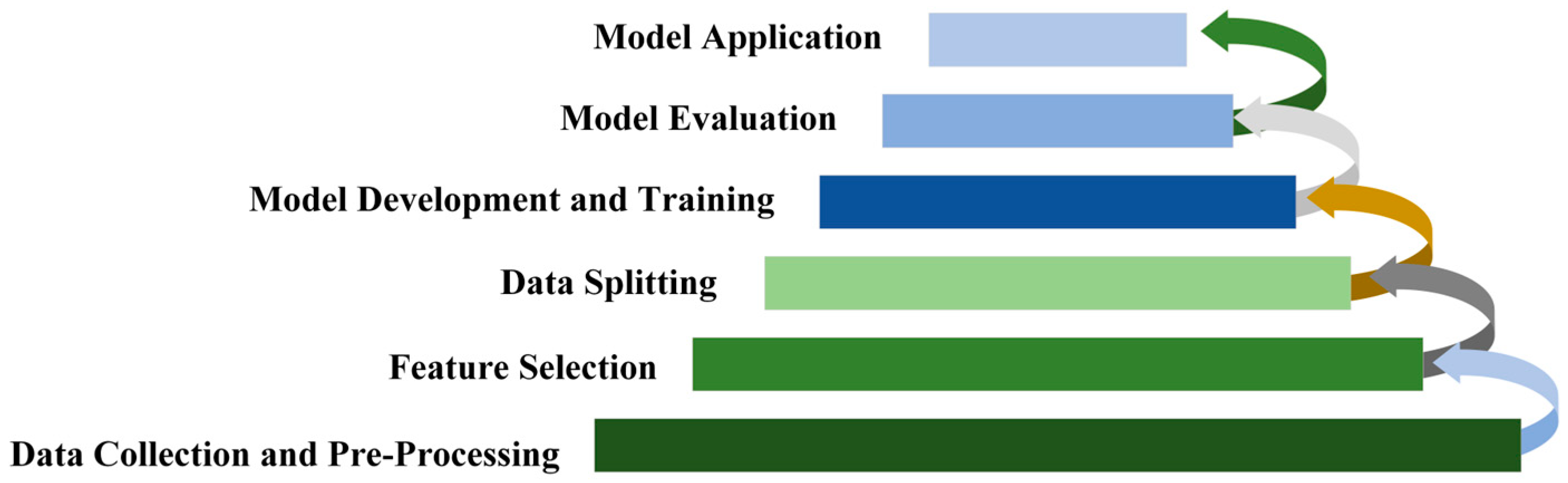
Within the scope of this study, various models were developed to estimate the discharge capacities of LIBs, each employing distinct computational strategies. The initial deployed model was based on the RF algorithm, a well-established machine learning technique. Subsequent models included those based on XGBoost, CNNs, RNNs, and integrated frameworks that combine CNN and RNN units with a GRU and LSTM to harness their respective strengths. The development of these models was meticulously structured, adhering to a prescribed sequence of steps. During the model development phase, the methodologies and procedural stages were rigorously followed as outlined in Figure 7, ensuring systematic progression and integrity in the model development.

The process of developing a predictive model, as depicted in Figure 7, commences with the gathering and pre-processing of historical data pertinent to the predictive task, such as discharge capacity data. This foundation is followed by feature selection, where key data attributes are identified to accurately predict the outcome variable. Afterward, the dataset is partitioned into distinct training and testing sets. The training set informs the model learning phase, which varies according to the algorithm employed—a subject extensively covered in the Materials and Methods section. The model performance is then assessed on the test set, employing metrics like the RMSE to ascertain the predictive accuracy. The finalized model, upon validation, becomes a tool for real-world application, capable of forecasting outcomes on novel data, thereby enabling empirical studies on actual data scenarios.

3.1. Data Collection and Pre-Processing

Table 1 presents the cycling test structure involving temperature, charge cut-off C-rate, and discharge C-rates; three stress factors that resulted in 24 testing conditions. Each condition was subjected to testing using eight cells. All cycling data were logged by the battery test system and were pre-processed for machine learning and deep learning purposes.

Pre-processing was applied to the obtained data, and missing values were checked. Scaler transformation was applied to the data for artificial intelligence algorithms. Features at different scales may cause the algorithm to over- or under-react to certain features, so an attempt was made to normalize values that may become more dominant in model training. Additionally, in deep learning models, the normalization of features helps train the model faster and more effectively. Normalization enables optimization algorithms such as gradient descent to converge faster and more effectively.

In working with deep learning models used in structures such as time series, image processing, or sequential data, the need to transform the data into a three-dimensional tensor is necessary to make the data suitable for the input format expected by the model so that the model can process the data correctly and learn effectively. Within the scope of the study, firstly, ‘X’ and ‘y’ variables were determined as the feature matrix and target vector. Here ‘X’ is an attribute matrix consisting of columns ‘Cycle_Index’, ‘Temperature’, ‘Voltage(V)’, and ‘Current(A)’. ‘y’ is the target vector defined by the ‘Discharge_Capacity(Ah)’ column. With the expression ‘X.values.reshape(−1, 4, 1)’, the ‘X’ matrix was subjected to appropriate resizing. With this process, each sample is transformed into a three-dimensional tensor in which it has four features, and these features are arranged in a single column. Thus, the dataset was made suitable to use in time series analysis or deep learning models.

3.2. Data Partition

The process of dividing the data prepared for the estimation of discharge capacity should be different according to the classification type of data because time-dependent data on discharge capacity have a sequential structure, and this structure must be preserved during the training and testing processes of the model. The problem addressed in this study was to predict future data based on past data. Therefore, if data division is not taken into consideration, it may create a model that tries to predict the past based on future information, which will create an undesirable situation in real problems. The data obtained within the scope of this study was divided on a time-based basis. With this partitioning process, a part of the dataset (75%) (usually old data) is reserved for training the model, and the remaining part (new data) is reserved for testing the model.

Given the limited size of the dataset in this study, a direct validation set was not allocated for rapid prototyping purposes. Instead, the test set, separated from the training set, served a secondary function as the validation set. Utilizing the test set in lieu of directly allocating a validation set presents a pragmatic solution by enlarging the dataset size, thereby ensuring that the model has sufficient data for training while also somewhat testing the model’s generalization capability [21]. In this scenario, the ‘train_test_split’ function allocated 25% of the dataset as the test set, with the remaining 75% used as the training set. During model training, this test set was employed as the validation set, thus providing real-time feedback on the model’s performance throughout the training process.

3.3. Model Development

During the model development phase, the RF, XGBoost, Elastic Net, CNN, RNN, and hybrid structures of these models with a GRU and LSTM were developed. Different model development parameters were used for each model. RF is a very effective model as an ensemble learning algorithm. However, to make an RF model better and increase its performance, regular training data and feature selection need to be conducted well. Limiting the cycle to 300 and the clean training data we used enabled us to increase the success of RF. Additionally, the ‘n_estimators’ value was set to 100. Thus, the Random Forest model was prepared to include 100 decision trees. In this study, we set the ‘n_estimators’ parameter to 100 to provide a balance between model complexity and the ability to generalize beyond the training data. A lower value of this parameter tends toward a more simplistic model that is less likely to overfit, while a higher value contributes to an increase in the model’s complexity.

The second model developed within the scope of this study is XGBoost. XGBoost is a powerful implementation of gradient boosting algorithms and delivers high-performance models when used successfully. XGBoost has many hyperparameters: number of trees, learning rate, depth, number of sub-features, etc. Carefully tuning the hyperparameters is important for optimizing our model. The hyperparameters of the XGBoost model that we used are listed in

Table 2. XGBoost model hyperparameters.

Name of Parameter	Value
n_estimators	100
learning_rate	0.1
max_depth	3
random_state	42

.

The selection of hyperparameters for the XGBoost model as presented in Table 2 reflects a balanced approach aiming to ensure a robust model performance without overfitting. Among the parameters presented in Table 2, ‘n_estimators’ indicates the number of trees. The number of trees is set similarly to that of the RF model. Moreover, learning_rate is used with and often interacts with other hyperparameters. Therefore, a higher learning_rate requires a larger number of trees (n_estimators). On the other hand, a larger max_depth value should be balanced with a lower learning_rate. The random_state parameter is a hyperparameter used for XGBoost and many other machine learning algorithms. A max_depth of three helps in preventing the model from becoming overly complex and capturing noise, thereby fostering a model that generalizes well to unseen data. Lastly, a random_state of 42 ensures the reproducibility of results, facilitating consistent model evaluations and comparisons.

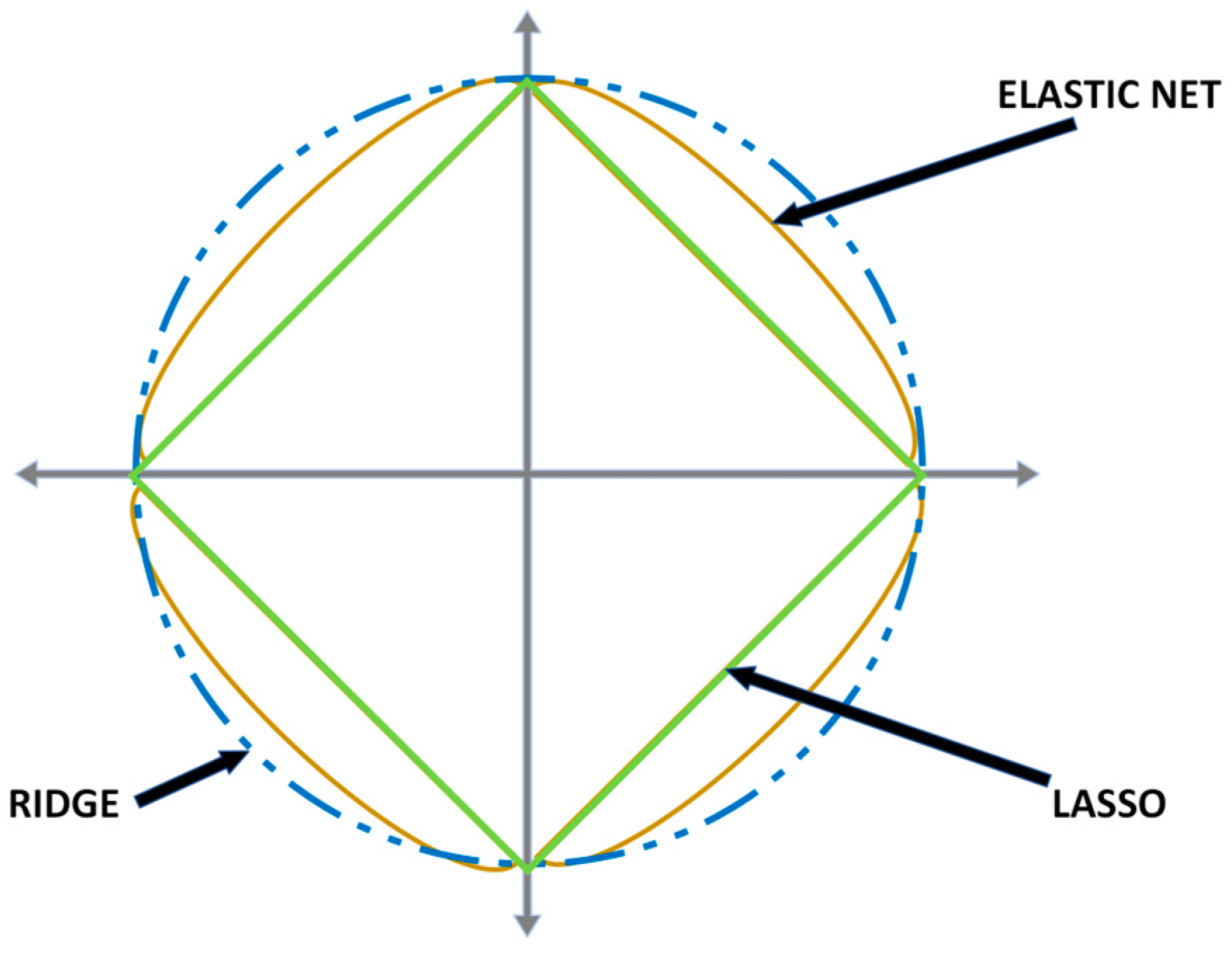
Another model developed within the scope of this study was Elastic Net. It is a regression method that can be used to estimate the discharge capacity of LIBs. Elastic Net combines L1 (Lasso) and L2 (Ridge) regularization terms and, thus, can both perform variable selection and control overfitting. Within the scope of this study, “alpha = 1” was chosen. In this case, Elastic Net uses only L1 regularization. This situation is equivalent to Lasso regression. Additionally, ‘l1_ratio = 1’ was set, and only L1 regularization (Lasso regression) was set to be effective. ‘random_state’ was set to 42, similar to XGBoost.

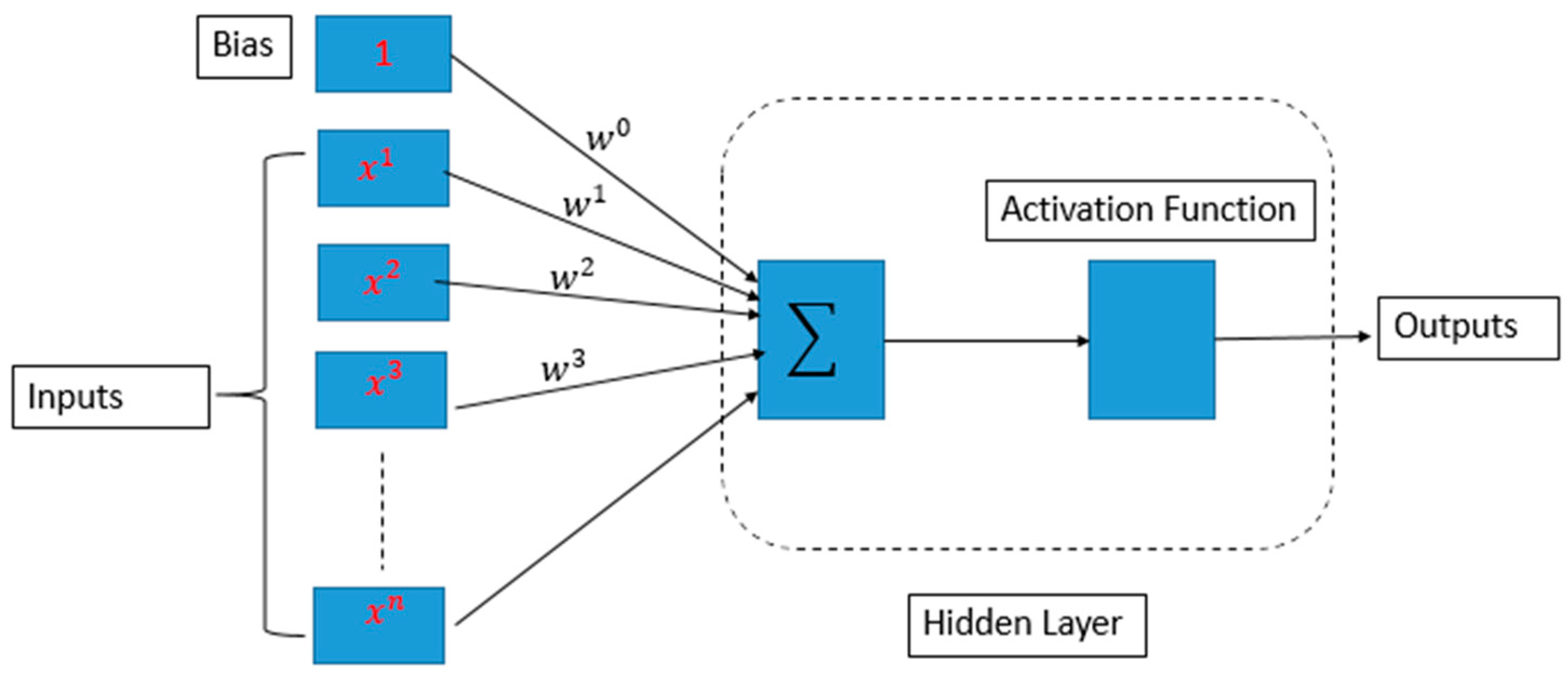
Another model developed within the scope of this study was an MLP, which is a type of deep learning and artificial neural network model. There may be complex and non-linear relationships between factors affecting the LIB capacity. An MLP has the capacity to capture such non-linear relationships and can model complexities.

Table 3. MLP model hyperparameters.

Name of Parameter	Value
hidden_layer_sizes	100, 50
activation	Relu
learning_rate	0.001
batch_size	min (200, n_samples)
random_state	42

shows the hyperparameters used when developing the MLP model.

As stated in Table 3, the first hidden layer had 100 neurons. This layer is used to process input data. The second hidden layer has 50 neurons. This layer receives and processes the outputs from the first hidden layer. The output of the second layer is often used to produce the outputs of the last layer. This means that an MLP has a structure with one or two hidden layers, and these hidden layers contain 100 and 50 neurons, respectively. Additionally, Relu, which is more computationally efficient than some other activation functions, was used. Relu has a non-zero derivative value on positive inputs. This reduces the problem of gradients disappearing during training. The MLP structure’s final layer would typically have a single neuron for regression tasks, outputting the continuous value prediction. The Relu activation function mentioned applies only to hidden layers; often, the output layer in a regression setup would have no activation function (i.e., it is a linear neuron).

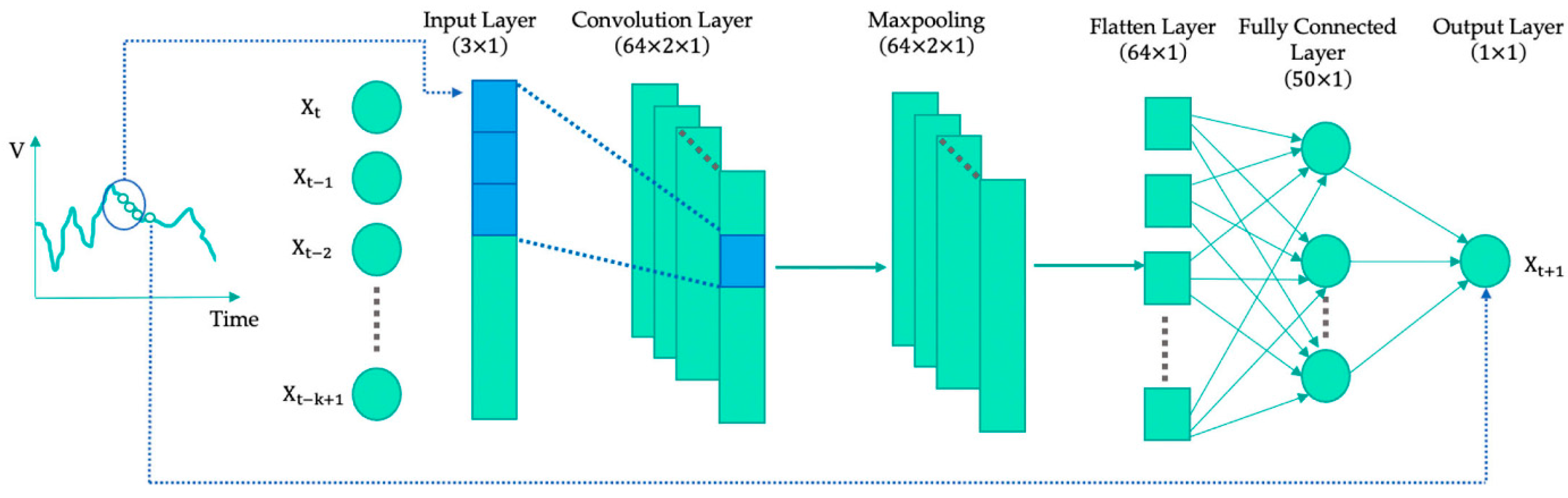
In examining the developed models, it can be considered that the MLP is a subset of deep learning models in the process experienced from an RF to an MLP. An MLP is known as a neural network consisting of an input layer, one or more hidden layers, and output layers. Deep learning models, on the other hand, refer to neural networks containing more layers. These models can consist of much deeper networks (tens or hundreds of layers). MLPs are simpler models that handle smaller datasets and require less computing power. However, deep learning models are more complex and larger models that require larger datasets and higher computing power. Therefore, their success is higher. The first deep learning model developed within the scope of this study is CNN-based. The hyperparameters used in the developed CNN model are presented in

Table 4. CNN model hyperparameters.

Name of Parameter	Value
Convolution layer filters	64
Convolution layer kernel size	3
Activation function of the convolution layer	Relu
Convolution layer padding	same
Pooling layer pool size	2
Pooling layer padding	Same
Batch size	16
Learning rate	0.001
Optimizer	Adam
Loss function	Mean_squared_error
Number of Epochs	100

.

The convolution layer filters parameter determines the depth of the amount of information that the model can learn. Generally, a larger value of the state size allows more complex features to be learned. However, it also increases the risk of overfitting. Therefore, it must be determined according to the amount of data. The hyperparameters specified for the CNN model in Table 4 were judiciously chosen to strike a balance between model complexity and computational efficiency while ensuring effective learning. Utilizing 64 filters in the convolution layer with a kernel size of three and ‘same’ padding enables the extraction of meaningful features without losing spatial dimensions. In order to increase the calculation efficiency and generalization ability of the model, the batch size value was determined to be 16. ‘Relu’ was used as the activation function in the model. The MSE was chosen as the loss function of the model. The MSE is a metric commonly used in regression tasks that takes the average square of the difference between predicted values and actual values. After the parameters were determined, the model was trained for 100 epochs. In this way, it was aimed for the model to achieve sufficient learning from the training dataset and at the same time avoid the risk of overfitting. Each of these parameters was carefully selected to optimize both the performance and generalization of the model. After the completion of the CNN training, a different deep learning model, the RNN model, was developed within the scope of this study. 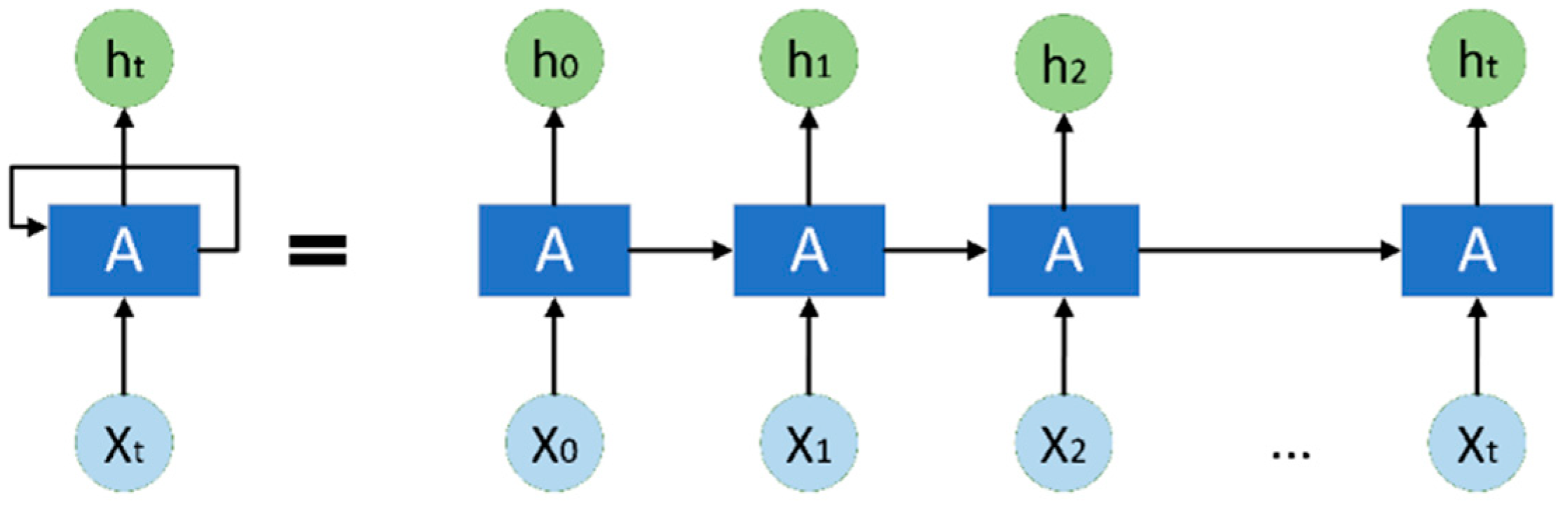Similar hyperparameters to those listed in Table 3 were used in the development of the RNN, which was designed to process sequential data and temporal dependencies. Thus, preparations were made for comparing experimental results and interpreting them on similar infrastructures.

The time dependencies for the RNN developed in this study are related to its ability to process sequential data and temporal dependencies. Unlike feed-forward neural networks, RNNs have a memory that captures information about what has been calculated so far, integrating past information to the current task. This memory is crucial for tasks involving sequences, where the context and the order of elements are important for understanding or prediction. In the context of estimating the discharge capacity of LIBs, the RNN model would leverage its capacity to process sequential data to model how the battery’s discharge capacity changes over time. This involves analyzing time series data of battery usage, including charge/discharge cycles at various C-rates and temperatures, to predict the future capacity or identify patterns indicating battery health.

4. Results

Several studies have been conducted for years on the development of better material compositions for LIBs, their maintenance, and the improvement of their cycle life. In addition to all these parameters, the accurate estimation of the SoH in battery management systems where these batteries are used is essential as it significantly affects the performance of the systems. Especially with the increasing interest in electric vehicles, the tendency to study SoH prediction for LIBs has increased. Therefore, determining the SoH is of great importance. However, due to SoH determination, which is an output of a chemical reaction series that occurs in the LIB during cycles, there is still no consensus of how it can be defined. Thus, following various approaches using statistical methods appears to be the best way at the moment.

4.1. Evaluation Metrics

More than one method was utilized to test the models prepared within the scope of this study. The RMSE, a metric employed to evaluate the accuracy of statistical predictions, was used in the initial testing processes [33]. The RMSE is calculated as the square root of the mean square of the differences between the predicted values and the actual values (Equation (2)):

$$RMSE=\sqrt{\sum _{i=1}^n\frac{{({\hat{a}}_i-a_i)}^2}{n}}$$

(2)

When the RMSE is used to test a developed model, the RMSE is expected to be low. A high RMSE means that the predictions are very different from the actual values. This situation shows a low performance of the model. A lower RMSE value indicates that the predictions are closer to the actual values, and therefore, the model performs better. Additionally, MSE results are also provided, which penalize larger errors more.

Another approach used for model testing in experimental studies is the MAE [34]. Often used to measure the performances of regression models, the MAE represents the mean absolute difference between predicted values and actual values. In other words, it tries to determine how ‘wrong’ each prediction is. The MAE is calculated as expressed in Equation (3):

$$MAE=\left(1/n\right)\sum _{i=1}^n|y_i-{\widehat{y}}_i|$$

(3)

For each prediction, the difference between the predicted value and the actual value is calculated, as shown in Equation (3). Then, the absolute value of this difference is taken. Here, $n$ represents the number of data points. While $y_i$ refers to the true value (observation), ${\widehat{y}}_i$, refers to the value predicted by the model. Essentially, the MAE measures the magnitude of forecast errors and treats each error with the same weight. Additionally, the R-squared error was used as an evaluation metric in this study. The R-squared error measures the explanatory power of the model on the data and expresses how much of the variance of the dependent variable it explains. For this reason, it was used within the scope of the study to measure the effect of independent variables on the dependent variable and to evaluate the explanatory ability of the model. In addition, it is known that the MSE and RMSE metrics do not cover the forecast trend in the time series. For this reason, Prediction of Change in Direction (POCID) was used in this study, which solves the problem by counting the number of correct direction changes [35]. The POCID is a percentage measure calculated as in Equations (4) and (5):

$$POCID=\frac{1}{N-1}\sum _{t=1}^{N-1}D\left(t\right)\cdot 100$$

(4)

$$D\left(t\right)=\left\{\begin{array}{l}1, if \left(Y\left(t+1\right)-Y\left(t\right)\right)\left(\widehat{Y}\left(t+1\right)-\widehat{Y}\left(t\right)\right)>0\\ 0, otherwise \end{array}\right.$$

(5)

4.2. Estimation of Discharge Capacities with Tree and Regression-Based Approaches

XGBoost and RF are two different models, both of which are considered ensemble learning methods and are employed to solve machine learning tasks such as classification and regression. XGBoost aims to create a strong model by combining weak learning models (usually decision trees) with gradient boosting. XGBoost can be thought of as a library that develops and optimizes the gradient boosting method. RF, on the other hand, collects the results by bringing together many decision trees. Each tree is constructed using a random subset of features. XGBoost splits trees by sorting them with a certain feature. This allows for better trees to be created. The success rates of the RF and XGBoost models developed within the scope of this study are presented in

Table 5. Performance comparison of RF and XGBoost models.

Model	MSE	R-Squared	RMSE	MAE	POCID
RF	0.022	0.877	0.148	0.099	83.38
XGBoost	0.026	0.853	0.162	0.110	83.31

. Discharge capacity estimations were calculated using the different models; accordingly, RF seems to be the best estimation method compared with XGBoost.

In examining Table 5, RF achieved better results. It is desirable for the MSE to be low, and a good regression model should have low MSE values. However, the absolute value of MSE alone is not always sufficient for evaluating the quality of a model. Therefore, it should be evaluated together with other metrics. In the examinations, the low R-squared value of RF means that the model can explain only a small part of the variance of the independent variables on the dependent variable. This indicates that the model has weak explanatory power. The RMSE, on the other hand, always depends on the problem and data context. The datasets used in these experiments may have higher RMSE values because the dataset inherently had more variance. Therefore, data characteristics and problem requirements should be taken into consideration while interpreting the RMSE value. Based on this information, it can be predicted that XGBoost can achieve better results when there are more dependent variables. However, preliminary results showed that RF achieved better results. Figure 8 illustrates the actual values produced by the RF and XGBoost models and the distribution of the predicted values.

Within the scope of this study, a different approach that could be used in the regression analysis, such as that of XGBoost and RF, was included in the experiments. Elastic Net is a regression method and is used specifically for linear regression problems. While Elastic Net is used for basic regression analyses and variable selection, XGBoost is preferred for more complex and high-performance classification and regression tasks. Therefore, the Elastic Net model was also developed in this study. The Elastic Net model’s results are included with the performance comparison of the RF and XGBoost models in

Table 6. Performance comparison of RF, XGBoost, and Elastic Net models.

Model	MSE	R-Squared	RMSE	MAE	POCID
RF	0.022	0.877	0.148	0.099	83.38
XGBoost	0.026	0.853	0.162	0.110	83.31
Elastic Net	0.136	0.243	0.369	0.217	72.25

.

Different machine learning algorithms such as Elastic Net, XGBoost, and RF have different structures and capabilities. Elastic Net creates a linear regression model. This means a model of lower complexity that can express simpler relationships. Figure 9 demonstrates the actual values produced by Elastic Net and the distribution of the predicted values.

4.3. Estimation of Discharge Capacity with Deep Learning-Based Algorithms

Although Elastic Net and other machine learning approaches provide successful results, they did not achieve the desired level of success. Therefore, deep learning-based models were developed within the scope of this study. First of all, a simple MLP model belonging to the field of deep learning was developed. Then, CNN and RNN models were used, and comparative results were obtained.

Table 7. Performance comparison of deep learning-based models.

Model	MSE	R-Squared	RMSE	MAE	POCID
MLP	0.059	0.670	0.243	0.135	80.74
RNN	0.046	0.743	0.213	0.127	83.19
CNN	0.042	0.761	0.207	0.124	81.70

shows the results of the deep learning models.

The MLP, RNN, and CNN models in Table 7 are different neural network architectures, and each has advantages and disadvantages. The MLP works specifically with flat feature vectors that do not contain a structural pattern or sequential data. That is, its ability to recognize a structural pattern or infer features in sequential data is limited. The CNN and RNN can better handle structured and sequential data, such as visual or textual data. Hence, the changing conditions of LIBs over time were better captured. Moreover, with the RNN, LSTM and GRU models were employed in line with the desire to make better use of historical data. In addition to the RNN and CNN models used, two LSTM layers of 64 and 48 units, respectively, both using ‘tanh’ activation, were included in the developed models. Likewise, two GRU layers of 64 and 48 units, respectively, were included. However, the ‘Relu’ activation function was chosen for the GRU. Experimental studies have shown that LSTM and GRU models provide similar results. Nevertheless, considering that hybrid models will yield more successful results, hybrid structures of RNN and CNN models with LSTM and GRU models were developed in this study. Performance comparisons of the hybrid structures are presented in

Table 8. Performance comparison of deep learning-based hybrid models.

Model	MSE	R-Squared	RMSE	MAE	POCID
RNN + LSTM	0.043	0.758	0.208	0.124	83.24
RNN + GRU	0.040	0.774	0.201	0.121	83.17
CNN + LSTM	0.039	0.782	0.197	0.122	82.81
CNN + GRU	0.039	0.779	0.199	0.122	83.04

.

In examining Table 8, it is seen that the hybrid models achieved better results than the basic models. A decrease in the MSE indicates that the model has a better fit and its predictions are closer to the actual data. However, the R-Squared value increased slightly. High R-Squared values suggest that the models, particularly those combining an RNN with LSTM or a GRU and CNN with LSTM or a GRU, effectively capture the underlying patterns in the data, leading to accurate predictions. This provided a better explanation of the comparative results. The results obtained highlight our efforts to predict the discharge capacities of LIBs using different models, from simple to complex.

5. Discussion

In this study, we examined the challenges that predictive models, which play a critical role in monitoring the discharge capacity of LIBs, face as they grapple with the evolving technology landscape and increasing complexity. To address the symmetry in battery degradation and charging patterns, we also explored the advantages that deep learning-based models can offer in overcoming these challenges, particularly focusing on how these models can exploit symmetry to enhance predictive accuracy. We also explored the advantages that deep learning-based models can offer in overcoming these challenges and highlighted the importance of these benefits. The advantages of the technology, which emerge through the use of advanced prediction models, make LIBs more efficient and adaptable in terms of battery management and scalability.

Unlike traditional machine learning methods, tree-based and deep learning-based, complex and comprehensive models offer more dynamic structures that can increase the operational efficiency. However, the integration of deep learning-based Li-ion discharge capacity prediction models with contemporary technologies such as decision support systems and big data analytics will increase efficiency and manageability, especially by incorporating symmetry considerations to better mirror the inherent characteristics of battery behavior.

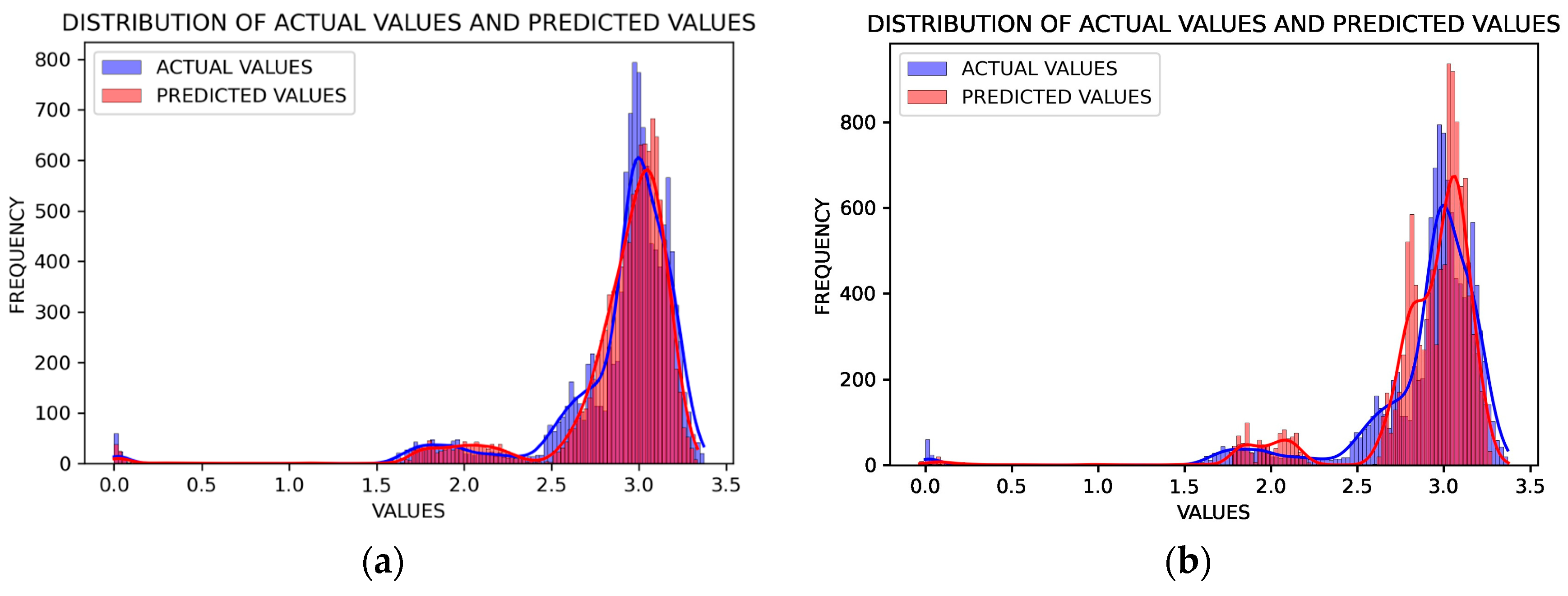
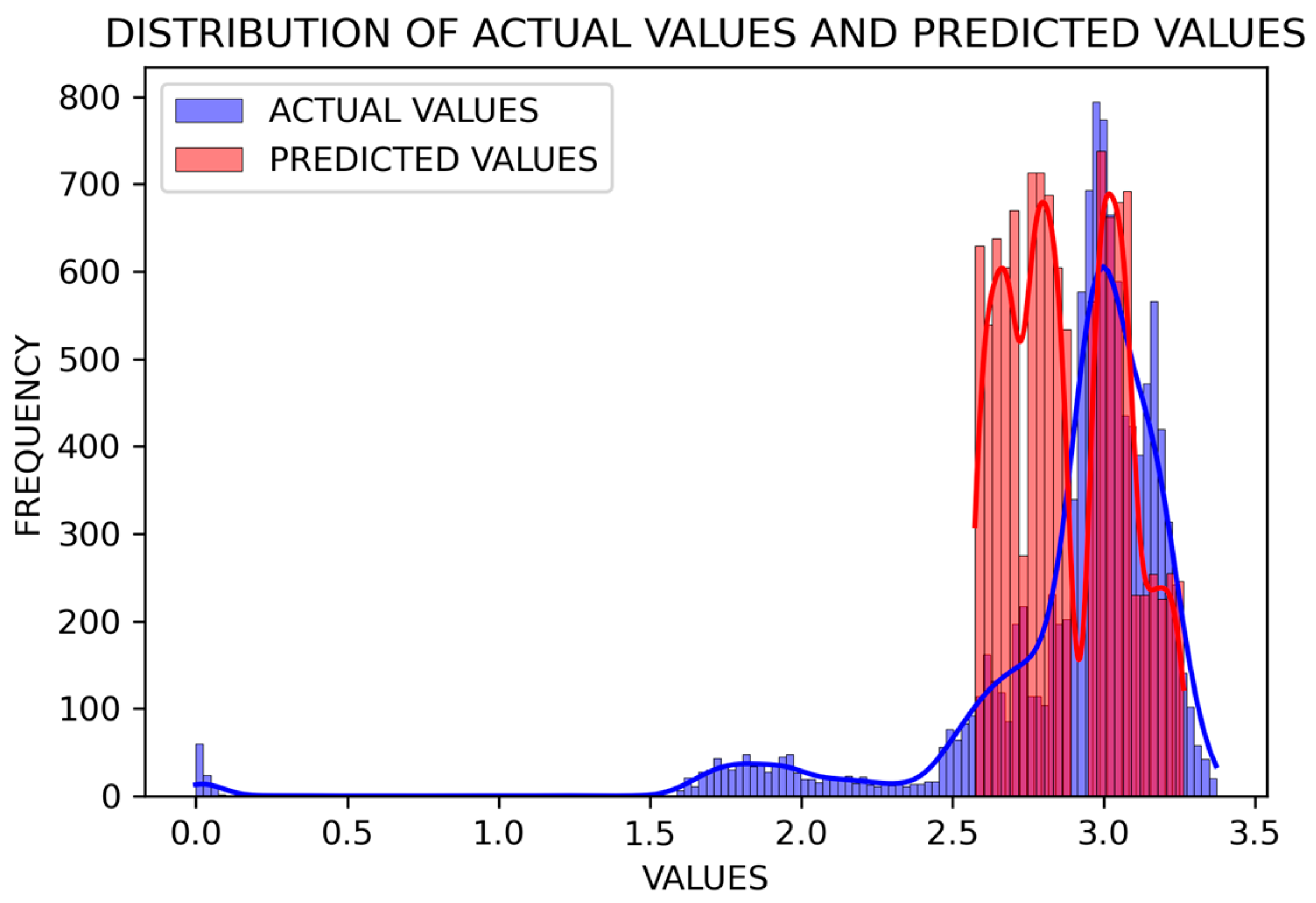
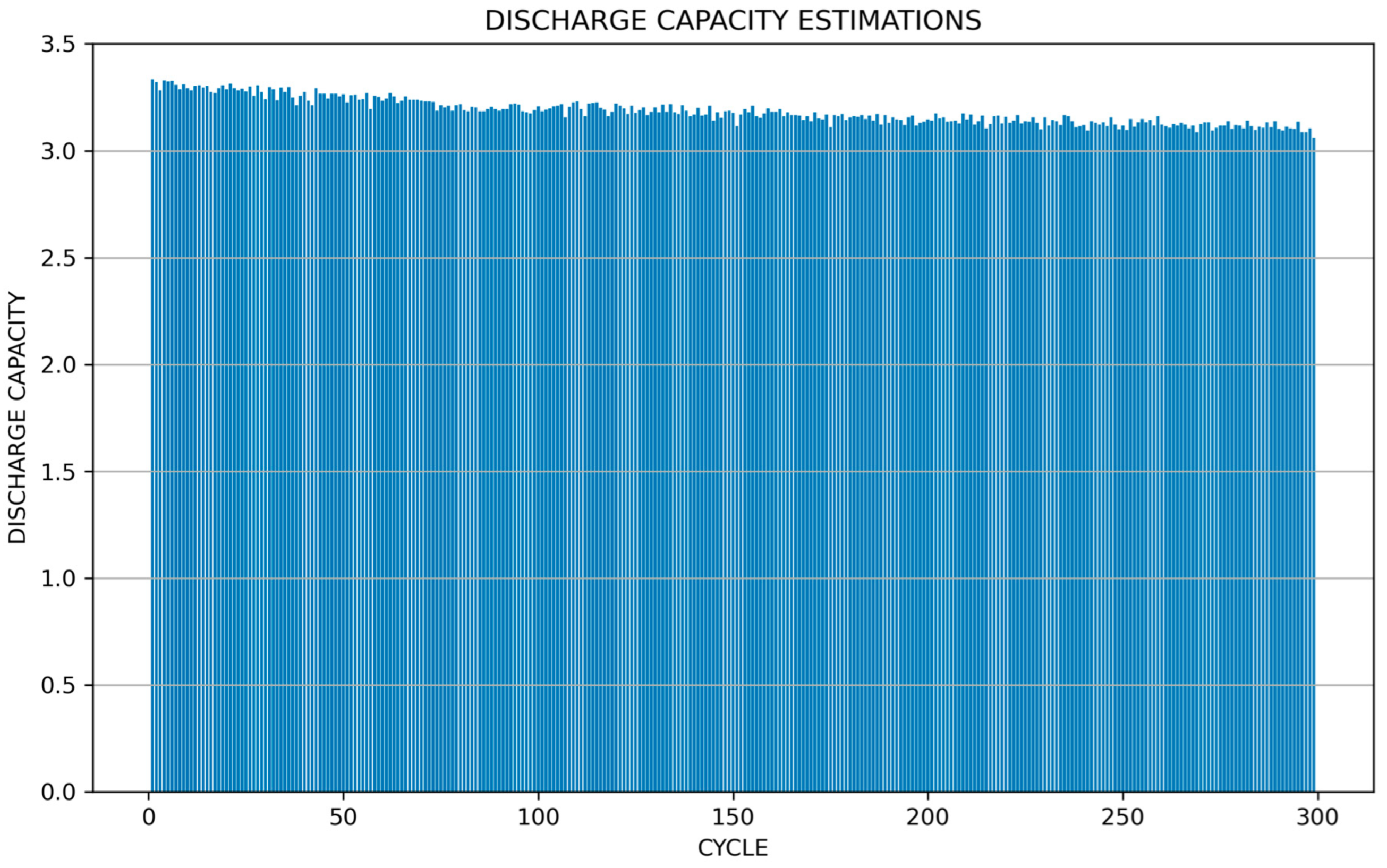
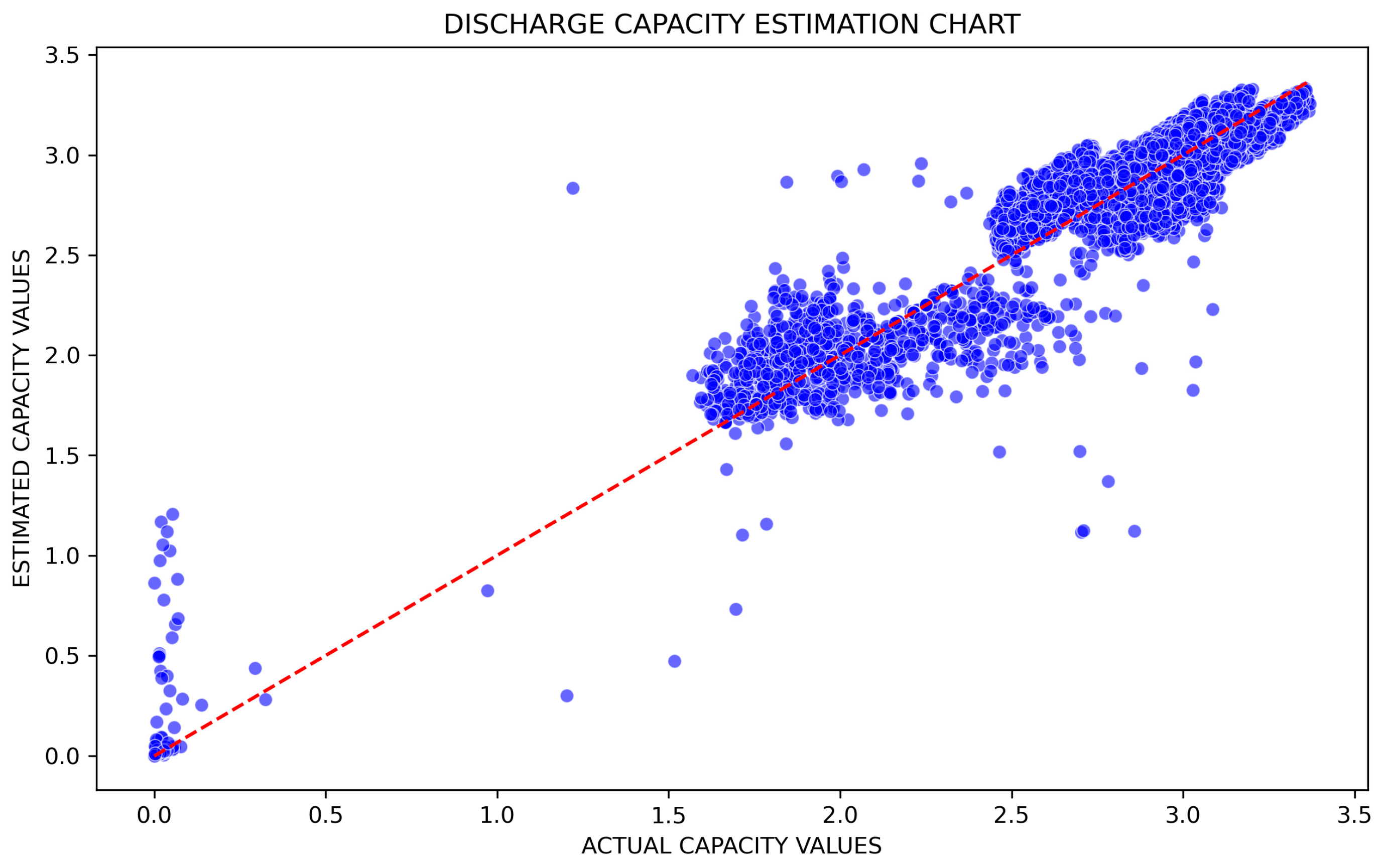
The most important disadvantage of machine learning models is that there is no standard way to determine model parameters. Model parameters were chosen based on default values that are widely accepted. These parameters may vary depending on the dataset and problem used, and similar parameters used as much as possible in order to better evaluate the common results of different models. When the results were examined, it could be seen that RF is the most successful method among the different models created for estimating the discharge capacity of batteries. The fact that the RMSE and MAE values were close to zero and the R-Squared value was close to 1 showed that our proposed model is more successful. In addition, when the POCID and other evaluation criteria were examined, it was seen that the RF model was more successful than other machine learning models and minimized the prediction error. Based on the experiments conducted with the RF machine learning model, an estimation graph is shown in Figure 10, and a discharge capacity estimation graph is shown in Figure 11.

In examining Figure 10, it is seen that the SoH estimation decreases regularly in line with the cycle increase. Figure 11 is presented to better visualize this situation. If the results are considered as part of a regression problem, it can be said that the results obtained provide important information about discharge capacities. The experiments carried out in this study were compared with complex processes from many studies. So, in order to demonstrate understandability within the scope of this study, the experiments were carried out on many models, from basic machine learning approaches to hybrid deep learning approaches. The strategic use of various evaluation metrics notably improved the explainability of our findings, making the sophisticated processes more accessible and comprehensible. This comprehensive evaluation approach ensures that complex modeling processes are broken down into more understandable parts, facilitating clearer insights into how the model performs under different conditions.

We proposed a decision support system designed for the prediction of discharge capacities through the application of an RF-based model approach. This approach achieved the best results on the dataset used in this study. The integration of factors such as feature selection, the development of different models, and hyperparameter settings contributed to improving the efficiency of LIBs. The findings of this study will make a valuable contribution to the development of efficient and high-performance battery technologies in the energy sector by further advancing the integration of LIB technology into future decision support systems and electronic devices that use batteries. There are many articles published in the literature on solving the problem of estimating discharge capacities. In these studies, test data containing different temperatures and charge and discharge currents are generally used to estimate the discharge capacities of LIBs from traditional machine learning and hybrid models. Considering these data, machine learning-based prediction methods such as SVM, KNN, RF, and MLP are frequently used for prediction algorithms and models.

Table 9. Performance comparison of models from previous studies in the literature.

Ref.	Datasets	ML Algorithms	R-Squared	RMSE	MAE
[36]	Oxford Dataset	SVR	0.89	1.11	-
[37]	Oxford Dataset	LSTM	0.98	0.06	-
[38]	Shu et al. (2022)	RF	-	0.54	1.63
[39]	Wang et al. (2021)	RF	0.59	-	-
[40]	Hannan et al. (2021)	LSTM	-	1.69	0.54
[40]	Hannan et al. (2021)	DNN	-	11.05	8.64

shows a comparison of the proposed model with those of previous studies. However, the data, methods, and success rates obtained vary from study to study.

The comparative performance analyses as shown in Table 7, Table 8 and Table 9 show that the MLP, RNN, and CNN models have different degrees of effectiveness in comparison to the benchmark literature values as measured using the R-squared, RMSE and MAE metrics. In particular, the hybrid deep learning models RNN + LSTM, RNN + GRU, CNN + LSTM, and CNN + GRU outperform their counterparts and the cited literature models. The improved performances of these hybrid models are attributed to their superior handling of the complexities inherent in the dataset used in this study, showcasing their robustness in modeling and prediction tasks.

6. Conclusions and Future Trends

This study presented an end-to-end model research on predicting the discharge capacity of LIBs and achieved significant results. Our research started with collecting original data and applying data pre-processing steps, followed by conducting a series of experiments to evaluate the performances of various machine learning algorithms and deep learning models.

The results obtained show that this study, when using original data, could develop powerful models that can successfully predict the discharge capacity of LIBs. Traditional machine learning algorithms such as RF, XGBoost, and MLP yielded valuable results in terms of prediction performance. In addition, hybrid models developed with deep learning-based CNN and RNN architectures demonstrated high performances on time series data, and their performance effects became more explainable when analyzed within the scope of the concept of symmetry. Hybrid models developed with deep learning-based CNN and RNN architectures demonstrated high performance on time series data. The performances of hybrid models such as CNN-LSTM, CNN-GRU, RNN-LSTM, and RNN-GRU highlighted the power of deep learning approaches in time series forecasting. On the other hand, the first values obtained showed that RF-based models achieved more successful results.

This study offers important insights for guiding future researchers in estimating the discharge capacity of LIBs, which are an important component of energy storage technologies. This study shows that deep learning models have great potential in LIB capacity prediction. Future works might focus on further improving and extending deep learning methods. LIBs are used under many different models and operating conditions. Future research might contribute to better establishing generalizations by considering different battery models and environmental conditions, with a particular focus on symmetrical behaviors. Collecting more data and improving data pre-processing methods can improve model performances. Future works might also focus more on choosing optimal models and algorithms for specific applications. Techniques such as automatic model selection and hyperparameter tuning may help researchers.

This research laid the foundation for future innovations and developments in the field of LIBs and energy storage systems and contributes to researchers making further progress in this field. Future studies may build on this foundation to achieve further achievements and contributions in this field.

References

1. Liu, D.; Song, Y.; Li, L.; Liao, H.; Peng, Y. On-line life cycle health assessment for lithium-ion battery in electric vehicles. J. Clean. Prod. 2018, 199, 1050–1065. [Google Scholar] [CrossRef]
2. Gan, L.; Yang, F.; Shi, Y.F.; He, H.L. Lithium-ion battery state of function estimation based on fuzzy logic algorithm with associated variables. IOP Conf. Ser. Earth Environ. Sci. 2017, 94, 012133. [Google Scholar] [CrossRef]
3. Yao, H.; Jia, X.; Zhao, Q.; Cheng, Z.-J.; Guo, B. Novel Lithium-Ion Battery State-of-Health Estimation Method Using a Genetic Programming Model. IEEE Access 2020, 8, 95333–95344. [Google Scholar] [CrossRef]
4. Song, Y.; Liu, D.; Liao, H.; Peng, Y. A hybrid statistical data-driven method for on-line joint state estimation of lithium-ion batteries. Appl. Energy 2020, 261, 114408. [Google Scholar] [CrossRef]
5. Zhai, Q.; Ye, Z.-S. RUL Prediction of Deteriorating Products Using an Adaptive Wiener Process Model. IEEE Trans. Ind. Inform. 2017, 13, 2911–2921. [Google Scholar] [CrossRef]
6. Cai, L.; Meng, J.; Stroe, D.-I.; Peng, J.; Luo, G.; Teodorescu, R. Multiobjective Optimization of Data-Driven Model for Lithium-Ion Battery SOH Estimation with Short-Term Feature. IEEE Trans. Power Electron. 2020, 35, 11855–11864. [Google Scholar] [CrossRef]
7. Xue, Z.; Zhang, Y.; Cheng, C.; Ma, G. Remaining useful life prediction of lithium-ion batteries with adaptive unscented kalman filter and optimized support vector regression. Neurocomputing 2019, 376, 95–102. [Google Scholar] [CrossRef]
8. Özden, S.; Dursun, M.; Aksöz, A.; Saygın, A. Prediction and modelling of energy consumption on temperature control for greenhouses. J. Polytech. 2018, 22, 213–217. [Google Scholar] [CrossRef]
9. Liu, Y.; Zhao, G.; Peng, X. Deep learning prognostics for lithium-ion battery based on ensembled long short-term memory networks. IEEE Access 2019, 7, 155130–155142. [Google Scholar] [CrossRef]
10. Liu, K.; Shang, Y.; Ouyang, Q.; Widanage, W.D. A Data-Driven Approach with Uncertainty Quantification for Predicting Future Capacities and Remaining Useful Life of Lithium-ion Battery. IEEE Trans. Ind. Electron. 2021, 68, 3170–3180. [Google Scholar] [CrossRef]
11. Alhamayani, A. CNN-LSTM to Predict and Investigate the Performance of a Thermal/Photovoltaic System Cooled by Nanofluid (Al2O3) in a Hot-Climate Location. Processes 2023, 11, 2731. [Google Scholar] [CrossRef]
12. Toughzaoui, Y.; Toosi, S.B.; Chaoui, H.; Louahlia, H.; Petrone, R.; Le Masson, S.; Gualous, H. State of health estimation and remaining useful life assessment of lithium-ion batteries: A comparative study. J. Energy Storage 2022, 51, 104520. [Google Scholar] [CrossRef]
13. Oyucu, S.; Doğan, F.; Aksöz, A.; Biçer, E. Comparative Analysis of Commonly Used Machine Learning Approaches for Li-Ion Battery Performance Prediction and Management in Electric Vehicles. Appl. Sci. 2024, 14, 2306. [Google Scholar] [CrossRef]
14. Sekulić, A.; Kilibarda, M.; Heuvelink, G.B.; Nikolić, M.; Bajat, B. Random Forest spatial interpolation. Remote. Sens. 2020, 12, 1687. [Google Scholar] [CrossRef]
15. Chen, T.; He, T.; Benesty, M. XGBoost: eXtreme Gradient Boosting. R Packag. 2018, Comprehensive r archive network. version 0.71-2, 1–4.
16. De Mol, C.; De Vito, E.; Rosasco, L. Elastic-net regularization in learning theory. J. Complex. 2009, 25, 201–230. [Google Scholar] [CrossRef]
17. Khalid, A.; Sundararajan, A.; Acharya, I.; Sarwat, A.I. Prediction of Li-Ion Battery State of Charge Using Multilayer Perceptron and Long Short-Term Memory Models. In Proceedings of the 2019 IEEE Transportation Electrification Conference and Expo (ITEC), Detroit, MI, USA, 19–21 June 2019; IEEE: Piscataway, NJ, USA, 2019; pp. 1–6. [Google Scholar] [CrossRef]
18. Song, Y.; Li, L.; Peng, Y.; Liu, D. Lithium-Ion Battery Remaining Useful Life Prediction Based on GRU-RNN. In Proceedings of the 2018 12th International Conference on Reliability, Maintainability, and Safety (ICRMS), Shanghai, China, 17–19 October 2018; Volume 61771157, pp. 317–322. [Google Scholar] [CrossRef]
19. Chicco, D.; Warrens, M.J.; Jurman, G. The coefficient of determination R-squared is more informative than SMAPE, MAE, MAPE, MSE and RMSE in regression analysis evaluation. PeerJ Comput. Sci. 2021, 7, e623. [Google Scholar] [CrossRef]
20. Diao, W.; Saxena, S.; Pecht, M. Accelerated cycle life testing and capacity degradation modeling of LiCoO2-graphite cells. J. Power Sources 2019, 435, 226830. [Google Scholar] [CrossRef]
21. Radivojević, D.S.; Lazović, I.M.; Mirkov, N.S.; Ramadani, U.R.; Nikezić, D.P. A Comparative Evaluation of Self-Attention Mechanism with ConvLSTM Model for Global Aerosol Time Series Forecasting. Mathematics 2023, 11, 1744. [Google Scholar] [CrossRef]
22. Jin, Z.; Shang, J.; Zhu, Q.; Ling, C.; Xie, W.; Qiang, B. RFRSF: Employee Turnover Prediction Based on Random Forests and Survival Analysis. Lect. Notes Comput. Sci. 2020, 12343, 503–515. [Google Scholar] [CrossRef]
23. Yan, N.; Yao, Y.-B.; Jia, Z.-D.; Liu, L.; Dai, C.-T.; Li, Z.-G.; Zhang, Z.-H.; Li, W.; Wang, L.; Wang, P.-F. Online battery health diagnosis for electric vehicles based on DTW-XGBoost. Energy Rep. 2022, 8, 121–128. [Google Scholar] [CrossRef]
24. Wei, D.S. Strong Approximation for a Toric Variety. Acta Math. Sin. Engl. Ser. 2021, 37, 95–103. [Google Scholar] [CrossRef]
25. Noriega, L. Multilayer Perceptron Tutorial. 2005. Available online: https://api.semanticscholar.org/CorpusID:61645526 (accessed on 27 March 2024).
26. Han, Y.; Li, C.; Zheng, L.; Lei, G.; Li, L. Remaining Useful Life Prediction of Lithium-Ion Batteries by Using a Denoising Transformer-Based Neural Network. Energies 2023, 16, 6328. [Google Scholar] [CrossRef]
27. Sumayli, A. Development of advanced machine learning models for optimization of methyl ester biofuel production from papaya oil: Gaussian process regression (GPR), multilayer perceptron (MLP), and K-nearest neighbor (KNN) regression models. Arab. J. Chem. 2023, 16, 104833. [Google Scholar] [CrossRef]
28. Rahimi, A.; Gönen, M. Discriminating early- and late-stage cancers using multiple kernel learning on gene sets. Bioinformatics 2018, 34, i412–i421. [Google Scholar] [CrossRef] [PubMed]
29. Camacho Olmedo, M.T.; Paegelow, M.; Mas, J.F.; Escobar, F. Geomatic Approaches for Modeling Land Change Scenarios; Part of the Lecture Notes in Geoinformation and Cartography Book Series (LNGC); Springer International Publishing: New York, NY, USA, 2018; pp. 1–8. [Google Scholar] [CrossRef]
30. Duman, E.; Erdem, O.A. Anomaly Detection in Videos Using Optical Flow and Convolutional Autoencoder. IEEE Access 2019, 7, 183914–183923. [Google Scholar] [CrossRef]
31. He, K.; Yang, Q.; Ji, L.; Pan, J.; Zou, Y. Financial Time Series Forecasting with the Deep Learning Ensemble Model. Mathematics 2023, 11, 1054. [Google Scholar] [CrossRef]
32. Rincón-Maya, C.; Guevara-Carazas, F.; Hernández-Barajas, F.; Patino-Rodriguez, C.; Usuga-Manco, O. Remaining Useful Life Prediction of Lithium-Ion Battery Using ICC-CNN-LSTM Methodology. Energies 2023, 16, 7081. [Google Scholar] [CrossRef]
33. Srinivasan, A.R.; Lin, Y.-S.; Antonello, M.; Knittel, A.; Hasan, M.; Hawasly, M.; Redford, J.; Ramamoorthy, S.; Leonetti, M.; Billington, J.; et al. Beyond RMSE: Do Machine-Learned Models of Road User Interaction Produce Human-Like Behavior? IEEE Trans. Intell. Transp. Syst. 2023, 24, 7166–7177. [Google Scholar] [CrossRef]
34. Khair, U.; Fahmi, H.; Al Hakim, S.; Rahim, R. Forecasting Error Calculation with Mean Absolute Deviation and Mean Absolute Percentage Error. J. Phys. Conf. Ser. 2017, 930, 012002. [Google Scholar] [CrossRef]
35. Cocianu, C.L.; Uscatu, C.R.; Avramescu, M. Improvement of LSTM-Based Forecasting with NARX Model through Use of an Evolutionary Algorithm. Electronics 2022, 11, 2935. [Google Scholar] [CrossRef]
36. Lin, M.; Yan, C.; Meng, J.; Wang, W.; Wu, J. Lithium-ion batteries health prognosis via differential thermal capacity with simulated annealing and support vector regression. Energy 2022, 250, 123829. [Google Scholar] [CrossRef]
37. Lim, L.D.; Tan, A.F.J.; Tomacruz, J.G.T.; Castro, M.T.; Remolona, M.F.M.; Ocon, J.D. Cyclic Degradation Prediction of Lithium-Ion Batteries using Data-Driven Machine Learning. Chem. Eng. Trans. 2022, 94, 787–792. [Google Scholar] [CrossRef]
38. Shu, X.; Shen, J.; Chen, Z.; Zhang, Y.; Liu, Y.; Lin, Y. Remaining capacity estimation for lithium-ion batteries via co-operation of multi-machine learning algorithms. Reliab. Eng. Syst. Saf. 2022, 228, 108821. [Google Scholar] [CrossRef]
39. Wang, G.; Fearn, T.; Wang, T.; Choy, K.-L. Machine-Learning Approach for Predicting the Discharging Capacities of Doped Lithium Nickel–Cobalt–Manganese Cathode Materials in Li-Ion Batteries. ACS Central Sci. 2021, 7, 1551–1560. [Google Scholar] [CrossRef]
40. Hannan, M.A.; How, D.N.T.; Lipu, M.S.H.; Mansor, M.; Ker, P.J.; Dong, Z.Y.; Sahari, K.S.M.; Tiong, S.K.; Muttaqi, K.M.; Mahlia, T.M.I.; et al. Deep learning approach towards accurate state of charge estimation for lithium-ion batteries using self-supervised transformer model. Sci. Rep. 2021, 11, 19541. [Google Scholar] [CrossRef]
Figure 1. Elastic Net vs. Lasso and Ridge estimators.
Symmetry 16 00436 g001
Figure 2. Single layer perceptron.
Symmetry 16 00436 g002
Figure 3. A CNN example [32].
Symmetry 16 00436 g003
Figure 4. RNN internal structure.
Symmetry 16 00436 g004
Figure 5. LSTM architecture [32].
Symmetry 16 00436 g005
Figure 6. GRU basic architecture.
Symmetry 16 00436 g006
Figure 7. Model development and application steps.
Symmetry 16 00436 g007
Figure 8. Distribution of actual values and predicted values produced by RF (a) and XGBoost (b) models.
Symmetry 16 00436 g008
Figure 9. Distribution of actual values and predicted values produced by Elastic Net.
Symmetry 16 00436 g009
Figure 10. Discharge capacity estimation chart.
Symmetry 16 00436 g010
Figure 11. Comparing predicted and actual battery capacity outputs.
Symmetry 16 00436 g011