Direction of Arrival Estimation of Coherent Sources via a Signal Space Deep Convolution Network

Abstract

In the field of direction of arrival (DOA) estimation for coherent sources, subspace-based model-driven methods exhibit increased computational complexity due to the requirement for eigenvalue decomposition. In this paper, we propose a new neural network, i.e., the signal space deep convolution (SSDC) network, which employs the signal space covariance matrix as the input and performs independent two-dimensional convolution operations on the symmetric real and imaginary parts of the input signal space covariance matrix. The proposed SSDC network is designed to address the challenging task of DOA estimation for coherent sources. Furthermore, we leverage the spatial sparsity of the output from the proposed SSDC network to conduct a spectral peak search for obtaining the associated DOAs. Simulations demonstrate that, compared to existing state-of-the-art deep learning-based DOA estimation methods for coherent sources, the proposed SSDC network achieves excellent results in both matching and mismatching scenarios between the training and test sets.

1. Introduction

Direction of arrival (DOA) estimation is a common problem in array signal processing with extensive applications in various domains, including astronomical observations, indoor localization, sonar, radar, wireless communications [1,2,3,4], etc. The principal challenges in DOA estimation encompass the intricate task of devising integrated strategies that exhibit minimal hardware consumption [5] while concurrently optimizing both performance and receiver cost. Additionally, there is a need to enhance the accuracy and super-resolution capabilities of DOA estimation methods in scenarios featuring multiple sources. Moreover, improving the adaptability of DOA estimation techniques in challenging environments characterized by limited snapshots and low signal-to-noise ratios (SNRs) is also a critical area of focus.

Typically, DOA estimation is mostly accomplished using model-driven methods [6,7,8,9,10,11,12,13], where the underlying principle involves constructing a forward parameter model from signal direction to array outputs, followed by leveraging the properties of predefined assumptions to estimate the direction. Subspace-based methods [6,7], as well as compressive sensing and sparse recovery methods, like singular value decomposition (SVD) [8,9], sparse Bayesian learning (SBL) [10,11], and orthogonal matching pursuit (OMP) [12,13], are commonly utilized in DOA estimation. The model-driven techniques depend on the accuracy of the pre-established model, making it challenging to achieve high accuracy under non-ideal conditions, e.g., coherent sources [14] may lead to significant performance degradation of the algorithms mentioned above.

In recent years, machine learning (ML) [15] approaches utilizing data-driven models [16] have been widely adopted by researchers to address the source localization problem. Deep neural network (DNN)-based methods aim to directly learn the nonlinear relationship between array output and source location, facilitating an efficient mapping from the sensor output space to the arrival direction space. The rapid advancement of artificial intelligence has led researchers to incorporate radial basis function (RBF), support vector regression (SVR) [17], and deep learning (DL) [18,19,20,21,22] into DOA estimation, with the goal of enhancing both accuracy and computational efficiency. In [19], a DL framework for DOA estimation is introduced, specifically designed to handle array imperfections effectively. In [20], the authors demonstrate that the columns of array covariance matrix be formulated as undersampled noisy linear measurements of the spatial spectrum and presented a deep convolutional network (DCN) framework for estimating the DOAs. Additionally, in [21], the authors propose a convolutional neural network (CNN) that effectively learns the number of sources and DOAs even in extreme SNR scenarios. Moreover, in [22], a novel DOA estimation method based on dimensional alternating fully-connected (DAFC) block-based neural networks (NNs) is presented, specifically designed to address spatial spectrum estimation in multi-source scenarios where non-Gaussian spatial color interference is present, and the number of sources is unknown a priori. Ref. [23] designs deep augmented (DA)-MUSIC neural architectures to overcome the limitations of traditional algorithms and combines model-/data-driven hybrid DOA estimators to improve the resolution of the signals. Ref. [24] proposes a DNN-based DOA estimation framework for uniform circular array (UCA) to realize more efficient data transmission in high-capacity communication networks. In the field of sound source localization, Ref. [25] proposes new frequency-invariant circular harmonic features as inputs to the network structure, utilizing CNN for self-adaptation to array defects. Nevertheless, the aforementioned methodologies [16,17,18,19,20,21,22,23,24,25] share a common prerequisite for accurate DOA estimation–-these sources are irrelevant. Regarding coherent signals, finding appropriate data characteristics and constructing a more efficient learning model is our motivation.

For coherent sources, model-driven methods for solving the coherent source problem require spatial smoothing (SS) techniques [26,27,28], albeit at the expense of a reduced effective array aperture. On the contrary, data-driven methods are employed to improve the estimation accuracy and realize real-time updates. In [29], two angle separation learning schemes (ASLs) are proposed to solve the coherent DOA estimation issue, taking into consideration the spatial sparsity of the array output regarding angle separation. A logarithmic eigenvalue-based classification network (LogECNet) is introduced in [30] to achieve higher accuracy of signal number detection and angle estimation performance. However, the existing neural network-based methods for addressing coherent sources [29,30] require transforming signal statistics into a long vector input, thereby leading to the requirement for large-sized parameter matrices in the neural layers during the training process.

Existing methods for coherent signal estimation are often hindered by significant computational complexity [26,27,28]. From the above analysis, we propose an effective data-driven method for improving the accuracy and resolution of coherent source estimation. Our main contributions are as follows:

• We propose a novel signal space deep convolution (SSDC) network that learns angular features of coherent signals to address the coherent DOA estimation problem.
• Since the conventional neural network frames are unable to effectively convey information in the complex domain, we divide the covariance matrix of the input signal space into real and imaginary parts and perform two-dimensional convolution operations separately, which can make the features of the input data fully utilized.
• The proposed SSDC network also considers the spatial sparsity of the array output and performs a spectral peak search on the output to determine the interested DOAs.

Notations: Upper-case (lower-case) bold characters represent matrices (vectors). ${\left(·\right)}^T$, ${\left(·\right)}^H$ and ${\left(·\right)}^{†}$ stand for the transpose, hermitian transpose, and pseudo-inverse operations, respectively. $\mathbb{E}\left(·\right)$ denotes the expectation operator, randn is a random number between 0 and 1, and $\mathbb{C}$ represents the set of complex numbers. $real\left(\right)$ and $imag\left(\right)$ represent real and imaginary parts, and j is the imaginary unit, defined as $\sqrt{-1}$.

2. Problem Formulation

2.1. Signal Model

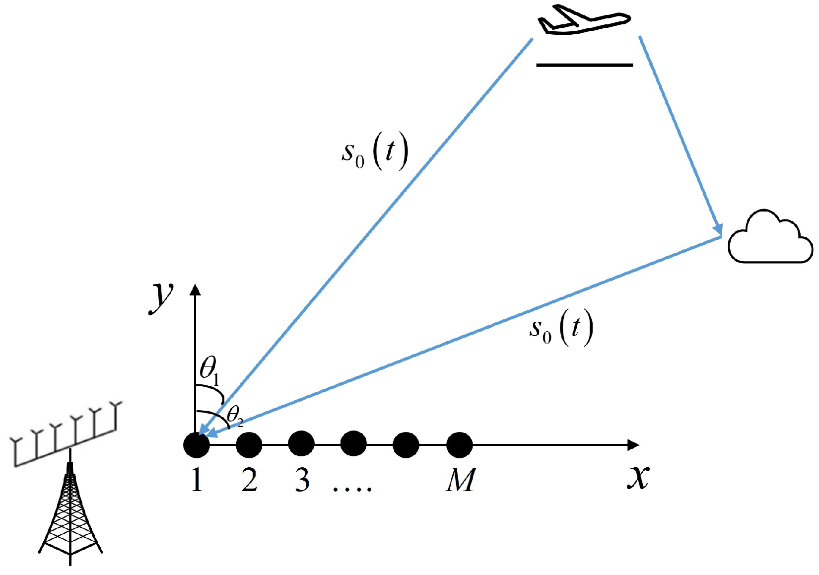
We consider a uniform linear array (ULA) of M-sensors, with space d between two adjacent array sensors, where $d=\frac{\lambda }{2}$ with $\lambda$ being the signal carrier wavelength. As depicted in Figure 1, coherent signals are typically generated from the same signal source or sources with similar properties. We assume that Q narrowband far-field coherent sources ${\theta }_q,q=1,2,\cdots ,Q$ are incident on this ULA. The first sensor is taken as the reference element, as shown in [6]; the data received by all sensors can be represented as

$$\mathbf{z}\left(t\right)=s_0\left(t\right)\sum _{q=1}^Q{\alpha }_q\mathbf{a}\left({\theta }_q\right)+\mathbf{n}\left(t\right)=s_0\left(t\right)\mathbf{A}\mathbf{\alpha }+\mathbf{n}\left(t\right),$$

(1)

where $\mathbf{\alpha }={\left[{\alpha }_1,\cdots ,{\alpha }_q,\cdots ,{\alpha }_Q\right]}^T$ with ${\alpha }_q$ being a nonzero complex-valued constant, $s_0\left(t\right)$ is the direct signal and the reflected one (signal $s_0\left(t\right)={\mu }_0\left(t\right)e^{j{\varphi }_0\left(t\right)}{e}^{j{\omega }_{0}t}$ where ${\mu }_0\left(t\right)$ represents the amplitude and ${\varphi }_0\left(t\right)$ is the phase and $e^{j{\omega }_{0}t}$ is the carrier wave which acts as an information carrier but contains no information). Both the amplitude and phase are statistically independent, and in this paper, we do not consider the variation uncertainty of amplitude and phase of multiple signals, i.e., ${\mu }_0\left(t\right)=1$ and ${\varphi }_0\left(t\right)=0$), $\mathbf{n}\left(t\right)$ represents a circularly symmetric complex additive Gaussian white noise (AWGN), i.e., $\mathbf{n}\left(t\right)\sim \mathcal{C}\mathcal{N}\left(·\left|\mathbf{0},{\sigma }_n^2{\mathbf{I}}_M\right.\right)$ with noise variance ${\sigma }_n^2$, $t=1,\cdots ,T$ and T denotes the number of snapshots. The direction matrix $\mathbf{A}=\left[\mathbf{a}\left({\theta }_1\right),\cdots ,\mathbf{a}\left({\theta }_Q\right)\right]\in {\mathbb{C}}^{M\times Q}$ is defined by

$$\mathbf{a}\left({\theta }_q\right)={\left[1,e^{-j\pi sin{\theta }_q},\cdots ,e^{-j\pi \left(M-1\right)sin{\theta }_q}\right]}^T.$$

(2)

Owing to the spatial properties of the signal parameters, cross-covariance information between different sensors is required, and according to [1], the signal and the noise are statistically independent from each other, so the spatial covariance matrix of Equation (1) can be expressed as

$$\mathbf{R}=\mathbb{E}\left\{\mathbf{z}\left(t\right){\mathbf{z}}^H\left(t\right)\right\}=\mathbf{A}{\mathbf{R}}_s{\mathbf{A}}^H+{\sigma }_n^2{\mathbf{I}}_M,$$

(3)

where ${\mathbf{R}}_s={\sigma }_0^2\mathbf{\alpha }{\mathbf{\alpha }}^H$ is the signal covariance matrix, and ${\sigma }_0^2=\mathbb{E}\left\{{\left|s_0\left(t\right)\right|}^2\right\}$ denotes the reference signal power. Since the incoming sources are fully coherent, ${\mathbf{R}}_s$ is a singular matrix with rank of one. Usually, the covariance matrix can be estimated by the following sample covariance matrix: $\tilde{\mathbf{R}}=1/\phantom{1T}T{\sum }_{t=1}^T\mathbf{z}\left(t\right){\mathbf{z}}^H\left(t\right)$.

As shown in refence [27], by performing eigenvalue decomposition (EVD) of $\mathbf{R}$, we obtain

$$\begin{array}{c}\mathbf{R}=\mathbf{U}\mathbf{\Lambda }{\mathbf{U}}^H={\mathbf{U}}_s{\mathbf{\Lambda }}_s{\mathbf{U}}_s^H+{\mathbf{U}}_N{\mathbf{\Lambda }}_N{\mathbf{U}}_N^H={\displaystyle \sum _{i=1}^M}{\tau }_i{\mathbf{u}}_i{\mathbf{u}}_i^H\hfill \end{array}$$

(4)

where $\mathbf{\Lambda }=diag\left\{{\tau }_1,{\tau }_2,\cdots ,{\tau }_M\right\}$ is a diagonal matrix composed of eigenvalues with ${\tau }_1>{\tau }_2=\cdots {\tau }_Q={\tau }_{Q+1}=\cdots ={\tau }_M={\sigma }_n^2$. The eigenvectors corresponding to eigenvalue ${\tau }_1,\cdots ,{\tau }_M$ are denoted as ${\mathbf{u}}_1,\cdots ,{\mathbf{u}}_M$, which form the matrix $\mathbf{U}$. The first Q eigenvalues form the signal subspace ${\mathbf{U}}_S$, ${\mathbf{\Sigma }}_S$ are a diagonal matrix consisting of the first Q eigenvalues, and the remaining eigenvectors form the noise subspace ${\mathbf{U}}_N$, ${\mathbf{\Sigma }}_N$ which is a diagonal matrix consisting of the remaining $M-Q$ eigenvalues. In a fully coherent scenario, signal-related information is concentrated on the largest eigenvalue ${\tau }_1$ and its corresponding eigenvector ${\mathbf{u}}_1$. The covariance matrix based on the signal space can be defined as

$${\mathbf{\Gamma }}_S={\tau }_1{\mathbf{u}}_1{\mathbf{u}}_1^H\in {\mathbb{C}}^{M\times M},$$

(5)

where ${\mathbf{\Gamma }}_S$ is a matrix of Rank 1.

2.2. Signal Sparse Representation

We let $\mathit{\phi }={\left[{\phi }_1,{\phi }_2,\cdots ,{\phi }_L\right]}^T$ represent the discrete set of directions (degree) sampled from the spatial space of DOAs, where the sampling interval is fixed at $\Delta \phi ={\phi }_l-{\phi }_{l-1},l=2,3,\cdots ,L$. Given vector $\mathbf{z}$ with noise $\mathbf{n}$, we aim to recover vector $\mathit{\eta }$ that is K-sparse, i.e.,

$$\begin{array}{c}\mathbf{z}=\tilde{\mathbf{A}}\mathit{\eta }+\mathbf{n}\hfill \end{array}$$

(6)

where $\tilde{\mathbf{A}}=\left[\mathbf{a}\left({\phi }_1\right),\cdots ,\mathbf{a}\left({\phi }_L\right)\right]\in {\mathbb{C}}^{M\times L}$ is the complete dictionary matrix, $\mathit{\eta }=[{\eta }_1,\cdots ,{\eta }_l,$$\cdots ,{\eta }_L{]}^T$ is the sparse signal vector that we hope to recover. Recovering sparse signal vector $\mathit{\eta }$ from $\mathbf{z}$ is a typical sparse linear inverse problem, so the reconstructed spatial spectra are

$$\tilde{\mathit{\eta }}\approx {\tilde{\mathbf{A}}}^{†}\mathbf{z}.$$

(7)

In this paper, we try to find a new mapping from ${\mathbf{\Gamma }}_S$ to sparse signal vector $\mathit{\eta }$ based on deep learning theory, i.e., ${\mathbf{\Gamma }}_S:\to \mathit{\eta }$, instead of the mapping from vector $\mathbf{z}$ to $\mathit{\eta }$, where ${\mathbf{\Gamma }}_S$ contains all the information of the source of interest, and this is highlighted in the next section.

3. Proposed SSDC Network

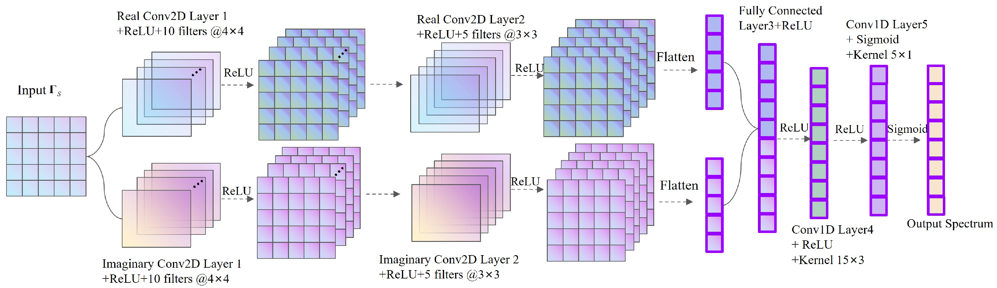
In this section, we propose a SSDC network that formulates the coherent signal DOA estimation as a multi-label classification task. The supervised learning method consists of two stages: the learning stage and the validation stage. The structure diagram of the SSDC network is illustrated in Figure 2. We design a two-input system with $M\ast M$, which includes the real part and the imaginary part of the signal covariance matrix. The two-dimensional convolution is employed to perform feature extraction from the multi-channel input data. Subsequently, Fully connected (FC) layers concatenate the outputs from the real and imaginary parts of the convolutional layers. After one round of a Fully connected layer, a one-dimensional convolution is used for feature fitting. Finally, a pre-selected grid is used to infer the DOA estimation values. As the network runs deeper, to prevent excessive increase in network parameters and the risk of overfitting, we choose a five-layer hidden architecture to achieve a nonlinear representation of the network.

In the training stage of the SSDC network, we assume that the values of the elements in the vector sparse signal $\mathit{\eta }$ are only one at the true source location and zero otherwise. For this, we need to find a relationship from ${\mathbf{\Gamma }}_S$ to sparse signal vector $\mathit{\eta }$, even though it is a black box. According to the well-known universal approximation theorem [31], a feedforward network with a single hidden layer can approximate continuous functions on compact subsets of ${\mathbb{R}}^n$. For multi-layer networks, we define nonlinear function f as a mapping from the input space to the output space, i.e., $f:{\mathbf{\Gamma }}_S\to \mathit{\eta }$, and it is parametrized using a five-layer SSDC model, i.e.,

$${\mathit{\gamma }}_1=f_2\left(f_1\left({\mathbf{X}}^1\right)\right),$$

(8)

$${\mathit{\gamma }}_2=f_2\left(f_1\left({\mathbf{X}}^2\right)\right),$$

(9)

$$\mathit{\eta }=f_5\left(f_4\left(f_3\left(\mathit{\gamma }\right)\right)\right)\in {\mathbb{C}}^{L\times 1},$$

(10)

where ${\mathit{\gamma }}_1$ and ${\mathit{\gamma }}_2$ are the outputs of inputs ${\mathbf{X}}^1=real\left({\mathbf{\Gamma }}_S\right)$ and ${\mathbf{X}}^2=imag\left({\mathbf{\Gamma }}_S\right)$, respectively. $\mathit{\gamma }=\left[\mathrm{Flatten}\left({\mathit{\gamma }}_1\right);\mathrm{Flatten}\left({\mathit{\gamma }}_2\right)\right]$ is the input of the third network layer and the $\mathit{\eta }$ is the final output.

Functions $f_1$ and $f_1$ are based on 2D-convolution architectures and are performed in parallel depending on the real and imaginary parts, which consist of 10 and 5 filters, respectively. Then, they follow a Rectified Linear Unit (ReLU) layer that applies the activation function to the variables from the previous layer. The output of the ith layer is given:

$${\mathbf{o}}^i={\sigma }_i\left({\mathbf{K}}^i\ast {\mathbf{o}}^{i-1}+{\mathbf{b}}_{2\mathrm{D}-\mathrm{C}}^i\right),i=1,2.$$

(11)

Kernel ${\mathbf{K}}^i$ is a 2D matrix of the size of $\kappa \times \kappa$. We employ $\kappa =4$ for $f_1\left(·\right)$ and $\kappa =3$ for the second convolution layers $f_2\left(·\right)$. The stride s is set to $s=1$ with no padding, and ${\mathbf{b}}_{2\mathrm{D}-\mathrm{C}}^i,i=1,2$ represent the bias of the ith layer. Subsequently, we flatten the results obtained from the double parallel convolutions and concatenate them into a single dataset, then enter the third layer, a Fully connected network, represented as

$${\mathbf{o}}^i={\sigma }_i\left({\mathbf{W}}^i\ast {\mathbf{o}}^{i-1}+{\mathbf{b}}_{\mathrm{FC}}^i\right),i=3.$$

(12)

Here, ${\mathbf{W}}^i$ and ${\mathbf{b}}_{\mathrm{FC}}^i$ represent the weight and bias of the ith layer. $f_3\left(·\right)$ is a dense layer with L neurons, followed by a ReLU layer. Thereafter, the proposed $f_4$ and $f_5$ structures are based on the standard 1D convolution architecture, which consists of three and one filters, respectively, i.e.,

$${\mathbf{o}}^i=P\left({\sigma }_i\left({\mathrm{N}}^i\ast {\mathbf{o}}^{i-1}+{\mathbf{b}}_{1\mathrm{D}-\mathrm{C}}^i\right)\right),i=4,5.$$

(13)

Kernel ${\mathrm{N}}^i$ is a vector of size $\kappa \times 1$. We employ $\kappa =15$ for $f_4\left(·\right)$ and $\kappa =5$ for layers $f_5\left(·\right)$. Stride $s=1$ with padding operator $P\left(·\right)$ restores the output of activation function to the original input size by applying zero-padding at the borders. In addition, ${\mathbf{b}}_{1\mathrm{D}-\mathrm{C}}^i,i=4,5$ represent the bias. The all activation function can be expressed as

$${\sigma }_i\left(z\right)=\left\{\begin{array}{c}\mathrm{ReLU}\left(z\right),i=1,2,3,4.\\ \mathrm{Sigmoid}\left(z\right),i=5.\end{array}\right.$$

(14)

The final output layer, $f_5\left(·\right)$, consists of L neurons in a Conv1D layer, followed by the sigmoid activation function. The sigmoid function, defined as $s\left(z\right)=z/\left(e^z+1\right)$, is applied to the values from the preceding layer, returning values within $[0,1]$, representing the probability of each entry in the predicted label. We define the output layer as ${\mathbf{o}}^5=\tilde{\mathit{\eta }}$. Like most supervised learning approaches, the SSDC network trains on the offline dataset ${\mathcal{D}}_{train}=\left\{\left({\mathbf{\Gamma }}_S^1,{\mathit{\eta }}^1\right),\left({\mathbf{\Gamma }}_S^2,{\mathit{\eta }}^2\right),\cdots ,\left({\mathbf{\Gamma }}_S^D,{\mathit{\eta }}^D\right)\right\}$ where D denotes the batch size and parameters $\mathbf{J}={\left\{{\mathcal{W}}^i,{\mathbf{b}}^i\right\}}_{i=1}^5$ with sets of weight ${\left\{{\mathcal{W}}^i\right\}}_{i=1}^5=\left\{{\mathbf{K}}^1,{\mathbf{K}}^2,{\mathbf{W}}^3,{\mathbf{N}}^4,{\mathbf{N}}^5\right\}$ and bias ${\left\{{\mathbf{b}}^i\right\}}_{i=1}^5=\left\{{\mathbf{b}}_{2\mathrm{D}-\mathrm{C}}^1,{\mathbf{b}}_{2\mathrm{D}-\mathrm{C}}^2,{\mathbf{b}}_{\mathrm{FC}}^3,{\mathbf{b}}_{1\mathrm{D}-\mathrm{C}}^4,{\mathbf{b}}_{1\mathrm{D}-\mathrm{C}}^5\right\}$ use backpropagation, minimizing the Mean Square Error (MSE) as the loss function between the reconstructed spectrum $\tilde{\mathit{\eta }}$ and the original $\mathit{\eta }$, as shown in [20], i.e.,

$${\mathbf{J}}^{\ast }=\underset{\mathbf{J}}{argmin}\frac{1}{D}\sum _{j=1}^D{∥{\mathit{\eta }}^j-{\tilde{\mathit{\eta }}}^j∥}^2.$$

(15)

The MSE is an appropriate criterion for minimizing the error between the learning target and the true target. To continuously reduce the loss function $\iota \left(\mathit{\eta }-\tilde{\mathit{\eta }}\right)={∥{\mathit{\eta }}^j-{\tilde{\mathit{\eta }}}^j∥}^2$, backpropagation is used to update the weight and bias vectors. The update process is as follows:

$${\mathcal{W}}^i={\mathcal{W}}^i-\xi \frac{\partial \iota \left(\mathit{\eta }-\tilde{\mathit{\eta }}\right)}{\partial {\mathcal{W}}^i},$$

(16)

and

$${\mathbf{b}}^i={\mathbf{b}}^i-\xi \frac{\partial \iota \left(\mathit{\eta }-\tilde{\mathit{\eta }}\right)}{\partial {\mathbf{b}}^i},$$

(17)

$\frac{\partial \iota \left(\mathit{\eta }-\tilde{\mathit{\eta }}\right)}{\partial {\mathcal{W}}^i}$ and $\frac{\partial \iota \left(\mathit{\eta }-\tilde{\mathit{\eta }}\right)}{\partial {\mathbf{b}}^i}$ are the partial derivatives of the parameters with respect to the ith layer neuron, represented as $\nabla \iota \left(\mathit{\eta }-\tilde{\mathit{\eta }}\right)$, reflecting the sensitivity of the final loss to the ith layer neuron. $\xi$ represents the learning rate.

In addition, this paper adopts an adaptive moment estimation algorithm called Adam [32] to optimize the parameters of the SSDC network. Since the learning rate is a crucial parameter during neural network optimization, setting it too high may cause the loss function not to converge, while setting it too low may result in slow convergence of the loss function. Therefore, we employ a dynamically changing learning rate to adaptively adjust the convergence of the loss function. Assuming $\mathbf{M}$ represents the first moment of the partial derivative and $\mathbf{G}$ represents the second moment of the partial derivative, the Adam algorithm combines the RMSprop algorithm and momentum-based methods. To ensure that each update is related to historical values, it performs exponential moving average on both the gradient and the square of the gradient, as follows:

$${\mathbf{M}}_m={\lambda }_1{\mathbf{M}}_{m-1}+\left(1-{\lambda }_1\right)\nabla \iota \left(\mathit{\eta }-\tilde{\mathit{\eta }}\right)$$

(18)

and

$${\mathbf{G}}_m={\lambda }_2{\mathbf{G}}_{m-1}+\left(1-{\lambda }_2\right){\left[\nabla \iota \left(\mathit{\eta }-\tilde{\mathit{\eta }}\right)\right]}^2$$

(19)

where ${\lambda }_1$ and ${\lambda }_2$ are the decay rates for the two moving averages, with this paper using ${\lambda }_1=0.9$ and ${\lambda }_2=0.999$, and m is the mth of iterations. Then, the initial sliding value is corrected, that is,

$${\tilde{\mathbf{M}}}_m=\frac{{\mathbf{M}}_m}{1-{\lambda }_1^m},$$

(20)

and

$${\tilde{\mathbf{G}}}_m=\frac{{\mathbf{G}}_m}{1-{\lambda }_2^m}.$$

(21)

Finally, the parameters are updated

$$\left\{{\mathcal{W}}^i,{\mathbf{b}}^i\right\}=\left\{{\mathcal{W}}^i,{\mathbf{b}}^i\right\}-\frac{\xi }{\sqrt{{\tilde{\mathbf{G}}}_m+\epsilon }}·{\tilde{\mathbf{M}}}_m$$

(22)

and $\epsilon$ is a very small number (usually $\epsilon =1e-8$) to avoid having a denominator of zero.

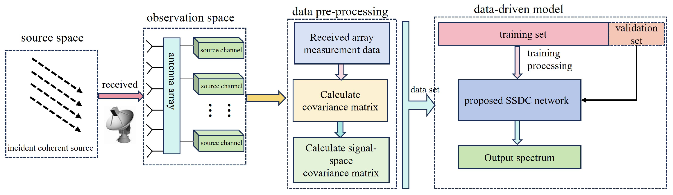
Remark:Figure 3 depicts a fabricated prototype picture of the proposed SSDC network for coherent DOA estimation. When a coherent signal incident on a uniform linear array is considered, the received data need to be preprocessed first. This process requires the covariance matrix to be derived from the received data, and then the signal-space covariance matrix is calculated according to ${\mathbf{\Gamma }}_S={\tau }_1{\mathbf{u}}_1{\mathbf{u}}_1^H\in {\mathbb{C}}^{M\times M}$. The data corresponding to the range of incident DOA are subjected to this preprocessing process; a random $80\%$ of the signal spatial covariance and the corresponding spatially sparse signal data are used to enter the proposed SSDC network for training and $20\%$ of the preprocessed data is randomly selected for validation.

4. Simulation Results

In this section, we carry out several simulations to discuss the performance of the proposed SSDC network, the SS-MUSIC method [26], and DL-based DOA estimation methods, i.e., ASL (we use ASL2) [29], DCN [20], and DNN [19]. The root mean square error (RMSE) and MSE are used to evaluate the performance of these algorithms, which is

$$\mathrm{RMSE}=\sqrt{\frac{1}{Q·\mathrm{MC}}\sum _{q=1}^Q\sum _{n=1}^{\mathrm{MC}}{\left({\widehat{\theta }}_{qn}-{\theta }_q\right)}^2}$$

(23)

$$\mathrm{MSE}=\frac{1}{Q·\mathrm{MC}}\sum _{q=1}^Q\sum _{n=1}^{\mathrm{MC}}{\left({\widehat{\theta }}_{qn}-{\theta }_q\right)}^2$$

(24)

where ${\theta }_q$ and ${\widehat{\theta }}_{qn}$ denote the real and estimated DOAs in the nth Monte Carlo (MC) simulation experiment, respectively.

The Cramér–Rao Bound (CRB) provides a lower bound on the covariance matrix of for any unbiased estimator [33]. In this paper, the CRB is used in the case of large snapshots of the estimated variance approximation using the stochastic maximum likelihood algorithm [33], represented as

$$\mathbf{CRB}\left(\theta \right)=\frac{{\sigma }_n^2}{2T}{\left\{Re\left[\mathbf{H}\odot {\mathbf{G}}^T\right]\right\}}^{-1},$$

(25)

with

$$\mathbf{H}={\mathbf{h}}^H\left({\mathbf{I}}_M-\mathbf{A}{\left({\mathbf{A}}^H\mathbf{A}\right)}^{-1}{\mathbf{A}}^H\right)\mathbf{h},$$

(26)

and

$$\mathbf{G}={\mathbf{R}}_s^H{\mathbf{A}}^H{\mathbf{R}}^{-1}\mathbf{A}{\mathbf{R}}_s,$$

(27)

where $\mathbf{h}=\left[\frac{\partial \mathbf{a}\left({\theta }_1\right)}{\partial {\theta }_1},\cdots ,\frac{\partial \mathbf{a}\left({\theta }_Q\right)}{\partial {\theta }_Q}\right]\in {\mathbb{C}}^{M\times Q}$ is the first-order derivative of the direction vector, $\mathbf{R}$ is the covariance matrix calculated by Equation (3), ${\mathbf{R}}_s$ is a singular matrix with a rank of one.

4.1. Experiment Setup

To train the proposed SSDC network, we consider the grid with resolution of $\Delta \phi =\left\{1^{\circ },2^{\circ },\cdots ,{39}^{\circ },{40}^{\circ }\right\}$ and define a narrow grid scope $\mathit{\phi }\in \left\{-{30}^{\circ },-{29}^{\circ },\cdots ,{29}^{\circ }\right\}$ with $L_{max}={60}^{\circ }$. For the simulations, we employ a ULA with $M=8$ sensors, $T=256$, array spacing $d=0.5$ m, and signal carrier wavelength $\lambda =1$ m.

For the training dataset, we select $Q=2$ coherent sources with $\mathbf{\alpha }={\left[1,1\right]}^T$. The first and second sources are uniformly generated within the ranges $\left[-{30}^{\circ },{29}^{\circ }-\Delta \phi \right]$ and $\left[-{30}^{\circ }+\Delta \phi ,{29}^{\circ }\right]$ with a step of $1^{\circ }$, and 10 groups of fixed snapshots are collected with SNR randomly distributed between −20 dB and 0 dB. Based on Python 3.10 and the Adam optimizer, we utilize Keras 2.12.0 and its embedded tools for gradient computation to implement the training of SSDC network. The data are generated by the operating environment “12th Gen Intel(R) Core(TM) i7-12700H 2.30 GHz processor with a 64-bit operating system MATLAB 2022a”, and the sample datasets consist of a total of 15,800 measurement vectors. In addition, we adopt mini-batch training with a batch size of 64 and conduct 500 training epochs.

4.2. MSE during Training and Validation

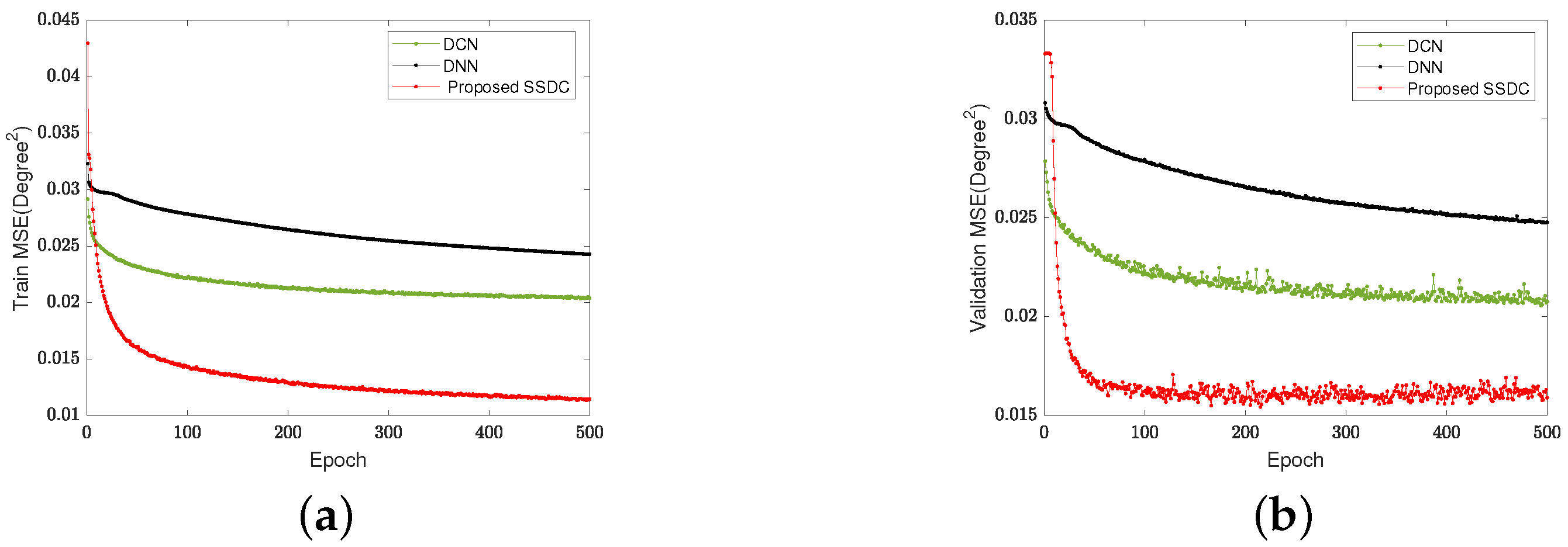
Figure 4 illustrates the changes in MSE during the training and validation of the DCN [20], the DNN [19], and the proposed SSDC methods.

The DNN-based framework consists of a multi-task autoencoder and a series of parallel multilayer classifiers [19]. The spacing of the array elements of the ULA in the DNN model is half a wavelength, and the potential space is divided into six subregions of equal spatial extent. The number of hidden layers in each subregion is two, and the sizes of the hidden and output layers of each classifier are 30, 20, and 20, respectively. All the weights and biases of the DNN are randomly initialized with a uniform distribution between −0.1 and 0.1.

The DCN-based framework [20] can learn inverse transformations from large training datasets, considering the spatial sparsity of the incident signal. The DOA estimation problem is transformed into a sparse linear inverse problem by introducing a spatial overcomplete formulation. Compared with the traditional iteration-based sparse recovery algorithms, the DCN-based method requires only feed-forward computation to realize real-time direction measurement. The DCN network has four hidden layers and one output layer with convolutional kernels of 25 × 12, 15 × 6, 5 × 3, 3 × 1, and an output dimension of 60 × 1, respectively.

As can be seen from Figure 4, the proposed SSDC network exhibits lower MSE on both the training and validation sets compared to the other two methods. The generated data are randomly partitioned into two sets: $80\%$ is allocated for the training set, while the remaining $20\%$ is assigned to the validation set. Figure 4a provides a clear visualization of the training process, where the initial higher loss values are attributed to the random initialization of model parameters and limited understanding of data patterns. As training progresses, the model gradually learns the data features, resulting in a steady reduction in the loss function.

To prevent overfitting during the training process, a validation dataset is used to evaluate the model’s performance on unused data. Figure 4b displays the model’s loss function performance on the validation data as the training advances. While the training loss might fluctuate, the overall trend shows a decreasing pattern. Furthermore, the proposed SSDC network exhibits lower MSE values on both the training and validation sets compared to the other two methods.

To evaluate the computational complexity of the proposed SSDC algorithm, in

Table 1. Average running time.

		Method	ASL [29]	DNN [19]	DCN [20]	SSDC	SS-MUSIC [26]
	Time
Item
Total params			585,276	32,466	1801	6774	∖
Train time			1236.9480 s	1390.2328 s	1023.6829 s	713.2126 s	∖
Test time			0.0688 s	0.2340 s	0.0960 s	0.0722 s	0.3288 s

, we record the running time required by all the related algorithms (average of 50 tests). It can be seen that the running time of the proposed SSDC algorithm is only a fraction of the SS-MUSIC algorithm [26]. Moreover, the ASL algorithm [29] has the longest train time due to its very large number of parameters. Next, multiple DNNs (six DNNs in [19]) need to be trained, so SSDC is also more efficient than [19]. Furthermore, compared to the DCN algorithm [20], although the proposed SSDC has more parameters, SSDC reduces the computational dimensions by processing the real and imaginary parts separately, and thus SSDC is more efficient than DCN.

4.3. Experiment with the Same Number of Coherent Sources in the Test Set As in the Training Set

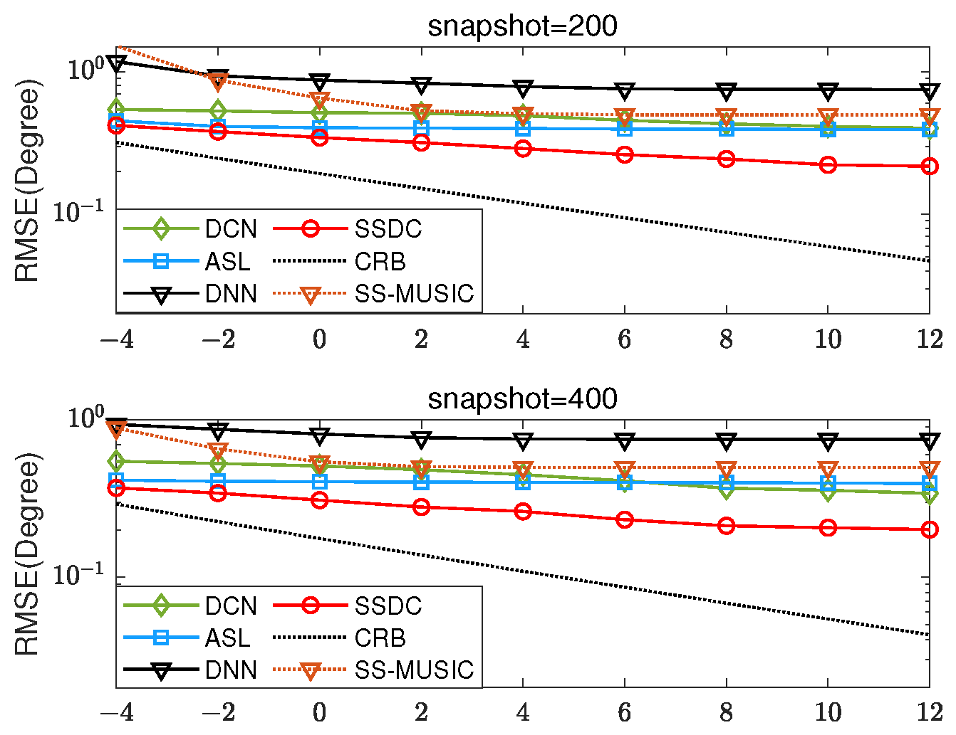
Firstly, two coherent sources with DOAs $-{5.5}^{\circ }$ and ${8.5}^{\circ }$ and SNR within $\left[-4,12\right]$ dB are considered. As shown in Figure 5, we conduct 500 independent MC simulation experiments with snapshot numbers set at 200 and 400. The proposed SSDC method has better estimation performance compared to the SS-MUSIC method and other three data-driven methods. Figure 5 shows the RMSE’s variation of the proposed SSDC network at different SNR levels. As the SNR increases, the RMSE shows a decreasing trend, i.e., the RMSE is smaller at higher SNRs. This indicates that the SSDC network estimator performs better and can estimate the DOAs more accurately when the signal is relatively strong and the noise is weak. Therefore, there is a negative correlation between the SNR and the RMSE, and a high SNR usually corresponds to a low RMSE.

Table 2. RMSE for various SNRs for two coherent sources with DOAs $-{5.5}^{\circ }$ and ${8.5}^{\circ }$.

		Snapshot	Snapshot = 200					Snapshot = 400
	RMSE
Method
SNR			DCN	ASL	DNN	SS-MUSIC	SSDC	DCN	ASL	DNN	SS-MUSIC	SSDC
−4			0.5448	0.4530	1.1791	1.5217	0.4204	0.5462	0.4145	0.9382	0.8892	0.3695
−2			0.5317	0.4142	0.9368	0.8740	0.3809	0.5288	0.4074	0.8720	0.6553	0.3428
0			0.5165	0.4052	0.8745	0.6542	0.3457	0.5099	0.4052	0.8142	0.5423	0.3092
2			0.5125	0.4026	0.8328	0.5332	0.3188	0.4828	0.4020	0.7721	0.5049	0.2795
4			0.4924	0.4004	0.7884	0.5280	0.2894	0.4486	0.4019	0.7571	0.5020	0.2621
6			0.4568	0.3968	0.7605	0.5190	0.2624	0.4104	0.4002	0.7538	0.5000	0.2323
8			0.4319	0.3967	0.7523	0.5125	0.2446	0.3683	0.3995	0.7522	0.5000	0.2124
10			0.4136	0.3940	0.7522	0.5000	0.2225	0.3571	0.3969	0.7521	0.5000	0.2065
12			0.4024	0.3938	0.7519	0.5000	0.2174	0.3414	0.3948	0.7518	0.5000	0.2009

provides the visualized RMSE values of Figure 5. It can be more clearly observed that the proposed SSDC network has the lowest RMSE in the range of −4 to 12 dB.

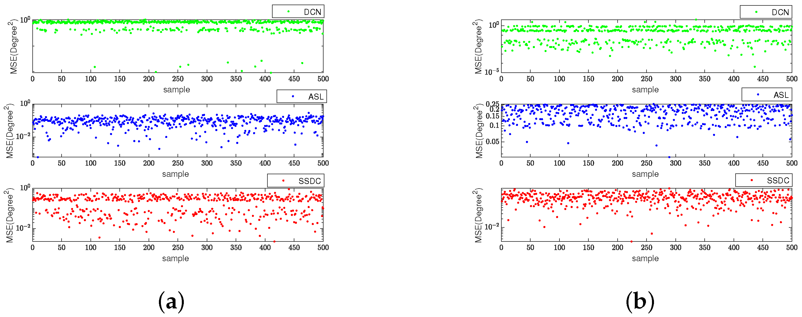
For enhanced result visualization, Figure 6 displays the corresponding estimated MSE for the two sources. The first source is characterized by direction ${\theta }_1=-{5.5}^{\circ }+\mathit{randn}$, while the second source is ${\theta }_1+\Delta \phi$ with $\Delta \phi =6^{\circ }$ in Figure 6a and $\Delta \phi ={21}^{\circ }$ in Figure 6b. The snapshot is 256, SNR = 0 dB. We observe that the estimated MSE of the DOA estimation obtained by our method optimizes the estimation at both large and small angular intervals.

4.4. Experiment with a Different Number of Coherent Sources in the Test and Training Sets

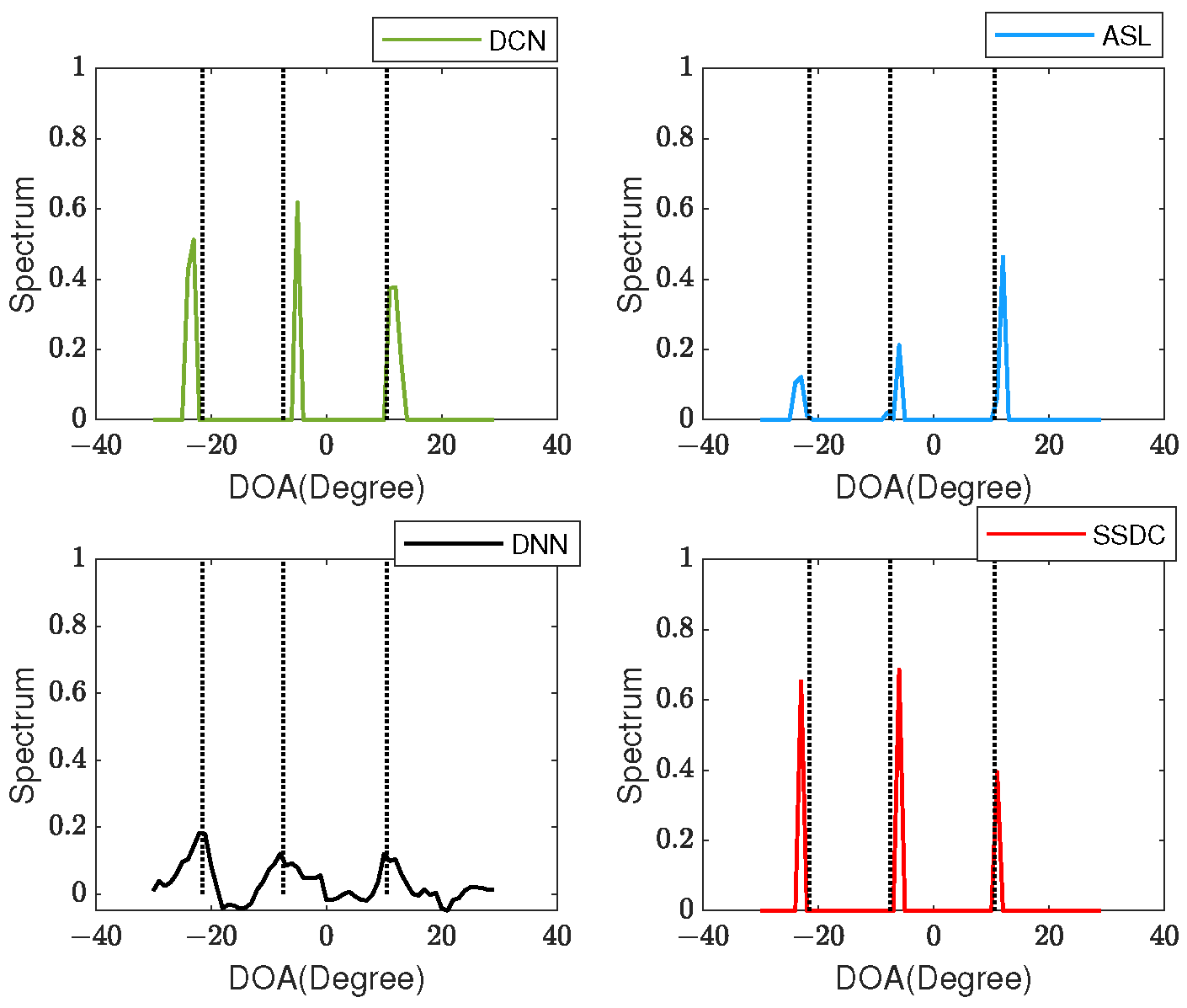
Next, spectral peaks are tested in three coherent signals with DOAs of $[-{21.5}^{\circ },-{7.5}^{\circ },$${10.5}^{\circ }]$, as shown in Figure 7, where SNR = 10 dB, the number of snapshots is 256. When the number of signals $K⩾3$, the SS-MUSIC algorithm does not work well in this case due to the total number of array elements $M=8$, so it is not used for comparison. Even in the case of a mismatch between the number of test sources and the number of training sources, the proposed method could search for sharper peaks.

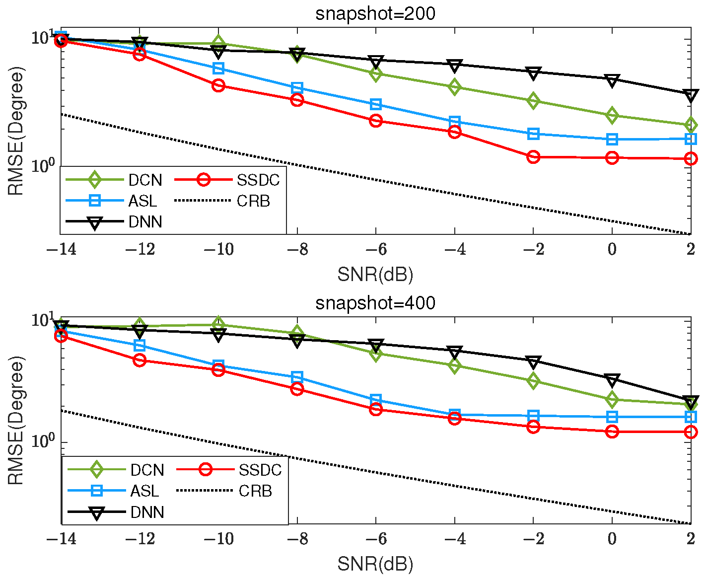
Three coherent signals located at $-{21.5}^{\circ }$, $-{7.5}^{\circ }$, and ${10.5}^{\circ }$ with SNRs within $\left[-14,2\right]$ dB are considered, and for the RMSE of each SNR, we perform 500 independent MC simulation experiments, as shown in Figure 8. Similarly, the snapshot numbers are set to 200 and 400, respectively. As the SNR and snapshot increase, the proposed SSDC method exhibits higher estimation accuracy compared to the ASL algorithm, which is also designed for coherent signal estimation. Moreover, it can be seen from Figure 8 that the performance of the proposed SSDC network estimator decreases the RMSE as the SNR increases.

Table 3. RMSE for various SNRs for three coherent sources with DOAs $\left[-{21.5}^{\circ },-{7.5}^{\circ },{10.5}^{\circ }\right]$.

		Snapshot	Snapshot = 200				Snapshot = 400
	RMSE
Method
SNR			DCN	ASL	DNN	SSDC	DCN	ASL	DNN	SSDC
−14			9.8974	10.3946	10.0370	9.6787	9.0068	8.3523	9.3075	7.6015
−12			9.1955	8.2625	9.4923	7.6144	9.1493	6.3520	8.5037	4.7888
−10			9.2857	5.9264	8.1795	4.3582	9.4124	4.3264	7.9674	3.9796
−8			7.6149	4.18250	7.8453	3.3594	7.9726	3.4661	7.1206	2.7717
−6			5.4049	3.1088	6.8769	2.3168	5.4628	2.2495	6.5506	1.8838
−4			4.2463	2.2809	6.3749	1.8961	4.3471	1.7000	5.7563	1.5841
−2			3.3147	1.8345	5.5767	1.1746	3.2389	1.6672	4.7569	1.3516
0			2.5506	1.6609	4.9036	1.1926	2.2688	1.6304	3.3722	1.2355
2			2.1431	1.6710	3.7398	1.2104	2.0703	1.6321	2.2262	1.2239

provides the visualized RMSE values of Figure 8. It can be more clearly observed that the proposed SSDC network has the lowest RMSE in the range of −14 to 2 dB. Despite the lower SNR, the proposed SSDC network still has the optimal performance compared to the other three methods.

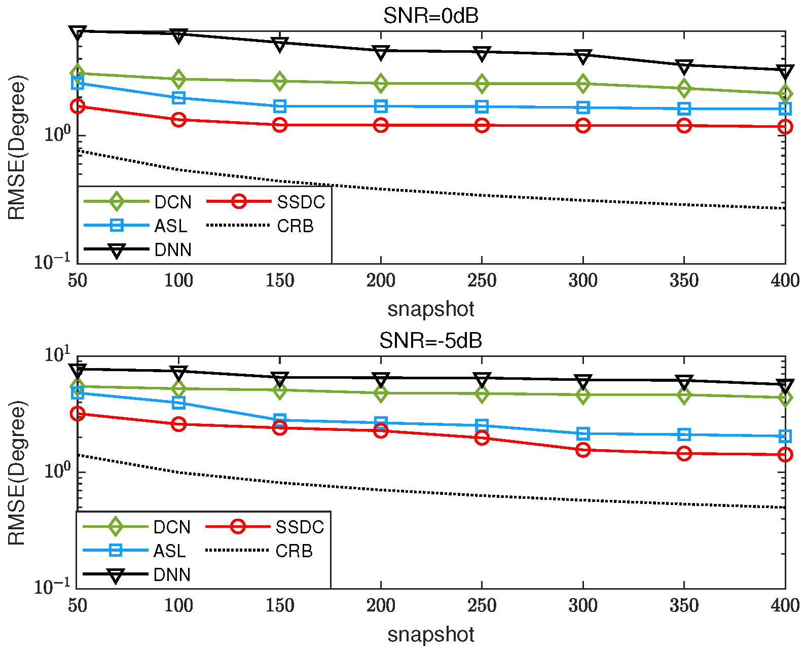
Finally, we test snapshots with an interval of 50 in the range of $\left[50,400\right]$ and perform 500 independent Monte Carlo (MC) simulations at SNRs of −5 dB and 0 dB, respectively. The RMSE results are shown in Figure 9. As the number of snapshots increases, the proposed SSDC algorithm is significantly robust and performs optimally, even in scenarios where the number of test targets and training targets mismatch.

5. Conclusions

In this paper, we proposed a data-driven approach for coherent direction of arrival (DOA) estimation, improving the coherent signal DOA estimation accuracy compared to the SS-MUSIC and recently reported data-driven algorithms. Our novel neural network, the signal-space deep convolutional (SSDC) network, effectively handles coherent signals by using the signal-space covariance matrix as input. This reduces noise interference and enables efficient learning of angular features, leading to improved DOA estimation accuracy. Unlike conventional neural networks, we partitioned the input signal-space covariance matrix into real and imaginary part matrices, allowing for independent two-dimensional convolution operations that maximize the utilization of input data features. Furthermore, we considered the spatial sparsity of the array output and performed spectral peak searches to accurately determine relevant DOAs. Simulation results demonstrate the superiority of our SSDC network over existing deep learning coherence DOA approaches. This research advances DOA estimation techniques and opens avenues for improved performance in various applications, such as wireless communications, radar systems, and acoustic signal processing.

References

- Krim, H.; Viberg, M. Two decades of array signal processing research: The parametric approach. IEEE Signal Process. Mag. 1996, 13, 67–94. [Google Scholar] [CrossRef]
- Dong, X.; Zhao, J.; Sun, M.; Zhang, X.; Wang, Y. A modified δ-generalized labeled multi-Bernoulli filtering for multi-source DOA tracking with coprime array. IEEE Trans. Wirel. Commun. 2023, 22, 9424–9437. [Google Scholar] [CrossRef]
- Yang, B.; Zhu, S.; He, X.; Lan, L.; Li, X. Cognitive FDA-MIMO radar network for target discrimination and tracking with main-lobe deceptive trajectory interference. IEEE Trans. Aerosp. Electron. Syst. 2023, 59, 4207–4222. [Google Scholar] [CrossRef]
- Famoriji, O.J.; Shongwe, T. Deep learning approach to source localization of electromagnetic waves in the presence of various sources and noise. Symmetry 2023, 15, 1534. [Google Scholar] [CrossRef]
- Ibrahim, M.; Ramireddy, V.; Lavrenko, A.; König, J.; Römer, F.; Landmann, M.; Grossmann, M.; Del Galdo, G.; Thomä, R.S. Design and analysis of compressive antenna arrays for direction of arrival estimation. Signal Process. 2017, 138, 35–47. [Google Scholar] [CrossRef]
- Schmidt, R.O. Multiple emitter location and signal parameter estimation. IEEE Trans. Antennas Propag. 1986, 34, 276–280. [Google Scholar] [CrossRef]
- Roy, R.; Kailath, T. ESPRIT-estimation of signal parameters via rotational invariance techniques. IEEE Trans. Acoust. Speech Signal Process. 1989, 37, 984–995. [Google Scholar] [CrossRef]
- Zeng, W.J.; So, H.C.; Huang, L. lp-MUSIC: Robust direction-of-arrival estimator for impulsive noise environments. IEEE Trans. Signal Process. 2013, 61, 4296–4308. [Google Scholar] [CrossRef]
- Yang, Z.; Xie, L. Enhancing sparsity and resolution via reweighted atomic norm minimization. IEEE Trans. Signal Process. 2015, 64, 995–1006. [Google Scholar] [CrossRef]
- Liu, Z.M.; Huang, Z.T.; Zhou, Y.Y. Sparsity-inducing direction finding for narrowband and wideband signals based on array covariance vectors. IEEE Trans. Wirel. Commun. 2013, 12, 1–12. [Google Scholar] [CrossRef]
- Yang, Z.; Xie, L.; Zhang, C. Off-grid direction of arrival estimation using sparse Bayesian inference. IEEE Trans. Signal Process. 2012, 61, 38–43. [Google Scholar] [CrossRef]
- Aghababaiyan, K.; Shah-Mansouri, V.; Maham, B. High-precision OMP-based direction of arrival estimation scheme for hybrid non-uniform array. IEEE Commun. Lett. 2019, 24, 354–357. [Google Scholar] [CrossRef]
- Tropp, J.A.; Gilbert, A.C. Signal recovery from random measurements via orthogonal matching pursuit. IEEE Trans. Inf. Theory 2007, 53, 4655–4666. [Google Scholar] [CrossRef]
- Shi, Y.; Mao, X.P.; Qian, C.; Liu, Y.T. Robust relaxation for coherent DOA estimation in impulsive noise. IEEE Signal Process. Lett. 2019, 26, 410–414. [Google Scholar] [CrossRef]
- LeCun, Y.; Bengio, Y.; Hinton, G. Deep learning. Nature 2015, 521, 436–444. [Google Scholar] [CrossRef] [PubMed]
- Shmuel, D.H.; Merkofer, J.P.; Revach, G.; van Sloun, R.J.; Shlezinger, N. Deep root MUSIC algorithm for data-driven DoA estimation. In Proceedings of the ICASSP 2023—2023 IEEE International Conference on Acoustics, Speech and Signal Processing (ICASSP), Rhodes Island, Greece, 4–10 June 2023; pp. 1–5. [Google Scholar]
- Randazzo, A.; Abou-Khousa, M.A.; Pastorino, M.; Zoughi, R. Direction of arrival estimation based on support vector regression: Experimental validation and comparison with MUSIC. IEEE Antennas Wirel. Propag. Lett. 2007, 6, 379–382. [Google Scholar] [CrossRef]
- Kase, Y.; Nishimura, T.; Ohgane, T.; Ogawa, Y.; Kitayama, D.; Kishiyama, Y. DOA estimation of two targets with deep learning. In Proceedings of the 2018 15th Workshop on Positioning, Navigation and Communications (WPNC), Bremen, Germany, 23–24 October 2018; pp. 1–5. [Google Scholar]
- Liu, Z.M.; Zhang, C.; Philip, S.Y. Direction-of-arrival estimation based on deep neural networks with robustness to array imperfections. IEEE Trans. Antennas Propag. 2018, 66, 7315–7327. [Google Scholar] [CrossRef]
- Wu, L.; Liu, Z.M.; Huang, Z.T. Deep convolution network for direction of arrival estimation with sparse prior. IEEE Signal Process. Lett. 2019, 26, 1688–1692. [Google Scholar] [CrossRef]
- Papageorgiou, G.K.; Sellathurai, M.; El-r, Y.C. Deep networks for direction-of-arrival estimation in low SNR. IEEE Trans. Signal Process. 2021, 69, 3714–3729. [Google Scholar] [CrossRef]
- Feintuch, S.; Tabrikian, J.; Bilik, I.; Permuter, H. Neural network-based DOA estimation in the presence of non-Gaussian interference. IEEE Trans. Aerosp. Electron. Syst. 2023, 60, 119–132. [Google Scholar] [CrossRef]
- Merkofer, J.P.; Revach, G.; Shlezinger, N.; Routtenberg, T.; van Sloun, R.J. DA-MUSIC: Data-driven DoA estimation via deep augmented MUSIC algorithm. IEEE Trans. Veh. Technol. 2023, 73, 2771–2785. [Google Scholar] [CrossRef]
- Labbaf, N.; Oskouei, H.D.; Abedi, M.R. Robust DOA estimation in a uniform circular array antenna with errors and unknown parameters using deep learning. IEEE Trans. Green Commun. Netw. 2023, 7, 2143–2152. [Google Scholar] [CrossRef]
- SongGong, K.; Wang, W.; Chen, H. Acoustic source localization in the circular harmonic domain using deep learning architecture. IEEE/ACM Trans. Audio Speech Lang. Process. 2022, 30, 2475–2491. [Google Scholar] [CrossRef]
- Pillai, S.U.; Kwon, B.H. Forward/Backward spatial smoothing techniques for coherent signal Identification. IEEE Trans. Acoust. Speech Signal Process. 1989, 37, 8–15. [Google Scholar] [CrossRef]
- Pan, J.; Sun, M.; Wang, Y.; Zhang, X. An Enhanced Spatial Smoothing Technique With ESPRIT Algorithm for Direction of Arrival Estimation in Coherent Scenarios. IEEE Trans. Signal Process. 2020, 68, 3635–3643. [Google Scholar] [CrossRef]
- Pan, J.; Sun, M.; Wang, Y.; Zhang, X.; Li, J.; Jin, B. Simplified spatial smoothing for DOA estimation of coherent signals. IEEE Trans. Circuits Syst. II Express Briefs 2022, 70, 841–845. [Google Scholar] [CrossRef]
- Xiang, H.; Chen, B.; Yang, M.; Xu, S. Angle separation learning for coherent DOA estimation with deep sparse prior. IEEE Commun. Lett. 2020, 25, 465–469. [Google Scholar] [CrossRef]
- Lee, K. Deep learning-aided coherent direction-of-arrival estimation with the FTMR algorithm. IEEE Trans. Signal Process. 2022, 70, 1118–1130. [Google Scholar]
- Hornik, K.; Stinchcombe, M.; White, H. Multilayer feedforward networks are universal approximators. Neural Netw. 1989, 2, 359–366. [Google Scholar] [CrossRef]
- Kingma, D.P.; Ba, J. Adam: A method for stochastic optimization. arXiv 2014, arXiv:1412.6980. [Google Scholar]
- Weiss, A.; Friedlander, B. On the Cramer-Rao Bound for direction finding of correlated signals. IEEE Trans. Signal Process. 1993, 41, 495. [Google Scholar] [CrossRef]
Figure 1.
Scene of a uniform linear array receiving signals.
Figure 2.
Proposed signal-space deep convolution (SSDC) network.
Figure 3.
Overall SSDC framework for coherent DOA estimation.
Figure 4.
MSE of training and validation. (a) The training MSE. (b) The validation MSE.
Figure 5.
RMSE for various SNRs for two coherent sources with DOAs and .
Figure 6.
MSE versus different MC trials for and , , SNR = 0 dB. (a) . (b) .
Figure 7.
Spectrum for three coherent sources with DOAs .
Figure 8.
RMSE for various SNRs.
Figure 9.
RMSE versus the number of snapshots for three coherent sources with DOAs .