Abstract
Human-like automatic deductive reasoning has always been one of the most challenging open problems in the interdisciplinary field of mathematics and artificial intelligence. This paper is the third in a series of our works. We built a neural-symbolic system, named FGeo-DRL, to automatically perform human-like geometric deductive reasoning. The neural part is an AI agent based on deep reinforcement learning, capable of autonomously learning problem-solving methods from the feedback of a formalized environment, without the need for human supervision. It leverages a pre-trained natural language model to establish a policy network for theorem selection and employ Monte Carlo Tree Search for heuristic exploration. The symbolic part is a reinforcement learning environment based on geometry formalization theory and FormalGeo, which models geometric problem solving (GPS) as a Markov Decision Process (MDP). In the formal symbolic system, the symmetry of plane geometric transformations ensures the uniqueness of geometric problems when converted into states. Finally, the known conditions and objectives of the problem form the state space, while the set of theorems forms the action space. Leveraging FGeo-DRL, we have achieved readable and verifiable automated solutions to geometric problems. Experiments conducted on the formalgeo7k dataset have achieved a problem-solving success rate of 86.40%.
1. Introduction
The rapid development of large language models signifies a new potential for machine intelligence in addressing geometric problems. The emergence of ChatGPT has significantly enhanced the ability to effectively solve geometric problems by enabling machines to delve deeper into the understanding of human language [1]. This innovation has paved the way for the application of artificial intelligence in the field of mathematics. Through the language model’s comprehension and analysis of geometric problems [2], users can obtain more intuitive and insightful explanations, along with targeted suggestions, such as selecting appropriate geometric principles or proof methods.
However, it is important to note that, despite the positive role played by large language models in the initial resolution of geometric problems, they are not mathematical experts. The advice they provide should be regarded as inspirational guidance rather than absolute and precise theorem proofs [3]. When dealing with more complex and formal geometric proofs, reliance on professional mathematical knowledge and tools, such as mathematical software and theorem provers, is still necessary.
Nevertheless, exclusive reliance on language models for geometric reasoning casts doubts on the interpretability of theorem application and the feasibility of its execution [4]. The opacity of neural networks obscures our understanding of how they process input problems. Furthermore, the absence of precise metrics for evaluating executable sequences hinders the verification of complete problem resolution through the output theorem sequences. Since logical natural language processing requires step-by-step derivation based on human understanding, directly deducing the solvability of geometric problems via natural language model reasoning remains an elusive goal [5,6].
To address the aforementioned issues, we propose a geometric formal language system called FormalGeo. By transforming natural language and graphical information into a universally machine-processable formal language, we ensure that the formal language remains consistent before and after geometric transformations such as mirroring and rotation, due to the inherent symmetry of geometric shapes. Our formalization system effectively addresses this concern. Subsequently, we have successfully integrated multiple existing geometric datasets, including Geometry3k [2], GeoQA [7], GeoQA+ [8], and online resources. For these dataset resources, Geometry3k, while comprehensive, is relatively small and may not provide enough variety for large model training. GeoQA and GeoQA+ offer a multimodal approach, but they may fall short in interpretability and verifiability when compared to formal systems. To enhance data quality, we conducted processes such as manual annotation, deduplication, and correction, comprehensively optimizing the dataset. Ultimately, we successfully annotated approximately 6981 problems, creating a novel geometric dataset named FormalGeo7k [9]; the dataset can be obtained here: https://github.com/BitSecret/FGPS, (accessed on 2 April 2024).
Due to the extensive need for annotated datasets in training natural language models, the limited dataset annotated through our formal language system is insufficient for complete theorem prediction using natural language models. Our study introduces a novel solution named FGeo-DRL. This system integrates a neural-symbolic framework, which autonomously learns problem-solving strategies for geometric problems without the need for human intervention, thereby significantly surpassing traditional methods. By combining the adaptive learning capability of the AI agent with the structured precision of geometric formal systems, FGeo-DRL not only manages the complexity of geometric reasoning but also adopts an innovative approach by integrating deep reinforcement learning and Monte Carlo Tree Search techniques into geometric reasoning. Simultaneously, reinforcement learning often requires defining a suitable reward function for guidance. In the case of immediate rewards, manually defining them is subjective and faces challenges in dealing with almost infinite state spaces. On the other hand, learning rewards through inverse reinforcement learning requires extensive annotated data and presents interpretability issues [10,11]. We adopt delayed rewards to handle the reward feedback generated during the search. The use of Monte Carlo Tree Search allows us to obtain a search trajectory chain, and the reward value is fed back based on whether the problem is ultimately solved. The search process is guided by the magnitude of rewards generated through multiple simulations [12]. A preprint of this work has also been published and is available for consultation at https://arxiv.org/abs/2402.09051 (accessed on 2 April 2024) [13].
Symmetry plays a crucial role in geometric reasoning, influencing both the understanding and solving of geometric problems. The concept of symmetry, especially in plane geometry, encompasses various transformations such as reflections, rotations, and translations, which preserve certain properties of geometric figures. The integration of symmetry within the FGeo-DRL framework can enhance the system’s ability to recognize and apply symmetric properties and transformations effectively. This can lead to a more robust and intuitive understanding of geometric problems, often reducing the complexity of problem solving by identifying congruent or similar shapes and leveraging symmetrical properties.
In summary, our contributions can be categorized into the following three points:
- We integrated existing well-known datasets and added additional problems beyond those in the field, constructing a larger dataset for geometric problem solving. This dataset comprises a total of 6981 manually annotated and solved geometric problems.
- We established a geometric formal language system (FormalGeo) that guides the transformation of natural language into formal language. Concurrently, we built a geometric problem solver (FGPS) to validate annotated theorem sequences. By annotating the original image and text information of problems into a form understandable by the geometric formal language system, we can input the theorem sequences for validation. This not only ensures the correctness of proofs but also achieves interpretable step-by-step deduction.
- We introduced reinforcement learning, specifically employing a Monte Carlo Tree Search, into geometric automated reasoning. This is executed by conducting heuristic searches in a geometric reasoning environment built upon the FormalGeo system to address the limited annotated data issue.
2. Related Work
2.1. Datasets for Geometry Problems Solving
In the early research on geometric theorem proving [14,15,16], efforts such as those based on symbolic systems like GeoS [17] or Inter-GPS aimed to construct formal language systems. These systems, by building solvers, enabled formal language to prove geometric propositions through logical deduction. However, with the rise of large language models, more recent work, including GeoQA and UniGeo, began treating problems and diagrams as multimodal inputs, generating solution sequences through large models. Although these methods exhibit high generality, they fall short in terms of interpretability and verifiability compared to symbol-based reasoning in formal systems. Past formal systems, designed manually for logical languages, faced limitations in broader application scenarios, resulting in relatively small datasets, such as GeoS with 186 questions and Geometry3k dataset which used by Inter-GPS containing approximately 3002 problems. These datasets appear relatively small when considered in the context of large models relying on extensive corpora. To address this issue, we integrated multiple publicly available geometric problem datasets. Due to the inconsistency in their formats, we manually reannotated them, including Geometry3k, GeoQA, and GeoQA+. Ultimately, we introduced a large-scale public dataset named FormalGeo7k, comprising around 6981 planar geometry problems. Our work is dedicated to addressing the heterogeneity in data sources to create a more unified and comprehensive dataset. This integration process aims to enhance data consistency and comparability, providing a more robust and comprehensive foundation for our research. This approach allows us to more effectively explore and analyze key features and patterns in geometric data.
2.2. Reinforcement Learning for Geometry Problems Solving
In recent years, numerous studies have demonstrated the application of reinforcement learning in the reasoning process. In [18], Monte Carlo simulation was employed for mathematical theorem proving, while deep reinforcement learning was utilized for interactive theorem proving [19] and solving math word problems [20,21]. However, there has been limited exploration of applying reinforcement learning to geometric theorem proving. The most recent work involves using deep reinforcement learning to address geometric problems [22]. In our study, considering the challenges in defining a reward function, we adopt the Monte Carlo method for interactive search. We replace the immediate rewards obtained through the reward function with delayed rewards acquired through the completion of a full round of interactions. The reward is determined by the success of theorem solving in the Monte Carlo Tree Search process [23], akin to the approach used in AlphaGo [12]. This modification allows us to use reward feedback to shorten the length of theorem sequences, ultimately achieving an optimal sequence.
3. Geometry Formal System
In the process of solving geometric problems, mathematical formal systems play a crucial role, facilitating the transformation from information accessible to humans to the formal language comprehensible by machines. Particularly, when solving problems using artificial intelligence, formal systems become pivotal. Simultaneously, the combination of manual annotation and formal systems ensures consistency between the description of geometric problems and the dataset format, eliminating confounding factors for assessing the performance of artificial intelligence models. However, the answers generated by artificial intelligence models need reliable validation. Considering that traditional manual verification methods are both inefficient and error-prone, we have established a geometric problem solver on the basis of FormalGeo to verify answers [9].
3.1. Geometry Formal Language
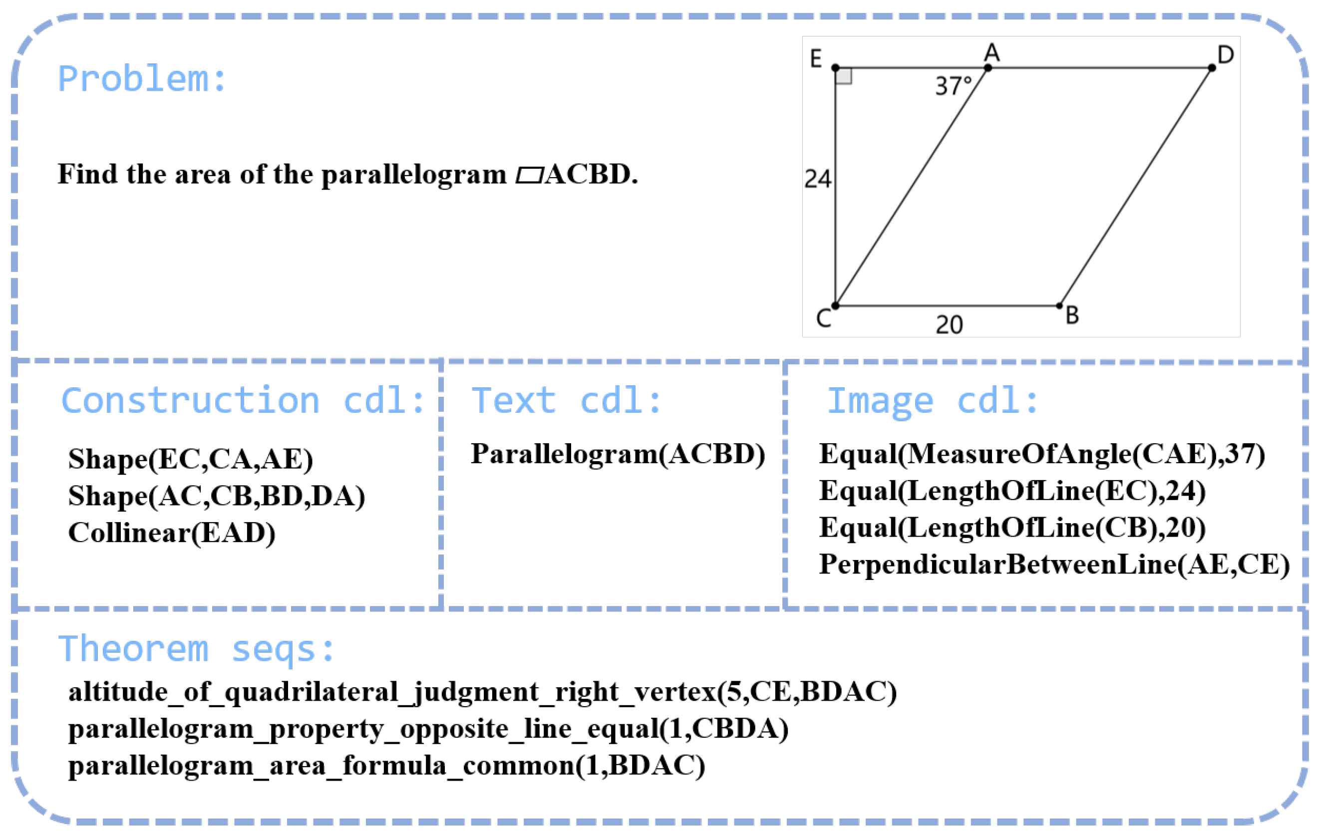
The incorporation of a geometric formal system empowers computers with the capability to comprehend geometric problems, with formal language serving as the bridge between humans and machines. Within the geometric formal system, the formal language consists of Geometric Definition Language (GDL) and Conditional Declaration Language (CDL). As illustrated in Figure 1, CDL is utilized for describing textual and graphical information. GDL, on the other hand, is composed of Predicate Definition Language and Theorem Definition Language. Thus, formal language functions as a bridge between humans and machines.
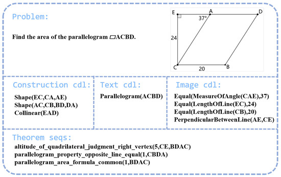
Figure 1.
Formal language for geometry problems. (The letters A to E in parentheses represent points in the geometric figure).
Predicate Definition Language: Predicate Definition Language is employed to describe the direct geometric relationships and attributes among entities. It encompasses predicates that describe the structural aspects of geometric figures. Through structural predicates, one can articulate general relationships, such as coplanarity, shape, and collinearity. These structural predicates can further extend to basic entities like lines, angles, arcs, polygons, circles, and more. In addition to structural predicates, custom predicates can be utilized to automatically expand into other customized relationships. Examples include geometric relationships of custom shapes like right-angled triangles, trapezoids, as well as algebraic relationships.
Theorem Definition Language: It is comprised of premises and conclusions, with geometric relationships and attributes serving as premises, and conclusions being extended under the judgment rules of the theorem.
The geometric formal system that we have constructed, FormalGeo, includes 88 predicates and 196 theorems. This system can represent, validate, and solve geometric problems ranging from SAT to IMO levels.
Ultimately, we can model the theorem-solving sequence as a hyper-tree. By continuously applying theorems to evaluate and integrate nodes in the tree, new nodes are generated. If the generated nodes align with the final state, it indicates successful problem solving [24].
3.2. FormalGeo7k Dataset
Through the defined formal language, we integrated previously widely used public geometric datasets and online resources. Following formal rules, we annotated the datasets by declaring both graphical and textual information using the formal language. In addition to the problem information, we manually annotated theorem sequences based on the problem information, as illustrated in Figure 1. These sequences were then validated using FGPS to ensure correctness and consistency between the annotated theorem sequences and the declared problem information. Throughout the creation process of the FormalGeo7k dataset, we invested a total of 13 weeks, with the collaborative effort of 16 graduate students completing the annotation work. In total, we annotated 6981 problems.
The statistics collected from FormalGeo7k cover various types of problems, including geometric problems related to angle, length, perimeter, area, and other aspects. We categorize the difficulty levels of problems based on the lengths of theorem sequences, measured from to . Here, represents theorem sequence lengths within , corresponds to lengths from 3 to 4, encompasses lengths from 5 to 6, covers lengths from 7 to 8, includes lengths from 9 to 10, and denotes lengths exceeding 10. Refer to Table 1 for details. In the table, the rows represent the problem types in the FormalGeo7k dataset, while the columns represent the difficulty levels of the problems in the dataset.

Table 1.
Distribution of the FormalGeo7k Dataset.
4. Reasoner
4.1. Environment
Our environment is modeled using a formalized system. In this formalized system, the process of applying theorems is abstracted into the generation of a hyper-tree. Each initial condition or condition derived through theorem deduction serves as a node. Multiple nodes are connected through the application of theorems, generating a new condition. If a node generated by a theorem is already the needed final answer, the problem solving is considered to be successful. The theorem process from the initial state to the terminating state can be represented using a theorem sequence.
In the environment used for reinforcement learning, since a natural language model is employed for initial guidance, all initial problem conditions are treated as the starting state. Conditions derived from the application of theorems are combined to create the subsequent state for the reasoning process. The process is considered successful when theorems are continuously applied, ultimately leading to the achievement of the goal state.
Reward: In this environment, the rewards obtained from applying theorems cannot be quantified. Therefore, we set the reinforcement learning reward to be solely determined by the endpoint. In the context of geometric reasoning, we define as the state representing the conditions and extensible information possessed by the current problem, as the theorems that can be executed in the current state, and g as the goal of the problem. If the problem is solvable, there exists a theorem sequence to answer it. Thus, when a theorem successfully resolves the problem, i.e., executing the theorem from the current state leads to the goal state g, a reward value of 1 is assigned. For other cases, such as timeouts, non-executability of the theorem, or reaching the maximum step limit in the reasoning sequence, the reward is set to 0. If the solution sequence for a geometric problem is too long, then the search space during exploration will grow exponentially. Therefore, in the process of limited step length simulation searches, problems often require a certain number of simulations before they can be successfully solved. During the exploration process of solving the problem, if the reward value for failure is set to −1, it tends to exclude the theorems that should be selected in later explorations. Therefore, when the reward value is set to 0, it more significantly focuses the learning on the sequences that successfully solve the problem.
Action Space: We have set the number of theorems in the theorem library to 196. These theorems can be expanded as needed by adding new ones to the library. By applying theorems, we can deduce new conditions based on known conditions. However, due to the strict requirements for constructing diagrams, various scenarios need to be considered. For example, in determining the congruence of two triangles, if two sets of angles are known to be equal, then the proof can be established as long as one set of corresponding sides is equal. Each side has a strict definition in the diagram construction; therefore, this theorem needs to be expanded into three branches to form three new theorems, each corresponding to different sides. Therefore, for the 196 theorems in the theorem library, if there is no ambiguity between the theorem and the diagram, no expansion is necessary, and it is assumed there is only one branch by default. If there is ambiguity, branch expansion is performed. Ultimately, we can obtain 234 executable theorems, meaning there are 234 possible actions for each state node.
4.2. Guidance
For a mathematical problem being addressed, there are 234 executable actions available from any particular state. Consequently, if solving a geometric problem necessitates a long sequence of theorems, the search space that needs to be explored will expand exponentially. Furthermore, more complex problems often require the construction of intricate diagrams, thereby increasing the time needed to apply theorems to these detailed diagrams. This expansion in time is clearly unsuitable for the search process. In the context of random search, extensive exploration is required to closely estimate the true probability distribution of the problem. If the exploration phase consumes too much time, it could lead to unpredictable impacts on the experiments. Therefore, there is a pressing need to apply empirical knowledge to guide theorem application.
We pre-trained a lightweight Transformer network model, DistilBERT, with the aim of achieving prediction performance close to that of BERT while minimizing prediction time [25,26]. To accomplish this prediction goal, we processed a dataset containing 6981 problems. By applying annotated theorem sequences in the environment, we obtained the state of each node. The states, along with the executed theorems, were saved to the experience pool as . We then utilized a policy network to learn and predict the theorem selection for the current state.
4.3. Monte Carlo Tree Search
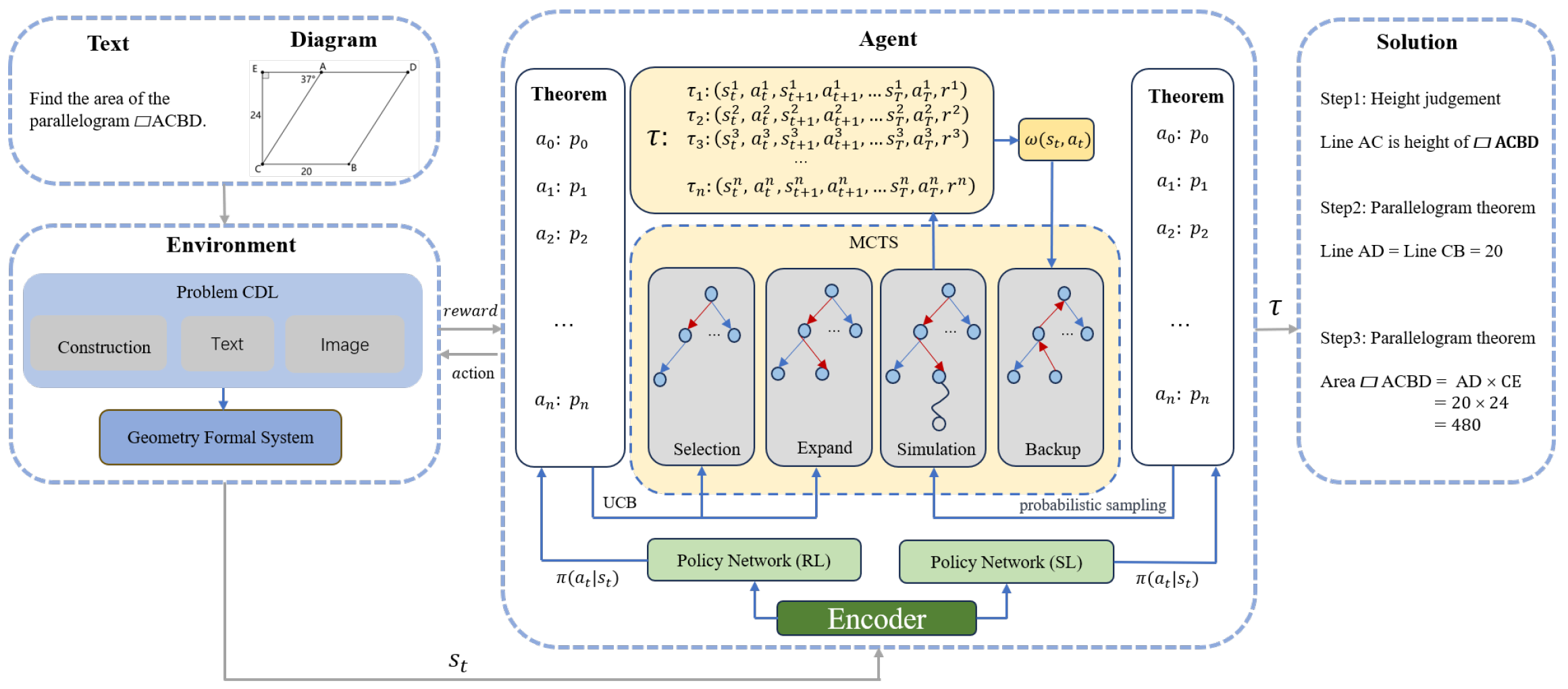
Due to the data volume falling significantly short of what is required for language model training, relying solely on the policy network for theorem application is insufficient. We need to employ a policy network within the search process, where its inclusion substantially reduces the search space. Through Monte Carlo Tree Search, data collected during the exploration phase can be utilized for training the policy network, with the primary aim being to use the cumulative rewards obtained from actual exploration to inform the learning of the reinforcement learning policy network. The reinforcement learning network we use is initialized with parameters consistent with those of the policy network. As our learning objective is the probability distribution of theorems, the reinforcement learning network employs policy gradient learning during the training phase [27]. By leveraging the cumulative reward feedback obtained from Monte Carlo Tree Search [12,23], we can further reinforce the probability of making correct theorem selections. Algorithm 1 demonstrates how Monte Carlo Tree Search performs trajectory prediction. Our goal is to find parameters theta that maximize the objective function , that is, to find a policy that maximizes , where represents a trajectory from the initial state to the terminal state, is the cumulative reward garnered along this trajectory, and represents the expected cumulative reward over the multiple trajectories collected. Please refer to Equation (2) for details, where represents the theorem selection strategy. In order to prevent overfitting of the policy network, we utilize the policy network obtained through supervised learning as our theorem predictor during the simulation phase. The parameters of this predictor remain consistent with the previous generation of reinforcement learning policy networks. In the theorem selection and expansion stages, we employ the latest reinforcement learning strategy for theorem selection [28]. Refer to Figure 2 for the specific model.
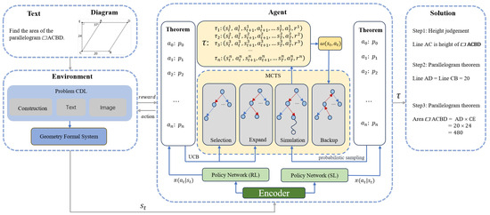
Figure 2.
The overall architecture of the FGeo-DRL model framework. (The arrow between the Agent module and the Solution module represents the final problem-solving path obtained through the Agent).
| Algorithm 1 Agent Trajectory Prediction |
|
To maximize the cumulative reward, we need to optimize the path policy to enable it to select the strategy with the maximum cumulative reward. We use policy gradient to update the policy parameters:
To implement Monte Carlo Tree Search, we need to define relevant nodes and edges. Node S is described as composed of all the condition information under the current state, while an edge is described as an executable theorem in the action space. The node information includes the number of visits for each node–action pair, the prior probability , and the cumulative reward obtained by executing the corresponding action at that node [29]. In the Monte Carlo Tree Search, we can divide it into the following four stages:
Selection: From the root node, we need to choose an optimal action to execute, and the selection of the optimal action is determined by the Upper Confidence Bound (UCB) [30]. One part of UCB depends on the average reward obtained from exploration guided by the prior probability, i.e., the average reward obtained from exploration guided by the prior probability. The other part depends on the actual number of explorations selected during exploration. This is mainly to make the exploration more comprehensive, avoiding the drawback of continuously executing actions with high prior probabilities.
Expansion: For the action selected during the selection phase, the state node resulting from its execution is expanded. This expansion involves using the policy network to predict selectable theorems and leveraging prior probabilities to provide selection preferences. Subsequently, an unexpanded action is added to the tree, creating a new node by executing action . The goal of this phase is to further explore the selected node by simulating the outcome of the game and initialize statistical information for the newly expanded node.
Simulation: During the simulation phase, it is necessary to simulate the expanded state node. We set a maximum search step and simulation count, guided by the policy network to obtain more reliable simulation results within a smaller search space. For the simulation results, if the target node is reached within the maximum search steps, a reward of 1 is returned; otherwise, a reward of 0 is returned. Through multiple simulation processes, we obtain the average score for the expanded node.
Backup: For the reward scores and visit counts obtained during the simulation phase, we need to conduct backpropagation. Through backpropagation, we feed the simulation results back to the search tree to update the cumulative rewards , thereby influencing future theorem selections.
5. Experiments
5.1. Training Method
5.1.1. Policy Network Datasets
In the initial phase of the project, we need to train a policy network for guiding theorem prediction. This involves processing an annotated dataset containing 6981 geometry problems [9]. We partition this dataset into state–action pairs and delve into annotated theorems through a reinforcement learning environment. By referring to the ground truth answers, we can capture the states obtained at each step of theorem execution and the specific theorem applied . This process not only helps establish the mapping between problems and actions but also provides crucial information for subsequent learning and optimization. Finally, we categorized the 6981 questions based on question types and difficulty levels. We divided them into training, testing, and validation sets in a ratio of 0.7:0.15:0.15, resulting in 20,981, 4470, and 4470 state–action pairs for each set, respectively. The experimental results on the validation set are presented in Table 2.
Table 2.
The hit rate of the policy network.
Table 2 displays the hit rate performance of the policy network within different ranges. The term “Range” refers to the number of selectable theorems, while “Hit rate” means that the theorems are predicted by the policy network based on the current state, sorted by probability from high to low, and a number of theorems within the range of n are selected. If the theorem within this range matches the theorem manually annotated in reality, then this theorem is considered to have hit the solvable theorem sequence. A range of 1 represents the direct hit rate of the prediction results, while values greater than 1 indicate the probability of the real labels falling within the range space. As the range expands from 1 to 25, a significant increase in hit rate can be observed. This method effectively measures the ability of the policy network to narrow down the search space based on 234 possible theorems from any given state.
5.1.2. Baseline
In the formalized system, we implemented several search baselines using different search strategies [9]. We compared forward search (FW) and backward search (BW) to evaluate distinct search policies [31,32]. In the BW approach, the target node serves as the initial node, and the search progresses by continuously generating subgoals and solving them to achieve the overall search objective. FW and BW employ four main strategies, including breadth-first search (BFS), which searches layer by layer from the initial node. Depth-first search (DFS) conducts recursive depth-first traversal. Random search (RS) explores by randomly selecting actions at nodes. Beam search (BS) selects k actions for execution in the node expansion phase.
For the policy network trained through supervised learning, we will utilize it as the policy network for reinforcement learning through policy gradient learning. To achieve this, we conduct Monte Carlo Tree Search on the FormalGeo7k dataset. We set the simulation phase to 30 simulations with a maximum simulation length of approximately 30 steps. While the longest theorem sequence in the FormalGeo7k dataset reaches 25 steps, the majority of theorem sequences are within 10 steps. As the execution of theorems progresses, the state conditions become increasingly complex, leading to a significant increase in the execution time of the formalized system. If the simulation step length is set too long, it may result in a substantial increase in simulation time, severely impacting the efficiency of the search. Therefore, specific parameters need to be set for searching theorem sequences with step lengths exceeding 10. Refer to Table 3 for detailed results. In Table 3, the bold text represents the best results among the Baseline for problems of different difficulty levels. You can find detailed information about the baseline at https://github.com/BitSecret/FGPS, (accessed on 2 April 2024).
Table 3.
Comparison of search accuracy between FGeo-DRL and the baseline.
5.2. Ablation Study
In this section, we conduct ablation experiments on the FormalGeo7K dataset, considering three scenarios to explore the impact of different approaches on theorem prediction.
By directly predicting theorem sequences using the policy network, we set the number of theorems applied in each instance to 1, aiming to explore the direct accuracy of the policy network. Additionally, we employ a simulated search to showcase the generalization ability of the policy network to states. At each node in the search tree, we execute the n most probable theorems as the initial states for the next node. This approach generates a substantial amount of irrelevant information to serve as a confounding factor. Consequently, it results in node states that differ from those learned by the policy network. To some extent, this demonstrates the generalization performance of the policy network.
Assessing the efficiency gained by combining regular search with policy network pruning, where we perform beam search to simulate the impact of policy network pruning [33].
Evaluating the improvement brought by the combination of Monte Carlo Tree Search and the policy network in FGeo-DRL.
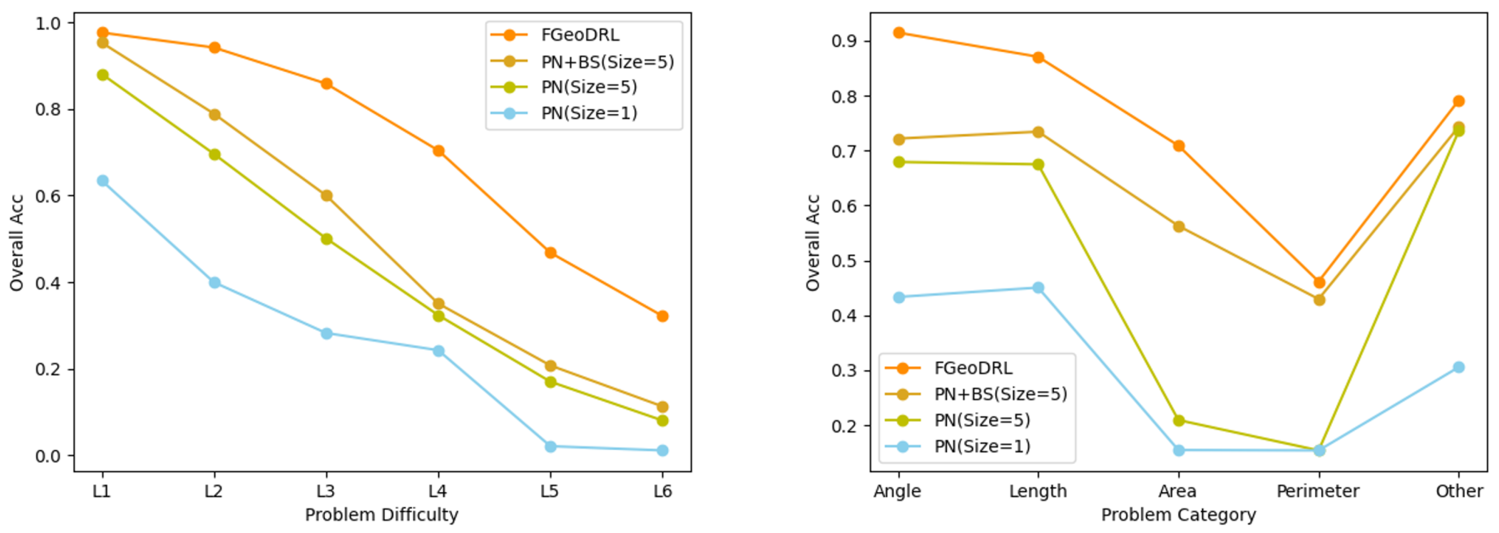
The final experimental results are presented in Table 4 and Figure 3. The “Overall Acc” represents the success rate of problem solving. In Figure 3, the horizontal axis in the left graph represents the difficulty level of the questions, while the horizontal axis in the right graph represents the types of questions.
Table 4.
Ablation study results of FormalGeo7k.
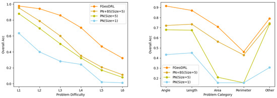
Figure 3.
Performance of different strategies on the dataset.
Regarding the experimental outcomes, it is noticeable that the assistance of Monte Carlo Tree Search significantly boosts the problem solving success rates from level to . A considerable part of this success can be attributed to the sampling feedback during the simulation phase. For problems with shorter solution sequences, there is a higher probability of reaching the solution endpoint within a finite number of steps. Upon reaching the endpoint, reward feedback facilitates the learning of problem-solving strategies by the policy network. This is particularly evident in dataset problems that involve area calculation, which, despite their lower quantity, tend to have shorter solution sequences and thus exhibit noticeably higher resolution rates compared to similar quantity problems with longer sequences, such as perimeter calculations. For problems with longer solution sequences, the performance relies more heavily on the policy network within the limited time. For problems with a greater number of questions regarding angles and lengths, their numerical advantage allows for an effective transition from short to long sequences, resulting in marked improvements in these two categories.
5.3. Discussion
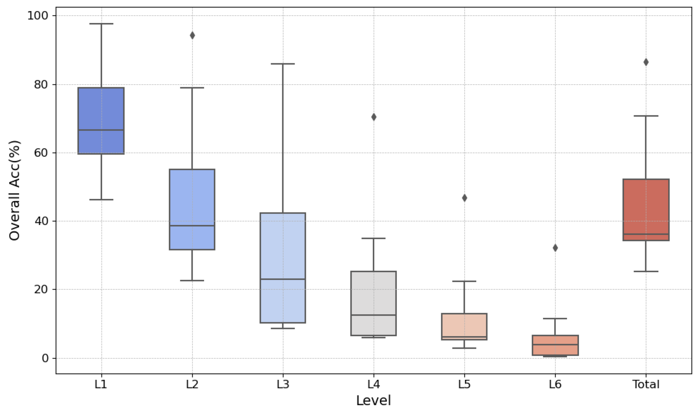
In the experimental results, we observed that FGeo-DRL significantly outperforms the traditional search methods adopted in the baseline and the direct predictions using large pre-trained language models on the FormalGeo7k dataset in every aspect. As a result, we reanalyzed the data to investigate the impact of the occurrence of extremes on our experiment [34]. By presenting the data in Table 3 through a box plot, FGeo-DRL is notably discernible as an outlier in Figure 4. This variance is particularly marked when addressing intricate problems at levels to , a phenomenon that can be ascribed to several factors. With the traditional approach, problem solving via random search leaves a choice of 234 theorems per state. The complexity of the problems scales the search space exponentially, thereby precipitously diminishing the success rate with escalating levels of difficulty. Integrating pre-trained extensive language models has led to a notable amelioration in the hit rate for theorems, as seen in Table 2. A success rate of 40.84% is attainable without any form of search by progressively predicting theorems only. The addition of Monte Carlo Tree Search along with policy gradient learning introduces an expanse of simulated searches and opportunities for refined retuning, substantially bolstering the deductive reasoning prowess and the search efficacy of FGeo-DRL in tackling complex problems.

Figure 4.
Performance of different methods at various levels.
In terms of data efficiency and learning strategies, traditional methods often struggle with sparse data environments and limited exploration capabilities [16,35]. In contrast, FGeo-DRL employs reinforcement learning, particularly Monte Carlo Tree Search, which is an effective approach to tackle the challenges of complex geometric problems. This is consistent with the observations made by Silver et al. (2016) during the development of AlphaGo [12], where Monte Carlo Tree Search played a crucial role in improving learning efficiency and decision depth. Additionally, while the random sampling theorem has been commonly employed as a solution to geometric problems, its benefit lies in reducing the time spent on manual annotation [2,22]. However, it may fall short of solving geometric problems with longer sequences of operations. Manual annotation, despite increasing labeling pressure, also represents human preference tendencies when confronted with similar issues to a certain extent. This characteristic enables the inference engine to more quickly identify breakthroughs in problem solving when faced with comparable scenarios.
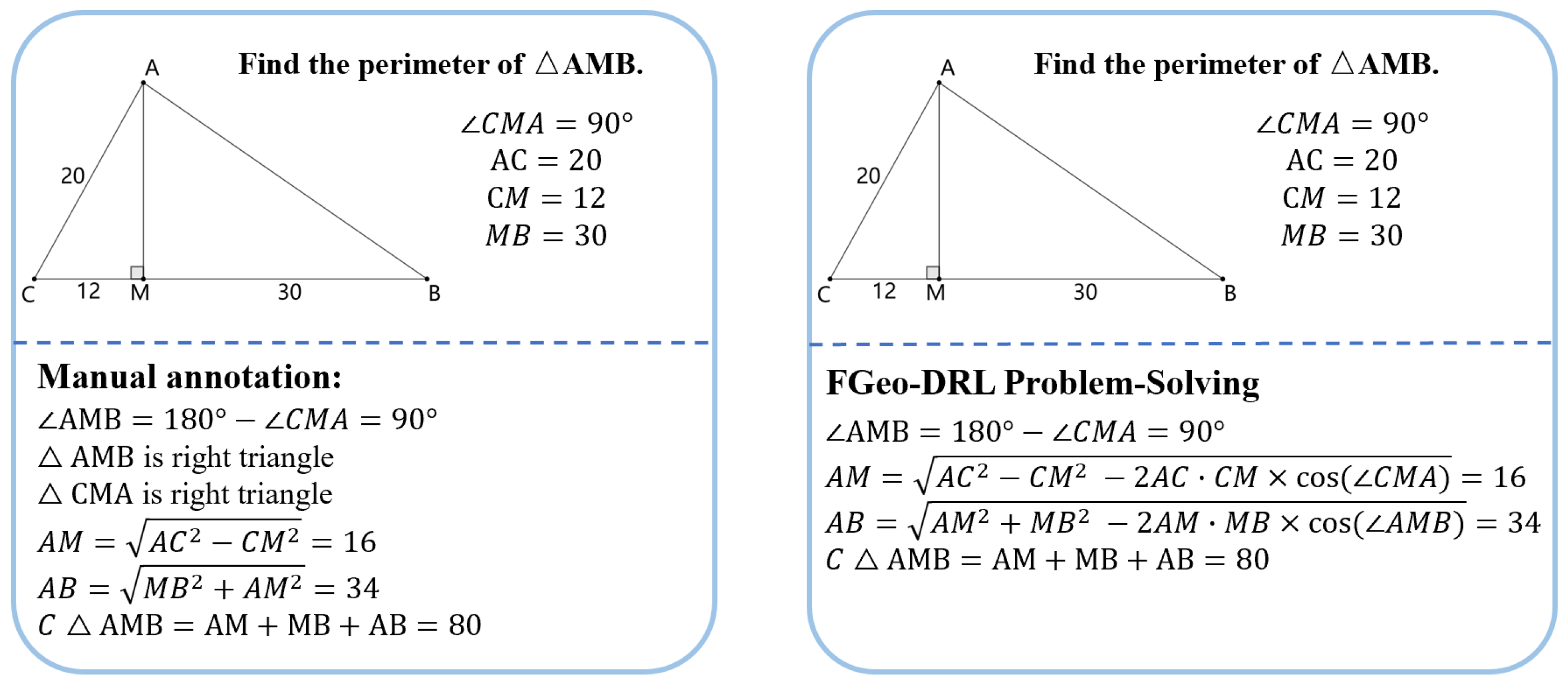
In terms of interpretability, the superiority of FGeo-DRL over past work is apparent. Contrary to past research that often failed to provide clear reasoning processes [17,36,37], FGeo-DRL demonstrates good interpretability in geometric problem reasoning. This can be attributed to the fact that a formal system offers an extensive collection of theorems, along with the reasoning tree generated through theorem reasoning. FGeo-DRL forms a theorem sequence, which extends from the initial to the terminal node, through the recording of theorems selected at each state. Furthermore, FGeo-DRL can generate problem-solving sequences distinct from those annotated manually. During the deductive reasoning process, the model offers clear probability scores for each of the 234 theorem activities at the state node and explores high-probability solutions during the Monte Carlo Tree Search process. This typically results in diverse solution paths. Under some circumstances, FGeo-DRL can even identify more succinct paths to problem resolution. For instance, as demonstrated in Figure 5, FGeo-DRL tends to employ the cosine theorem rather than the Pythagorean theorem. This method differs from those used in manual annotation and results in a more streamlined theorem exploration path.
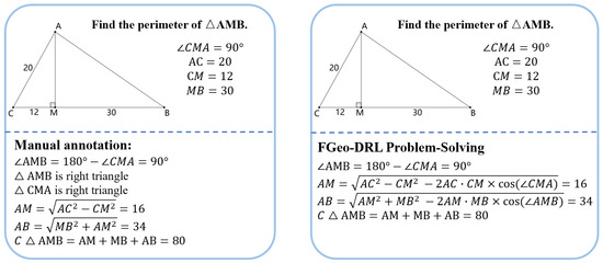
Figure 5.
The discrepancy between manual annotation and FGeo-DRL problem solving in certain geometric problems.
However, despite FGeo-DRL exhibiting strong performance on the FormalGeo7k dataset, it encounters certain limitations. Specifically, when solving problems of high difficulty, it requires an increased number of simulations and search steps to produce satisfactory outcomes, inadvertently lengthening the search duration. Furthermore, it relies on manually annotated data, including graphical details and problem descriptions, which provide essential insights and guidance throughout the geometric problem-solving process. In future work, we plan to tackle this multimodal challenge.
6. Conclusions
This paper proposes a theorem sequence prediction model, FGeo-DRL, based on a reinforcement learning framework. We implemented a pre-trained natural language model for search pruning. Additionally, we interacted Monte Carlo Tree Search with a reinforcement learning environment built through symbolic reasoning systems. By conducting searches on our proposed geometric problem dataset, FormalGeo7k, we validated the deductive reasoning of geometric problems. FGeo-DRL demonstrates superior interpretability, utilizing guided search and interactive feedback to correct experience networks. It plays a positive role in exploring both the shortest and novel solutions to geometric problems.
Author Contributions
Conceptualization, J.Z. and X.Z.; methodology, J.Z.; software, J.Z. and X.Z.; validation, J.Z.; formal analysis, Y.H. and N.Z.; data curation, J.Z., X.Z., Y.H. and N.Z.; writing—original draft preparation, J.Z.; writing—review and editing, J.Z. and T.L.; supervision, T.L.; funding acquisition, T.L. All authors have read and agreed to the published version of the manuscript.
Funding
This research was funded by the National Natural Science Foundation of China, grant number 12071282.
Data Availability Statement
The project is available at https://github.com/PersonNoName/FGeoDRL, (accessed on 2 April 2024).
Acknowledgments
Thank you for the reviewer’s valuable suggestions and comments.
Conflicts of Interest
The authors declare no conflicts of interest.
References
- Orrù, G.; Piarulli, A.; Conversano, C.; Gemignani, A. Human-like problem-solving abilities in large language models using ChatGPT. Front. Artif. Intell. 2023, 6, 1199350. [Google Scholar] [CrossRef]
- Lu, P.; Gong, R.; Jiang, S.; Qiu, L.; Huang, S.; Liang, X.; Zhu, S.C. Inter-GPS: Interpretable geometry problem solving with formal language and symbolic reasoning. arXiv 2021, arXiv:2105.04165. [Google Scholar]
- Gao, J.; Pi, R.; Zhang, J.; Ye, J.; Zhong, W.; Wang, Y.; Hong, L.; Han, J.; Xu, H.; Li, Z.; et al. G-llava: Solving geometric problem with multi-modal large language model. arXiv 2023, arXiv:2312.11370. [Google Scholar]
- Webb, T.; Holyoak, K.J.; Lu, H. Emergent analogical reasoning in large language models. Nat. Hum. Behav. 2023, 7, 1526–1541. [Google Scholar] [CrossRef]
- Sutskever, I.; Vinyals, O.; Le, Q.V. Sequence to sequence learning with neural networks. Adv. Neural Inf. Process. Syst. 2014, 27, 3104–3112. [Google Scholar]
- Nam, H.; Kim, S.; Jung, K. Number sequence prediction problems for evaluating computational powers of neural networks. In Proceedings of the AAAI Conference on Artificial Intelligence, Honolulu, HI, USA, 27 January–1 February 2019; Volume 33, pp. 4626–4633. [Google Scholar]
- Chen, J.; Tang, J.; Qin, J.; Liang, X.; Liu, L.; Xing, E.P.; Lin, L. GeoQA: A geometric question answering benchmark towards multimodal numerical reasoning. arXiv 2021, arXiv:2105.14517. [Google Scholar]
- Cao, J.; Xiao, J. An augmented benchmark dataset for geometric question answering through dual parallel text encoding. In Proceedings of the 29th International Conference on Computational Linguistics, Gyeongju, Republic of Korea, 12–17 October 2022; pp. 1511–1520. [Google Scholar]
- Zhang, X.; Zhu, N.; He, Y.; Zou, J.; Huang, Q.; Jin, X.; Guo, Y.; Mao, C.; Zhu, Z.; Yue, D.; et al. FormalGeo: The First Step Toward Human-like IMO-level Geometric Automated Reasoning. arXiv 2023, arXiv:2310.18021. [Google Scholar]
- Li, K.; Gupta, A.; Reddy, A.; Pong, V.H.; Zhou, A.; Yu, J.; Levine, S. Mural: Meta-learning uncertainty-aware rewards for outcome-driven reinforcement learning. In Proceedings of the International Conference on Machine Learning (PMLR), Virtual, 18–24 July 2021; pp. 6346–6356. [Google Scholar]
- Arjona-Medina, J.A.; Gillhofer, M.; Widrich, M.; Unterthiner, T.; Brandstetter, J.; Hochreiter, S. Rudder: Return decomposition for delayed rewards. Adv. Neural Inf. Process. Syst. 2019, 32, 13566–13577. [Google Scholar]
- Silver, D.; Huang, A.; Maddison, C.J.; Guez, A.; Sifre, L.; Van Den Driessche, G.; Schrittwieser, J.; Antonoglou, I.; Panneershelvam, V.; Lanctot, M.; et al. Mastering the game of Go with deep neural networks and tree search. Nature 2016, 529, 484–489. [Google Scholar] [CrossRef]
- Zou, J.; Zhang, X.; He, Y.; Zhu, N.; Leng, T. FGeo-DRL: Deductive Reasoning for Geometric Problems through Deep Reinforcement Learning. arXiv 2024, arXiv:2402.09051. [Google Scholar] [CrossRef]
- Gelernter, H.; Hansen, J.R.; Loveland, D.W. Empirical explorations of the geometry theorem machine. In Proceedings of the Western Joint IRE-AIEE-ACM Computer Conference, San Francisco, CA, USA, 3–5 May 1960; pp. 143–149. [Google Scholar]
- Wen-Tsun, W. Basic principles of mechanical theorem proving in elementary geometries. J. Autom. Reason. 1986, 2, 221–252. [Google Scholar] [CrossRef]
- Chou, S.C.; Gao, X.S.; Zhang, J.Z. Automated generation of readable proofs with geometric invariants: I. Multiple and shortest proof generation. J. Autom. Reason. 1996, 17, 325–347. [Google Scholar] [CrossRef]
- Seo, M.; Hajishirzi, H.; Farhadi, A.; Etzioni, O.; Malcolm, C. Solving geometry problems: Combining text and diagram interpretation. In Proceedings of the 2015 Conference on Empirical Methods in Natural Language Processing, Lisbon, Portugal, 17–21 September 2015; pp. 1466–1476. [Google Scholar]
- Kaliszyk, C.; Urban, J.; Michalewski, H.; Olšák, M. Reinforcement learning of theorem proving. Adv. Neural Inf. Process. Syst. 2018, 31, 8822–8833. [Google Scholar]
- Wu, M.; Norrish, M.; Walder, C.; Dezfouli, A. Tacticzero: Learning to prove theorems from scratch with deep reinforcement learning. Adv. Neural Inf. Process. Syst. 2021, 34, 9330–9342. [Google Scholar]
- Wu, Q.; Zhang, Q.; Huang, X. Automatic math word problem generation with topic-expression co-attention mechanism and reinforcement learning. IEEE/ACM Trans. Audio Speech Lang. Process. 2022, 30, 1061–1072. [Google Scholar] [CrossRef]
- Wang, L.; Zhang, D.; Gao, L.; Song, J.; Guo, L.; Shen, H.T. Mathdqn: Solving arithmetic word problems via deep reinforcement learning. In Proceedings of the AAAI Conference on Artificial Intelligence, New Orleans, LA, USA, 2–7 February 2018; Volume 32. [Google Scholar]
- Peng, S.; Fu, D.; Liang, Y.; Gao, L.; Tang, Z. Geodrl: A self-learning framework for geometry problem solving using reinforcement learning in deductive reasoning. In Proceedings of the Findings of the Association for Computational Linguistics: ACL 2023, Toronto, ON, Canada, 30 June 2023; pp. 13468–13480. [Google Scholar]
- Kocsis, L.; Szepesvári, C. Bandit based Monte-Carlo planning. In Proceedings of the European Conference on Machine Learning, Berlin, Germany, 18–22 September 2006; pp. 282–293. [Google Scholar]
- Puterman, M.L. Markov Decision Processes: Discrete Stochastic Dynamic Programming; John Wiley & Sons: Hoboken, NJ, USA, 1994. [Google Scholar]
- Sanh, V.; Debut, L.; Chaumond, J.; Wolf, T. DistilBERT, a distilled version of BERT: Smaller, faster, cheaper and lighter. arXiv 2019, arXiv:1910.01108. [Google Scholar]
- Devlin, J.; Chang, M.W.; Lee, K.; Toutanova, K. Bert: Pre-training of deep bidirectional transformers for language understanding. arXiv 2018, arXiv:1810.04805. [Google Scholar]
- Sutton, R.S.; McAllester, D.; Singh, S.; Mansour, Y. Policy gradient methods for reinforcement learning with function approximation. Adv. Neural Inf. Process. Syst. 1999, 12, 1057–1063. [Google Scholar]
- Van Hasselt, H.; Guez, A.; Silver, D. Deep reinforcement learning with double q-learning. In Proceedings of the AAAI Conference on Artificial Intelligence, Phoenix, AR, USA, 12–17 February 2016; Volume 30. [Google Scholar]
- Schulman, J.; Moritz, P.; Levine, S.; Jordan, M.; Abbeel, P. High-dimensional continuous control using generalized advantage estimation. arXiv 2015, arXiv:1506.02438. [Google Scholar]
- Auer, P.; Cesa-Bianchi, N.; Fischer, P. Finite-time analysis of the multiarmed bandit problem. Mach. Learn. 2002, 47, 235–256. [Google Scholar] [CrossRef]
- Nevins, A.J. Plane geometry theorem proving using forward chaining. Artif. Intell. 1975, 6, 1–23. [Google Scholar] [CrossRef]
- Gelernter, H. Realization of a geometry-theorem proving machine. In Computers & Thought; MIT Press: Cambridge, MA, USA, 1995; pp. 134–152. [Google Scholar]
- Russell, S.J.; Norvig, P. Artificial Intelligence: A Modern Approach; Pearson: London, UK, 2016. [Google Scholar]
- Jäntschi, L. Detecting extreme values with order statistics in samples from continuous distributions. Mathematics 2020, 8, 216. [Google Scholar] [CrossRef]
- Gan, W.; Yu, X.; Zhang, T.; Wang, M. Automatically proving plane geometry theorems stated by text and diagram. Int. J. Pattern Recognit. Artif. Intell. 2019, 33, 1940003. [Google Scholar] [CrossRef]
- Sachan, M.; Dubey, K.; Xing, E. From textbooks to knowledge: A case study in harvesting axiomatic knowledge from textbooks to solve geometry problems. In Proceedings of the 2017 Conference on Empirical Methods in Natural Language Processing, Copenhagen, Denmark, 7–11 September 2017; pp. 773–784. [Google Scholar]
- Sachan, M.; Xing, E. Learning to solve geometry problems from natural language demonstrations in textbooks. In Proceedings of the 6th Joint Conference on Lexical and Computational Semantics (* SEM 2017), Vancouver, Canada, 3–4 August 2017; pp. 251–261. [Google Scholar]
Disclaimer/Publisher’s Note: The statements, opinions and data contained in all publications are solely those of the individual author(s) and contributor(s) and not of MDPI and/or the editor(s). MDPI and/or the editor(s) disclaim responsibility for any injury to people or property resulting from any ideas, methods, instructions or products referred to in the content. |
© 2024 by the authors. Licensee MDPI, Basel, Switzerland. This article is an open access article distributed under the terms and conditions of the Creative Commons Attribution (CC BY) license (https://creativecommons.org/licenses/by/4.0/).