Numerical Analysis of the Discrete MRLW Equation for a Nonlinear System Using the Cubic B-Spline Collocation Method

Abstract

By employing the cubic B-spline functions, a collocation approach was devised in this study to address the Modified Regularized Long Wave (MRLW) equation. Then, we derived the corresponding nonlinear system and easily solved it using Newton’s iterative approach. It was established that the cubic B-spline collocation technique exhibits unconditional stability. The dynamics of solitary waves, including their pairwise and triadic interactions, were meticulously investigated utilizing the proposed numerical method. Additionally, the transformation of the Maxwellian initial condition into solitary wave formations is presented. To validate the current work, three distinct scenarios were compared against the analytical solution and outcomes from alternative methods under both $L_2$- and $L_{\infty }$-error norms. Primarily, the key strength of the suggested scheme lies in its capacity to yield enhanced numerical resolutions when employed to solve the MRLW equation, and these conservation laws show that the solitary waves have time and space translational symmetry in the propagation process. Finally, this paper concludes with a summary of our findings.

1. Introduction

Nonlinear partial differential equations are of great importance in elucidating various phenomena in all sorts of fields. However, exact solutions are not available for all such equations. Thus, it is necessary to employ different numerical methods to explore their possible solutions.

The form of a regularized long wave (RLW) equation is as follows:

$$u_t+u_x+\delta u{u}_x-\mu u_{xxt}=0,$$

(1)

The equation, characterized by the positive parameters $\delta$ and $\mu$, was initially put forth by Peregrine [1] to illustrate the dynamics of an undular bore, according to the symmetry and conservation law of time translation. He pioneeringly employed the finite difference method to formulate the first numerical approach for solving the RLW equation. This equation specifically encompasses events characterized by slight nonlinearity and dispersion, such as the nonlinear lateral waves occurring in shallow waters, ion-acoustic and magnetohydrodynamic disturbances within plasmas, and phonon propagations in nonlinear crystalline structures. This equation’s existence and singularity were identified by Refs. [2,3] in 1973. Later, Refs. [4,5,6,7,8,9,10] and other scholars contributed to the topic by exploring its numerical resolutions from the perspectives of the finite difference and finite element method.

So far, a multitude of numerical approaches, such as finite element methods and analytical solution strategies, have been proposed for addressing the RLW equations. According to references [11,12,13,14,15], the finite difference approaches and finite element methodologies like collocation methods that utilize quadratic, cubic, and up-to-date septic B-splines have been employed to resolve the RLW equation. Indeed, the RLW equation is a special case of the generalized long wave (GRLW) equation that has the following form:

$$u_t+u_x+\delta u^p{u}_x-\mu u_{xxt}=0,$$

(2)

This equation is characterized by a positive integer $p$ in this paper. The Generalized Regularized Long Wave (GRLW) equation has attracted little attention from researchers, with Zhang [16] exploring it through a finite difference approach to addressing a Cauchy problem and Kaya [17] employing the Adomian Decomposition Method (ADM). This work, however, delves into a distinct variant of the GRLW equation known as the Modified Regularized Long Wave (MRLW) equation. Numerical resolutions for the MRLW equation have been developed using various techniques. The finite difference method was utilized in [18], while [19,20] applied collocation methods with quintic B-splines. In a separate study, Refs. [21,22,23] employed cubic B-splines for the same purpose. The cubic B-spline Galerkin finite element method was then adopted to derive numerical solutions in [24,25,26]. The authors discuss the mixed finite element method for solving a coupled wave equation in [27] and for solving a damped Boussinesq equation in [28].

In this scheme, we continue to use the cubic B-splines for the same purpose, but we focus on temporal discrete values with a half time layer, and it is found that our scheme has better accuracy and stability than that presented in [20] for three solitary waves and for Maxwellian pulse splitting in the numerical simulation, indicating that our scheme satisfies the conservation laws perfectly.

In this study, a cubic-B-spline-based collocation technique was employed to address the MRLW equation. Section 2 details the collocation approach employed for resolving this equation, while Section 3 presents an examination of the method’s linear stability. To validate its precision, analytical solutions and conservation laws are utilized in the assessment process. The dynamics of solitary waves, including their interactions and the transformation of Maxwellian initial conditions into solitary waves, are investigated through numerical simulations in Section 4. Finally, conclusions are drawn in the closing section.

2. Governing Equation and Cubic B-Spline Collocation Method

The MRLW equation is expressed as follows:

$$u_t+u_x+6u^2{u}_x-\mu u_{xxt}=0$$

(3)

Here, the notations $x$ and $t$ symbolize differentiation, with the equation subject to boundary conditions characterized by $u\to 0$ as $x\to \pm \infty$. For the scope of this research, periodic boundary conditions are adopted within the domain $a\le x\le b$ under examination.

$$\begin{array}{l}u(a,t)=u(b,t)=0,\\ u_x(a,t)=u_x(b,t)=0.\end{array}$$

(4)

The analytical solution of this equation can be written as

$$u(x,t)=\sqrt{c}\mathrm{sech}(p(x-(c+1)t-x_0)),$$

(5)

where $p=\sqrt{\frac{c}{\mu (c+1)}}$, and $x_0$ and $c$are arbitrary constants.

Partition the interval [a,b] at points by $x_j$, where

$$a=x_0<x_1<\cdots <x_N=b$$

Here, $h=x_{j+1}-x_j=\frac{b-a}{N}$, $j=0,\cdots ,N-1$. Let${\left\{B_j\right\}}_{j=-1}^{N+1}$ the knot points denoted by $x_j$; the cubic B-splines collectively constitute a foundation of functions that span across the interval [a, b]. A global approximation solution $u_N(x,t)$ is expressed in terms of the cubic B-splines and unknown time-dependent parameters as follows:

$$u_N(x,t)={\displaystyle \sum _{j=-1}^{N+1}{c}_j{B}_j}(x)$$

(6)

Here, $c_j$ denotes unforeseen time-varying entities that are to be derived through the collocation approach, considering the constraints of boundary and initial conditions.

The cubic-B spline functions are as follows.

$$B_j(x)=\frac{1}{h^3}\left\{\begin{array}{l}{(x-x_{j-2})}^3,\hspace{0.33em}\hspace{0.33em}\hspace{0.33em}\hspace{0.33em}\hspace{0.33em}\hspace{0.33em}\hspace{0.33em}\hspace{0.33em}\hspace{0.33em}\hspace{0.33em}\hspace{0.33em}\hspace{0.33em}\hspace{0.33em}\hspace{0.33em}\hspace{0.33em}\hspace{0.33em}\hspace{0.33em}\hspace{0.33em}\hspace{0.33em}\hspace{0.33em}\hspace{0.33em}\hspace{0.33em}\hspace{0.33em}\hspace{0.33em}\hspace{0.33em}\hspace{0.33em}\hspace{0.33em}\hspace{0.33em}\hspace{0.33em}\hspace{0.33em}\hspace{0.33em}\hspace{0.33em}\hspace{0.33em}\hspace{0.33em}\hspace{0.33em}\hspace{0.33em}\hspace{0.33em}\hspace{0.33em}\hspace{0.33em}\hspace{0.33em}\hspace{0.33em}\hspace{0.33em}\hspace{0.33em}\hspace{0.33em}\hspace{0.33em}\hspace{0.33em}\hspace{0.33em}\hspace{0.33em}\hspace{0.33em}\hspace{0.33em}\hspace{0.33em}x\in \left[x_{j-2},x_{j-1}\right]\hspace{0.33em},\\ h^3+3h^2(x-x_{j-1})+3h{(x-x_{j-1})}^2-3{(x-x_{j-1})}^3,\hspace{0.33em}\hspace{0.33em}\hspace{0.33em}\hspace{0.33em}\hspace{0.33em}\hspace{0.33em}\hspace{0.33em}\hspace{0.33em}\hspace{0.33em}\hspace{0.33em}\hspace{0.33em}\hspace{0.33em}\hspace{0.33em}\hspace{0.33em}\hspace{0.33em}\hspace{0.33em}\hspace{0.33em}\hspace{0.33em}\hspace{0.33em}x\in \left[x_{j-1},x_j\right]\hspace{0.33em},\\ h^3+3h^2(x_{j+1}-x)+3h{(x_{j+1}-x)}^2-3{(x_{j+1}-x)}^3,\hspace{0.33em}\hspace{0.33em}\hspace{0.33em}\hspace{0.33em}\hspace{0.33em}\hspace{0.33em}\hspace{0.33em}\hspace{0.33em}\hspace{0.33em}\hspace{0.33em}\hspace{0.33em}\hspace{0.33em}\hspace{0.33em}\hspace{0.33em}\hspace{0.33em}\hspace{0.33em}\hspace{0.33em}\hspace{0.33em}\hspace{0.33em}x\in \left[x_j,x_{j+1}\right]\hspace{0.33em},\\ {(x_{j+2}-x)}^3,\hspace{0.33em}\hspace{0.33em}\hspace{0.33em}\hspace{0.33em}\hspace{0.33em}\hspace{0.33em}\hspace{0.33em}\hspace{0.33em}\hspace{0.33em}\hspace{0.33em}\hspace{0.33em}\hspace{0.33em}\hspace{0.33em}\hspace{0.33em}\hspace{0.33em}\hspace{0.33em}\hspace{0.33em}\hspace{0.33em}\hspace{0.33em}\hspace{0.33em}\hspace{0.33em}\hspace{0.33em}\hspace{0.33em}\hspace{0.33em}\hspace{0.33em}\hspace{0.33em}\hspace{0.33em}\hspace{0.33em}\hspace{0.33em}\hspace{0.33em}\hspace{0.33em}\hspace{0.33em}\hspace{0.33em}\hspace{0.33em}\hspace{0.33em}\hspace{0.33em}\hspace{0.33em}\hspace{0.33em}\hspace{0.33em}\hspace{0.33em}\hspace{0.33em}\hspace{0.33em}\hspace{0.33em}\hspace{0.33em}\hspace{0.33em}\hspace{0.33em}\hspace{0.33em}\hspace{0.33em}\hspace{0.33em}\hspace{0.33em}\hspace{0.33em}\hspace{0.33em}x\in \left[x_{j+1},x_{j+2}\right]\hspace{0.33em},\\ 0,\hspace{0.33em}\hspace{0.33em}\hspace{0.33em}\hspace{0.33em}\hspace{0.33em}\hspace{0.33em}\hspace{0.33em}\hspace{0.33em}\hspace{0.33em}\hspace{0.33em}\hspace{0.33em}\hspace{0.33em}\hspace{0.33em}\hspace{0.33em}\hspace{0.33em}\hspace{0.33em}\hspace{0.33em}\hspace{0.33em}\hspace{0.33em}\hspace{0.33em}\hspace{0.33em}\hspace{0.33em}\hspace{0.33em}\hspace{0.33em}\hspace{0.33em}\hspace{0.33em}\hspace{0.33em}\hspace{0.33em}\hspace{0.33em}\hspace{0.33em}\hspace{0.33em}\hspace{0.33em}\hspace{0.33em}\hspace{0.33em}\hspace{0.33em}\hspace{0.33em}\hspace{0.33em}\hspace{0.33em}\hspace{0.33em}\hspace{0.33em}\hspace{0.33em}\hspace{0.33em}\hspace{0.33em}\hspace{0.33em}\hspace{0.33em}\hspace{0.33em}\hspace{0.33em}\hspace{0.33em}\hspace{0.33em}\hspace{0.33em}\hspace{0.33em}\hspace{0.33em}\hspace{0.33em}\hspace{0.33em}\hspace{0.33em}\hspace{0.33em}\hspace{0.33em}\hspace{0.33em}\hspace{0.33em}\hspace{0.33em}\mathrm{otherwise}.\end{array}\right.$$

By employing Equation (6), the estimation of nodal values $c_j$, along with the first and second derivatives $c_j^{\prime }$ and $c_j^{″}$ at the nodal points, can be readily derived.

$$\begin{array}{l}{u}_j=c_{j-1}+4c_j+c_{j+1},\\ u_j^{\prime }=\frac{3}{h}(c_{j-1}-c_{j+1}),\\ u_j^{″}=\frac{6}{h^2}(c_{j-1}-2c_j+c_{j+1}).\end{array}$$

(7)

Let us write the MRLW equation in the following form:

$$\frac{\partial (u-\mu u_{xx})}{\partial t}+u_x+6u^2{u}_x=0.$$

(8)

Following the method used by S.I. Zaki [21] to solve the the KdVB equation, we adapt his technique to derive a recursive formula for numerically resolving Equation (8), with the temporal focus set at $(n+\frac{1}{2})\Delta t$. Here, $\Delta t$ represents the time interval, and we employ a Crank–Nicholson methodology:

$${(u_t)}^{n+\frac{1}{2}}=\frac{u^{n+1}-u^n}{\Delta t},$$

(9)

$${(u)}^{n+\frac{1}{2}}=\frac{u^{n+1}+u^n}{2},$$

(10)

$${(u^2{u}_x)}^{n+\frac{1}{2}}=\frac{{(u^2{u}_x)}^{n+1}+{(u^2{u}_x)}^n}{2},$$

(11)

Here, the notations n and n + 1 denote the chronological sequence of time steps. These computations correspond to second-order precise estimations of the values occurring at the specific time instance. Then, Equation (8) becomes

$$(u^{n+1}-\mu u_{xx}^{n+1})-(u^n-\mu u_{xx}^n)+\frac{\Delta t}{2}(u_x^{n+1}+u_x^n)+3\Delta t({(u^2{u}_x)}^{n+1}+{(u^2{u}_x)}^n)=0,$$

(12)

Introducing Equation (7) into Equation (12) yields

$$\begin{array}{l}{\left\{a_j\right\}}^{n+1}-\frac{6\mu }{h^2}{\left\{b_j\right\}}^{n+1}+\frac{3\Delta t}{2h}{\left\{c_j\right\}}^{n+1}+\frac{9\Delta t}{h}({({\left\{a_j\right\}}^{n+1})}^2{\left\{c_j\right\}}^{n+1})\\ ={\left\{a_j\right\}}^n-\frac{6\mu }{h^2}{\left\{b_j\right\}}^n-\frac{3\Delta t}{2h}{\left\{c_j\right\}}^n-\frac{9\Delta t}{h}({({\left\{a_j\right\}}^n)}^2{\left\{c_j\right\}}^n),\\ j=0,1,\cdots ,N.\end{array}$$

(13)

where

$$\left\{a_j\right\}=c_{j-1}+4c_j+c_{j+1}, \left\{b_j\right\}=c_{j-1}-2c_j+c_{j+1},$$

$$\left\{c_j\right\}=c_{j-1}-c_{j+1},j=0,1,\cdots ,N.$$

The system that emerges from Equation (13) is of a nonlinear nature. It can be effectively addressed through Newton’s iterative approach, typically achieving convergence after just two iterations.

3. Linear Stability Analysis

In order to examine the equilibrium stability of Equation (13) when linearized, we employ the Von Neumann methodology. The nonlinear term $u^2{u}_x$ is linearized by using u as a constant $\sigma$. Let $c_j^n=q^n{e}^{ikjh}$; by incorporating this into Equation (13), we obtain

$$\begin{array}{l}{q}^{n+1}[(e^{ikh}+4+e^{-ikh})-\frac{6\mu }{h^2}(e^{ikh}-2+e^{-ikh})+(\frac{3\Delta t}{2h}+\frac{9\Delta t{\sigma }^2}{h})(e^{ikh}-e^{-ikh})]e^{ikjh}\\ =q^n[(e^{ikh}+4+e^{-ikh})-\frac{6\mu }{h^2}(e^{ikh}-2+e^{-ikh})-(\frac{3\Delta t}{2h}+\frac{9\Delta t{\sigma }^2}{h})(e^{ikh}-e^{-ikh})]e^{ikjh},\end{array}$$

After some manipulations, the following can be obtained:

$$q^{n+1}=\frac{[(2\cos (kh)+4)-\frac{6\mu }{h^2}(2\cos (kh)-2)-i(\frac{3\Delta t}{h}+\frac{18\Delta t{\sigma }^2}{h})\sin (kh)]}{[(2\cos (kh)+4)-\frac{6\mu }{h^2}(2\cos (kh)-2)+i(\frac{3\Delta t}{h}+\frac{18\Delta t{\sigma }^2}{h})\sin (kh)]}{q}^n,$$

The amplification factor is given by

$$e^{\alpha k}=\frac{a-ib}{a+ib},$$

(14)

where

$$a=2\cos (kh)+4-\frac{6\mu }{h^2}(2\cos (kh)-2),$$

$$b=(\frac{3\Delta t}{h}+\frac{18\Delta t{\sigma }^2}{h})\sin (kh).$$

From Equation (13), we can deduce that

$\left|e^{\alpha k}\right|=1$ for all values of k.

So, this scheme is unconditionally stable.

4. Numerical Examples and Results

Evaluating numerical methods for evolutionary equations involves validating specific characteristics; these methods must faithfully reproduce the chronological evolution of solitary wave behavior. Throughout their propagation, the solution must maintain compliance with equivalent conservation principles. The accuracy in the movement of solitary waves can be objectively measured through the calculation of both the $L_2$-error norm

$$L_2={‖u^{exact}-u_N‖}_2=\sqrt{h{\displaystyle \sum _{j=0}^N{\left|u_j^{exact}-{(u_N)}_j\right|}^2}},$$

(15)

and $L_{\infty }$-error norm

$$L_{\infty }={‖u^{exact}-u_N‖}_{\infty }=\underset{j}{\max }\left|u_j^{exact}-{(u_N)}_j\right|.$$

(16)

Equation (3) has the following conserved quantities [19]:

$$\begin{array}{l}{I}_1={\displaystyle \underset{a}{\overset{b}{\int }}udx,}\\ I_2={\displaystyle \underset{a}{\overset{b}{\int }}(u^2+\mu u_x^2)dx,}\\ I_3={\displaystyle \underset{a}{\overset{b}{\int }}(u^4-\mu u_x^2)dx.}\end{array}$$

(17)

These characteristics facilitate the assessment of numerical methods, particularly in scenarios where analytical solutions are non-existent and during the dynamics of soliton collisions.

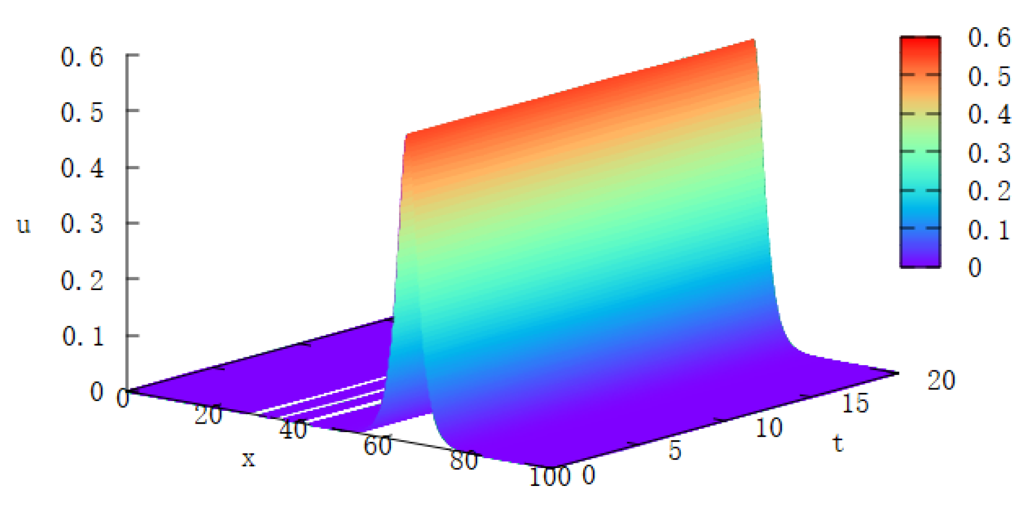
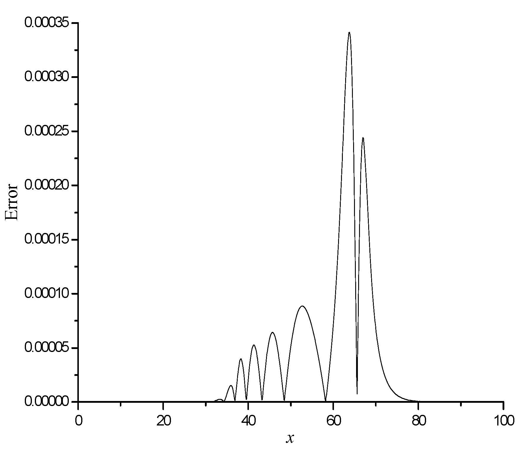
4.1. Single Solitary Waves

In case I, we set c = 0.3, $\mu$ = 1, $x_0$ = 40, h = 0.1, and $\Delta t$ = 0.01 with the following range: [0, 100]; thus, the amplitude is 0.54772. The simulations were conducted up to t = 20. The errors in $L_2$-norms and $L_{\infty }$-norms are satisfactorily small, as $L_2$-error = 7.10258 $\times$ 10⁻⁴ and $L_{\infty }$-error = 3.41575 $\times$ 10⁻⁴ at t = 20.

Table 1. Invariants and errors for a single solitary wave with c = 0.3.

Time	${\mathit{I}}_1$	${\mathit{I}}_2$	${\mathit{I}}_3$	${\mathit{L}}_2\times {10}^4$	${\mathit{L}}_{\mathit{\infty }}\times {10}^4$
0	3.58197	1.34508	0.153723	0	0
2	3.58197	1.34508	0.153723	1.67168	1.13519
4	3.58197	1.34508	0.153723	2.77610	1.63633
6	3.58197	1.34508	0.153723	3.52219	1.90878
8	3.58197	1.34508	0.153723	4.12108	2.13960
10	3.58197	1.34508	0.153723	4.65688	2.35813
12	3.58197	1.34508	0.153723	5.16261	2.57283
14	3.58197	1.34508	0.153723	5.65426	2.78427
16	3.58197	1.34508	0.153723	6.13872	2.99420
18	3.58197	1.34508	0.153723	6.62082	3.20474
20	3.58197	1.34508	0.153723	7.10258	3.41575

exhibits the findings pertaining to case II. The visual representation of the solitary wave’s progression at various temporal stages is depicted in Figure 1. A graphical comparison of the discrepancies between the analytical and computational solutions at t = 20 can be found in Figure 2, where the highest absolute error value surfaces approximately at the crest of the solitary wave.

Furthermore, when comparing the results obtained using the proposed method with the results from [19,20] in

Table 2. Errors and invariants of single solitary wave.

Schemes		Analytical	Our Scheme	Cubic B-Splin Coll-CN [20]
c = 0.3 t = 20	$I_1$	3.58197	3.58197	3.58197
	$I_2$	1.34508	1.34508	1.34508
	$I_3$	0.153723	0.153723	0.153723
	$L_2\times {10}^4$	0	7.10258	6.06885
	$L_{\infty }\times {10}^4$	0	3.41575	2.96650

, we find that when the solitary wave has an amplitude of 0.54772 (c = 0.3), our method provides the same results as the cubic B-spline collation methods [20].

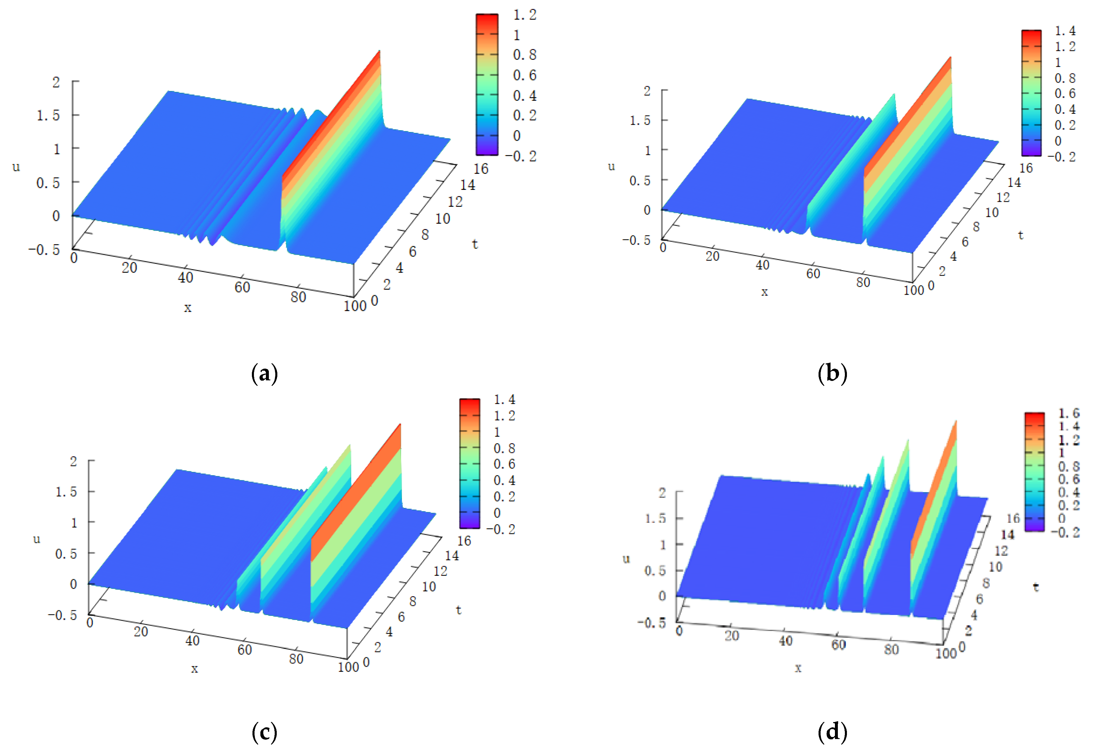
4.2. Interaction of Two Solitary Waves

The second segment of this numerical investigation explores the interaction dynamics of two solitary waves within the context of the MRLW equation. The initial scenario is established by considering a linear superposition of two distinct, amplitude-varied solitary waves that are spatially well-distinguished.

$$u(x,0)={\displaystyle \sum _{i=1}^2{A}_i}\mathrm{sech}(p_i(x-x_i)),$$

(18)

where $A_i=\sqrt{c_i}$, $p_i=\sqrt{\frac{c_i}{\mu (c_i+1)}}$, $i=1,2$.

This experiment observes the interaction of dual solitary waves, differing in amplitude yet propagating co-directionally. Upon collision, they proceed to reemerge without any alteration in their initial states. The solitary wave interaction problem was solved in the interval [0, 250] for t = 0 to t = 20 with $c_1$ = 4, $c_2$ = 1,$\mu$ = 1, $x_1$ = 25, $x_2$ = 55, a space step h = 0.2, and time step $\Delta t$ = 0.025; then, the amplitudes are in a ratio of 2:1, where$A_1$ = 2$A_2$.

Table 3. Invariants for interaction of two solitary waves.

Time	${\mathit{I}}_1$		${\mathit{I}}_2$		${\mathit{I}}_3$
	Our Scheme	Cubic B-Splin Coll-CN [20]	Our Scheme	Cubic B-Splin Coll-CN [20]	Our Scheme	CubicB-Splin Coll-CN [20]
0	11.4677	11.4677	14.6291	14.6291	22.8806	22.8806
2	11.4677	11.4677	14.6297	14.6292	22.8805	22.8807
4	11.4677	11.4677	14.6294	14.6292	22.8803	22.8807
6	11.4677	11.4677	14.6296	14.6295	22.8806	22.8806
8	11.4677	11.4677	14.6336	14.6451	22.8850	22.8454
10	11.4677	11.4677	14.6337	14.5963	22.8878	22.8913
12	11.4677	11.4677	14.6293	14.6287	22.8808	22.8814
14	11.4677	11.4677	14.6295	14.6295	22.8805	22.8807
16	11.4677	11.4677	14.6296	14.6294	22.8804	22.8808
18	11.4677	11.4677	14.6296	14.6293	22.8804	22.8809
20	11.4677	11.4677	14.6294	14.6292	22.8803	22.8809
Analytical	11.467698		14.629243		22.880466

depicts the invariants across various temporal stages. A graphical representation of the interaction among these solitary waves at distinct time levels is depicted in Figure 3.

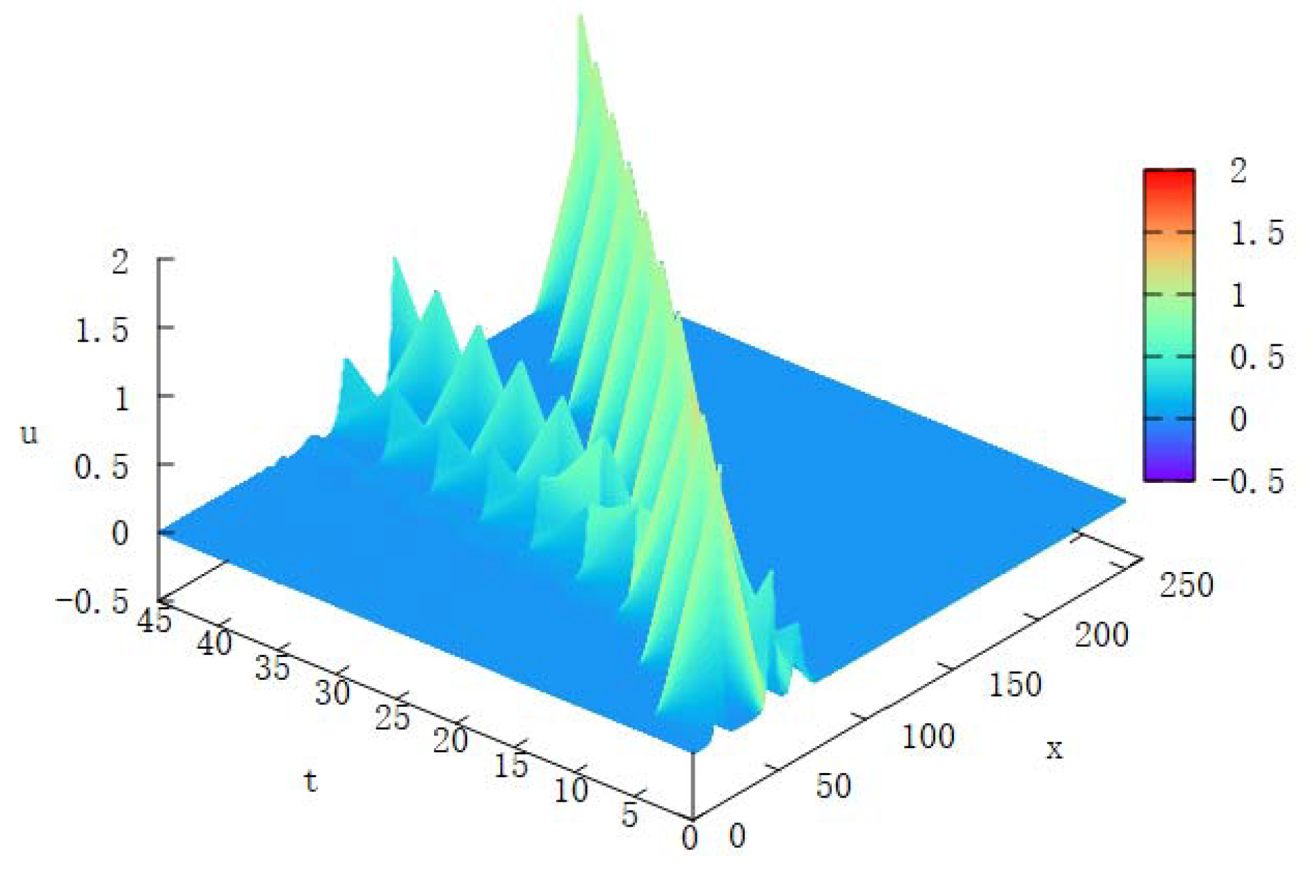
4.3. Interaction of Three Solitary Waves

This section focuses on investigating the dynamic interaction between three distinct-amplitude MRLW solitons moving co-directionally. This examination is carried out using the MRLW equation, which incorporates initial conditions that represent a linear combination of three well-spaced solitary waves, each with a unique amplitude.

$$u(x,0)={\displaystyle \sum _{i=1}^3{A}_i}\mathrm{sech}(p_i(x-x_i)),$$

(19)

where $A_i=\sqrt{c_i}$, $p_i=\sqrt{\frac{c_i}{\mu (c_i+1)}}$, $i=1,2,3$.

In our computational study, we opt for the following parameters: $c_1$ = 4, $c_2$ = 1, $c_3$ = 0.25, $\mu$ = 1, $x_1$ = 15, $x_2$ = 45, $x_3$ = 60, h = 0.2, and $\Delta t$ = 0.025, with the domain spanning from 0 to 250. The amplitude proportions are set at a ratio of 4:2:1; it is noteworthy that $A_1$ = 2$A_2$ = 4$A_3$.

Our computational study reveals that the invariants $I_1$, $I_2$, and $I_3$ for the solitary wave collisions remain constant, even with significant wave magnitudes. These observations are documented in

Table 4. Invariants for interaction of three solitary waves.

Time	${\mathit{I}}_1$		${\mathit{I}}_2$		${\mathit{I}}_3$
	Our Scheme	Cubic B-Splin Coll-CN [20]	Our Scheme	Cubic B-Splin Coll-CN [20]	Our Scheme	Cubic B-Splin Coll-CN [20]
0	14.9801	13.6891	15.8374	15.4549	23.0083	22.8816
5	14.9801	13.6891	15.8381	15.3109	23.0081	22.6939
10	14.9801	13.6891	15.8516	15.6514	23.0202	22.8388
15	14.9801	13.6891	15.8392	15.6548	23.0077	22.9347
20	14.9802	13.6891	15.8382	15.6557	23.0083	22.9330
25	14.9802	13.6892	15.8379	15.6559	23.0084	22.9336
30	14.9802	13.6894	15.8379	15.6559	23.0084	22.9348
35	14.9802	13.6913	15.8379	15.6564	23.0084	22.9343
40	14.9802	13.7015	15.8379	15.6566	23.0084	22.9335
45	14.9441	13.7043	15.8379	15.6563	23.0055	22.9303
Analytical	14.9801		15.8218		22.9923

. The intricate dynamics of these solitary waves at various temporal stages are depicted in Figure 4, extending up to t = 45.

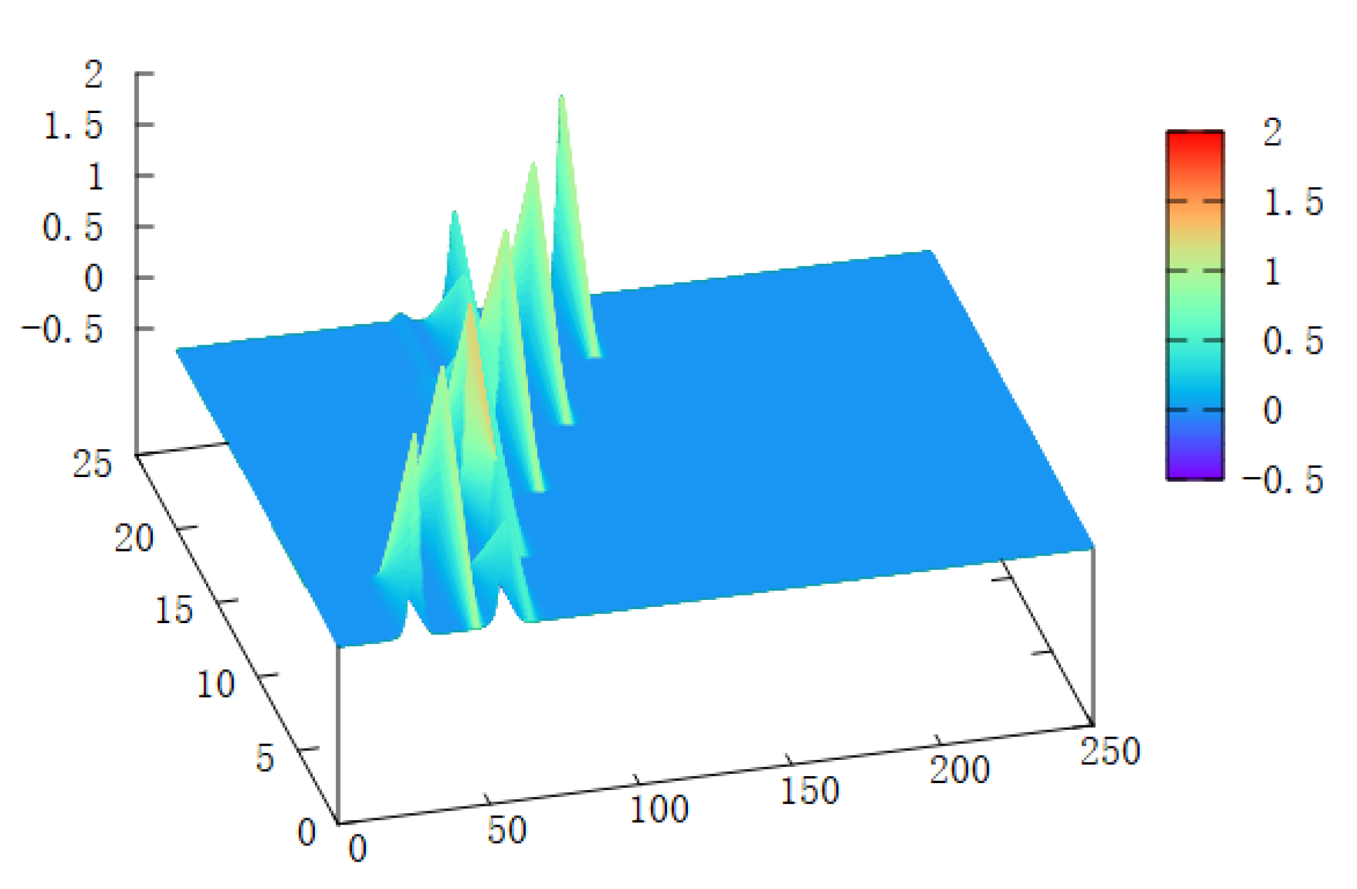
4.4. The Maxwellian Initial Condition

This section examines the progression of simulations with the adoption of a Maxwellian-based starting state,

$$u(x,0)=\exp (-{(x-40)}^2),$$

(20)

As a train of solitary waves, it is applied to the problem for different cases: (I) $\mu$ = 0.1, (II) $\mu$ = 0.04, (III) $\mu$ = 0.015, and (IV) $\mu$ = 0.01. The simulations are conducted up to t = 15. The values of the quantities$I_1$, $I_2$, and $I_3$ are given in

Table 5. Invariants of MRLW equation using the Maxwellian initial condition.

$\mathit{\mu }$	Time	${\mathit{I}}_1$	${\mathit{I}}_2$	${\mathit{I}}_3$
0.1	3	1.77247	1.37737	0.76204
	6	1.77247	1.37737	0.76204
	9	1.77247	1.37737	0.76204
	12	1.77247	1.37737	0.76204
	15	1.77247	1.37737	0.76204
0.04	3	1.77254	1.29950	0.83975
	6	1.77254	1.29951	0.83974
	9	1.77254	1.29952	0.83973
	12	1.77254	1.29952	0.83973
	15	1.77254	1.29952	0.83973
0.015	3	1.77302	1.26345	0.88107
	6	1.77302	1.26344	0.88109
	9	1.77302	1.26343	0.88100
	12	1.77302	1.26341	0.88090
	15	1.77302	1.26341	0.88087
0.01	3	1.77364	1.25554	0.89927
	6	1.77363	1.25548	0.89905
	9	1.77361	1.25525	0.89763
	12	1.77361	1.25528	0.89778
	15	1.77363	1.25551	0.89920

. However, when $\mu$ is reduced, more solitary waves formed. For case (I), only a single soliton is generated, as shown in Figure 5a, while for case (II), the Maxwellian pulse develops into a train of at least two solitary waves, as shown in Figure 5b. Similarly, Figure 5c shows that for case (III), three stable solitons are generated, and Figure 5d indicates that for case (IV), the Maxwellian initial condition has decayed into four stable solitary waves. The peaks of the well-developed wave lie on a straight line, so their velocities are linearly dependent on their amplitudes and a small oscillating tail appearing behind the last wave, as shown in Figure 5. The values of the quantities$I_1$, $I_2$, and $I_3$ for cases $\mu$ = 0.1, 0.04, 0.015, and 0.01 are given in Table 5.

Table 6. The maximum changes of invariants $I_1$, $I_2$, and $I_3$.

Computed Examples			$\Delta {\mathit{I}}_1$		$\Delta {\mathit{I}}_2$		$\Delta {\mathit{I}}_3$
			Our Scheme	Cubic B-Splin Coll-CN [20]	Our Scheme	Cubic B-Splin Coll-CN [20]	Our Scheme	Cubic B-Splin Coll-CN [20]
Single solitary waves	c = 1 (t = 10)		0	0	0.00001	0.00003	0.00001	0.00005
	c = 0.3 (t = 20)		0	0	0	0	0	0
Two solitary waves (t = 20)			0	0	0.0046	0.032	0.0075	0.0459
Three solitary waves (t = 45)			0.0361	0.0102	0.0142	0.3	0.0147	0.241
The Maxwellian initial condition (t = 15)		$\mu$ = 0.1	0	0	0	0.00005	0	0.000063
		$\mu$ = 0.04	0	0.00001	0.00002	0.00002	0.00002	0.000028
		$\mu$ = 0.015	0	0.00001	0.00004	0.00004	0.00012	0.000248
		$\mu$ = 0.01	0.00003	0.00004	0.00026	0.0004	0.00164	0.001722

presents a comparison between the cubic B-spline collocation approach [20] and our scheme according to the maximum changes $\Delta I_1$, $\Delta I_2$, and $\Delta I_3$ of invariants $I_1$, $I_2$, and $I_3$in the above computed examples. It shows that, generally, our scheme provides smaller maximum changes of the three invariants than the cubic B-spline collocation method [20], which indicates that our scheme is satisfactorily conservative.

The following is a comparison of the numerical results: In the simulation of Section 4.1 and Section 4.2, the results of the two algorithms are equivalent, but in the simulation of Section 4.3 and Section 4.4, our algorithm’s result is closer to the analytical solution, and the maximum variation of the conserved quantity is smaller, indicating that our algorithm has higher accuracy and better satisfies the conservation law of the equation.

5. Conclusions

A collocation approach employing cubic B-splines was established for generating solitary waves in the context of the MRLW equation. It was found that this approach exhibits marginal stability and surpasses other cubic B-spline collocation methods in terms of precision [19]. It was also shown in the computed examples provided in this paper that the conservation laws are substantially satisfied, where the maximum changes of three invariants in our scheme are all smaller than those in the collocation scheme [20]. We propose that these algorithms can be used to obtain numerical solutions to nonlinear differential equations. Most importantly, the use of the collocation method is especially advisable for deriving the solitary waves of nonlinear differential equations containing high-power nonlinear terms.

References

1. Peregrine, D.H. Calculations of the development of an undular bore. J. Fluid Mech. 1966, 25, 321–330. [Google Scholar] [CrossRef]
2. Bona, J.L.; Pyrant, P.J. A mathematical model for long wave generated by wave makers in nonlinear dispersive systems. Proc. Comp. Philos. Soc. 1973, 37, 91. [Google Scholar]
3. Bona, J.L.; Pritchard, W.G.; Scott, L.R. Numerical scheme for a model of nonlinear dispersive waves. J. Comput. Phys. 1985, 60, 167–176. [Google Scholar] [CrossRef]
4. Eilbeck, J.C.; McGuire, G.R. Numerical study of regularized long wave equation I: Numerical methods. J. Comput. Phys. 1975, 19, 43–57. [Google Scholar] [CrossRef]
5. Alexander, M.E.; Morris, J.H. Galerkin method for some model equation for nonlinear dispersive waves. J. Comput. Phys. 1979, 30, 428–451. [Google Scholar] [CrossRef]
6. Evans, D.J.; Raslan, K.R. The Tanh function method for solving some important nonlinear partial differential equations. Int. J. comput. Math. 2005, 82, 897–905. [Google Scholar] [CrossRef]
7. Jain, P.C.; Shankar, R.; Single, T.V. Numerical solutions of RLW equation. Commun. Numer. Meth. Eng. 1993, 9, 587–594. [Google Scholar] [CrossRef]
8. Bhardwaj, D.; Shankar, R. A computational method for regularized long wave equation. Comput. Math. Appl. 2000, 40, 1397–1404. [Google Scholar] [CrossRef]
9. Zaki, S.I. Solitary waves of the spitted RLW equation. Comput. Phys. Commun. 2001, 138, 80–91. [Google Scholar] [CrossRef]
10. Gardner, L.R.T.; Gardner, G.A.; Dogan, A. A least squares finite element scheme for the RLW equation. Commun. Numer. Meth. Eng. 1996, 12, 795–804. [Google Scholar] [CrossRef]
11. Dag, I. Least squares quadratic B-splines finite element method for the regularized long wave equation. Comput. Meth. Appl. Mech. Eng. 2000, 182, 205–215. [Google Scholar] [CrossRef]
12. Soliman, A.A.; Raslan, K.R. Collocation method using quadratic B-spline for the RLW equation. Int. J. Comput. Math. 2001, 78, 399–412. [Google Scholar] [CrossRef]
13. Dag, I.; Saka, B.; Irk, D. Application of cubic B-splins for numerical solution of the RLW equation. Appl. Math Comput. 2004, 195, 373–389. [Google Scholar]
14. Raslan, K.R. A computational method for the regularized long wave (RLW) equation. Appl. Math. Comput. 2005, 176, 1101–1118. [Google Scholar] [CrossRef]
15. Soliman, A.A.; Hussien, M.H. Collocation solution for RLW equation with septic splines. Appl. Math. Comput. 2005, 161, 623–636. [Google Scholar] [CrossRef]
16. Zhang, L. A finite difference scheme for generalized long wave equation. Appl. Math. Comput. 2005, 168, 962–972. [Google Scholar] [CrossRef]
17. Kaya, D. A numerical simulation of solitary wave solutions of the generalized regularized long wave equation. Appl. Math. Comput. 2004, 149, 833–841. [Google Scholar] [CrossRef]
18. Khalifa, A.K.; Raslan, K.R.; Alzubaidi, H.M. A finite difference scheme for the MRLW and solitary wave interactions. Appl. Math. Comput. 2007, 189, 346–354. [Google Scholar] [CrossRef]
19. Gardner, L.R.T.; Gardner, G.A.; Ayoub, F.A.; Amin, N.K. Approximations of solitary waves of the MRLW equation by B-spline finite element. Arab. J. Sci. Eng. 1997, 22, 183–193. [Google Scholar]
20. Tirmizi, I.A. A numerical technique for solution of the MRLW equation using quartic B-splines. Appl. Math. Model. 2010, 34, 4151–4160. [Google Scholar]
21. Khalifa, A.K.; Raslan, K.R.; Alzubaidi, H.M. A collocation method with B-splines for solving the MRLW equation. J. Comput. Appl. Math. 2008, 212, 406–418. [Google Scholar] [CrossRef]
22. Iqbal, A.; Abd Hamid, N.N.; Md. Ismail, A.I. Soliton solution of Schrödinger equation using cubic B-spline Galerkin method. Fluids 2019, 4, 108. [Google Scholar] [CrossRef]
23. Iqbal, A.; Abd Hamid, N.N.; Ismail, A.I.M. Cubic B-spline Galerkin method for numerical solution of the coupled nonlinear Schrödinger equation. Math. Comput. Simulat. 2020, 174, 32–44. [Google Scholar] [CrossRef]
24. Zaki, S.I. A quintic B-spline finite elements scheme for the KdVB equation. Comput. Methods Appl. Mech. Engrg. 2000, 188, 121–134. [Google Scholar] [CrossRef]
25. Karakoç, S.B.G.; Uçar, Y.; Yağmurlu, N.M. Numerical solutions of the MRLW equation by cubic B-spline Galerkin finite elements method. Kuwait J. Sci. 2015, 42, 141–159. [Google Scholar]
26. Lu, C.; Huang, W.; Qiu, J. An Adaptive moving mesh finite element solution of the Regularized Long Wave Equation. J. Sci. Comput. 2018, 74, 122–144. [Google Scholar] [CrossRef]
27. Parvizi, M.; Khodadadian, A.; Eslahchi, M.R. Analysis of Ciarlet–Raviart mixed finite element methods for solving damped Boussinesq equation. J. Comput. Appl. Math. 2020, 379, 112818. [Google Scholar] [CrossRef]
28. Parvizi, M.; Khodadadian, A.; Eslahchi, M.R. A mixed finite element method for solving coupled wave equation of Kirchhoff type with nonlinear boundary damping and memory term. Math. Methods Appl. Sci. 2021, 44, 12500–12521. [Google Scholar] [CrossRef]
Figure 1. Single solitary wave with c = 0.3.
Symmetry 16 00438 g001
Figure 2. Errors (c = 0.3) at time t = 20.
Symmetry 16 00438 g002
Figure 3. Interaction of two solitary waves.
Symmetry 16 00438 g003
Figure 4. Interaction of three solitary waves.
Symmetry 16 00438 g004
Figure 5. The Maxwellian initial condition with (a) μ = 0.1, (b) μ = 0.04, (c) μ = 0.015, and (d) μ = 0.01.
Symmetry 16 00438 g005