Bipartite (P₆,C₆)-Free Graphs: Recognition and Optimization Problems

Abstract

The canonical decomposition of a bipartite graph is a new decomposition method that involves three operators: parallel, series, and $K⨁ S$. The class of weak-bisplit graphs is the class of totally decomposable graphs with respect to these operators, and the class of bicographs is the class of totally decomposable graphs with respect to parallel and series operators. We prove in this paper that the class of bipartite $(P_6,C_6)$-free graphs is the class of bipartite graphs that are totally decomposable with respect to parallel and $K⨁S$ operators. We present a linear time recognition algorithm for $(P_6,C_6)$-free graphs that is symmetrical to the linear recognition algorithms of weak-bisplit graphs and ${star}_{\mathrm{1,2},3}$-free bipartite graphs. As a result of this algorithm, we present efficient solutions in this class of graphs for two optimization graph problems: the maximum balanced biclique problem and the maximum independent set problem.

1. Introduction

All graphs under consideration are undirected and simple. A graph $G=(V, E)$ is called bipartite if the vertex set $V$ can be partitioned into two sets: $B$, called the black vertices, and $W$, called the white vertices, such that $E\subseteq B\times W$. So, a bipartite graph will be referred to as $G=(B\cup W,E)$. This property makes bipartite graphs useful in various practical applications, including recommender systems [1], social networks [2], and information retrieval [3]. A bipartite graph $G=(B\cup W,E)$ is called complete or biclique if $E=B\times W$. A complete bipartite graph with $\left|B\right|=n$ and $\left|W\right|=m$ is referred to as $K_{n,m}$. A ${Star}_{i,j,k}$ is a tree for which there is only one vertex $v$ of degree three and three other vertices of degree one such that the distance from $v$ to those vertices are, respectively, $i, j$, and $k$. For example, $K_{\mathrm{1,3}}$ is ${Star}_{\mathrm{1,1},1}$. We can remark that every connected component in a bipartite ${Star}_{\mathrm{1,1},1}$-free graph is either a chordless path or a chordless cycle. Fouquet et al. in [4] presented a decomposition method concerning bipartite graphs, called canonical decomposition, which is based on three operators: series, parallel, and $K⨁S$. They proved that the class of graphs that are totally decomposable with respect to these three operators of decomposition is the class of bipartite ${(Star}_{\mathrm{1,2},3},P_7)$-free graphs, which is called the class of weak-bisplit graphs since it is considered as a bipartite analog of the class of split graphs. The class of weak-bisplit graphs is a natural generalization of the class of bipartite $\left(P_6,C_6\right)$-free graphs, which is a natural generalization of the class of bipartite ${Star}_{\mathrm{1,2},2}$-free graphs, studied by Lozin in [5]. Giakoumakis et. al. [6] defined the class of bicographs as a bipartite analog of the class of cographs. It is proved in [6] that the class of bicographs is exactly the class of bipartite ${(Star}_{\mathrm{1,2},3}, P_7{, Sun}_4)$-free graphs (see Figure 1) and is the class of totally decomposable graphs with respect to parallel and series decompositions. We prove in this work that the class of bipartite $\left(P_6,C_6\right)$-free graphs is the class of totally decomposable graphs with respect to parallel and $K⨁S$ decompositions. As a result of this fact, the class of bipartite $\left(P_6,C_6\right)$-free graphs can be recognized in linear time using the recognition algorithm of weak-bisplit graphs presented in [7] or the recognition algorithm of ${Star}_{\mathrm{1,2},3}$-free graphs presented in [8]. However, since these two algorithms contain several redundant cases when projected to bipartite $\left(P_6,C_6\right)$-free graphs, we propose a symmetric algorithm of these two algorithms to adapt only the class of bipartite $\left(P_6,C_6\right)$-free graphs. As a result of this adapted algorithm, we present efficient solutions in this class of graphs for two optimization graph problems: the first is the maximum balanced biclique problem, and the second is the maximum independent set problem.

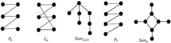
Figure 1. The configuration $P_{6,}{C}_6,{Star}_{123}$, and ${Sun}_4$.

2. Notation and Terminology

For a graph $G$, we use $V(G)$ to represent its vertex set and $E(G)$ to represent its edge set. The number $|V\left(G\right)|$is represented by $n$ and the number $|E\left(G\right)|$ is represented by $m$. If the two vertex sets $B$ and $W$ in a bipartite graph $G=(B \cup W, E)$ are both nonempty, the graph is referred to as bichromatic; otherwise, it is monochromatic. The bi-complement of bipartite graph $G=(B \cup W, E)$ is defined as ${\overline{G}}^{bip}=(B \cup W, B\times W – E)$. The set of neighbors of a vertex $v$ in $G$ is represented by $N(v)$, and the number $|N\left(v\right)|$ is referred to as the degree of $v$ and is represented by $d(v)$. A vertex $v$ is considered isolated if $d\left(v\right)=0$ and is considered universal if $d\left(v\right)=|B|$ when $v\in W$ or $d\left(v\right)=|W|$ when $v\in B$. A $2K_2$ is the complement of $C_4$. A subset $S$ of vertices of $V(G)$ is called an independent set if there is no edge between any two vertices of $S$. The sub-graph induced by a subset $X$ of vertices of $V(G)$ is represented by $G[X]$. A graph $G$ is considered $Z$-free, where $Z$ is a set of graphs, if for any subset $X\subseteq V\left(G\right), G[X]\notin Z$; that is, there is no sub-graph of $G$ isomorphic to a graph in $Z$. The decomposition of graphs according to predefined operators is a powerful method for obtaining efficient solutions to a large number of graph problems. The reader can find a survey on graph decomposition methods and their uses in [9]. In this direction, Fouquet et al. in [4] presented a decomposition method concerning bipartite graphs, which is based on three operators: decomposing a bipartite graph into connected components, decomposing the bi-complement of a bipartite graph into connected components, and decomposing a bipartite graph into $K⨁S$ components. Our recognition algorithm of bipartite ${(P}_6,C_6)$-free graphs depends mainly on this method of decomposition, so to introduce our algorithm, we need to present an overview of this method.

Definition 1 

[4]. A bipartite graph $G=(B \cup W, E)$ where $n\ge 2$ is a $K⨁S$ graph if the vertex set $V(G)$ contains an isolated vertex or there is a partition of $V(G)$ into two sets: a biclique set $K$ and an independent set $S$.

Property 1 

[4]. A bipartite graph $G=(B\cup W, E)$ with $n\ge 2$ is a $K⨁S$ graph if and only if $V(G)$ can be partitioned into two sets, $V_1$ and $V_2$, such that for every black vertex $b\in V_1$ and every white vertex $w\in V_2, bw\in E$; and for every white vertex $w\in V_1$ and every black vertex $b\in V_2, bw\notin E$.

We denote the ordered pair ${(V}_1,V_2)$ to represent the partition of the vertex set $V(G)$ of $K⨁S$ graph $G$ and we called it a $K⨁S$ partition of $G$.

Property 2 

[4]. In a bipartite graph $G=(B \cup W, E)$ that does not contain universal or isolated vertices, either $G$ is a $K⨁S$ graph or, for any partition of the black vertices $B$ or white vertices $W$ into two sets $X_1$ and $X_2$, there is an induced $2K_2$ in $G$ with vertices in both $X_1$ and $X_2$.

Corollary 1 

[4]. If a graph $G$ is not a $K⨁S$ graph, then for every vertex $v\in V(G)$, $v$ is a vertex of some $2K_2$.

Theorem 1 provides a method for decomposing a graph of type $K⨁S$.

Theorem 1 

[4]. A bipartite graph $G$ is a $K⨁S$ graph if and only if there exists a unique partition $(V_1,\dots , V_r)$ of $V(G)$, such that the following conditions hold:

• For every $i=1, \dots , r$,$V_i\ne \varnothing$.
• For every $i=1, \dots , r-1$, the sets $V_{1 }\cup \dots \cup V_i$ and $V_{i+1}\cup \dots \cup V_r$ form a $K⨁S$ partition of $G$.
• For every $i=1, \dots , r,$ the sub-graph $G[V_i]$ is not a $K⨁S$ graph.

The partition $(V_1, \dots , V_r)$ of the vertex set $V(G)$ is called the $K⨁S$ decomposition of the graph $G$, and each set $V_i$ is referred to as a $K⨁S$ component of $G$.

According to Theorem 1, the arrangement of components in a $K⨁S$ decomposition is important. Specifically, let $(V_1, \dots , V_r)$ be the $K⨁S$ decomposition of $G$; if a black vertex $b\in V_i$, then for every white vertex ${w\in V}_j$ where $j>i$, $bw\in E(G)$, and for every white vertex $w\in V_k$ where $k<i$, $bw\notin E(G)$. Similarly, if a white vertex $w\in V_i$, then for every black vertex $b\in V_j$ where $j>i$, $bw\notin E(G)$, and for every black vertex $b\in V_k$ where $k<i$, $bw\in E(G)$.

The canonical decomposition of a bipartite graph $G$ is a new decomposition method defined in [4] as follows:

• Decompose $G$ into its $K⨁S$ components; if $G$ is a $K⨁S$ graph, this decomposition is called $K⨁S$ decomposition and is denoted by $K⨁S$.
• Decompose $G$ into the connected components of $G$; if $G$ is not a connected graph, this decomposition is called parallel decomposition and is denoted by $P$.
• Decompose $G$ into the connected components of ${\overline{G}}^{bip}$; if ${\overline{G}}^{bip}$ is not a connected graph, this decomposition is called series decomposition and is denoted by $S$.
• If $G$ cannot be decomposed in $K⨁S$, parallel, or series decomposition, then $G$ is called an indecomposable graph or a prime graph.

It has been proven in [4] that no matter the order in which the operator of the decomposition is applied (series decomposition, parallel decomposition, or $K⨁S$ decomposition), the set of indecomposable graphs obtained is unique. This also creates a unique tree (up to isomorphism) associated with this decomposition known as the canonical decomposition tree. The internal nodes of the tree are labeled by the type of decomposition applied, and the leaves correspond to indecomposable graphs. Figure 2 shows an illustration of a bipartite graph and its canonical decomposition tree.

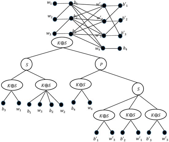
Figure 2. An example of bipartite graph $G$ and the canonical decomposition tree $T(G)$.

The canonical decomposition tree $T(G)$ of a bipartite graph $G$ resulting in an order from the $K⨁S$ decomposition, parallel decomposition, and series decomposition procedure has several properties outlined below. The terms vertex node, son, parent, and grandparent are used in their conventional sense. If $\alpha$ is an internal node, then $G[\alpha ]$ is the sub-graph induced by the set of vertex nodes having $\alpha$ as their least common grandparent.

(1)

The tree $T(G)$ consists of three types of internal nodes: parallel nodes denoted by $P$, series nodes denoted by $S$, and $K⨁S$-nodes.

(2)

Two consecutive internal nodes cannot have the same label.

(3)

An internal node $\delta$ labeled $P$ or $S$ cannot have a son that is a vertex node $v$. Otherwise, $v$ would be either an isolated or universal vertex in $G[\delta ]$. By the definition of a $K⨁S$ graph, $G[\delta ]$ would be a $K⨁S$ graph.

(4)

The parent of a vertex node is always labeled $K⨁S$ (a consequence of Property 3).

(5)

If $G$ is a bi-chromatic graph, then for any $K⨁S$ node $\delta$, $G[\delta ]$ must also be bi-chromatic. Otherwise, if there is a node $\delta$ labeled $K⨁S$ and $G[\delta ]$ is a monochromatic graph, then the parent of $\delta$, say, $\gamma$, would have isolated or universal vertices so $G[\gamma ]$ would be a $K⨁S$ graph, a contradiction with Property 2.

(6)

The sons of a $K⨁S$ node are ordered according to the $K⨁S$ decomposition.

(7)

Let $\delta$ be a $K⨁S$ node, and ${\delta }_1$ and ${\delta }_2$ are, respectively, the first and last sons of $\delta$. If the parent of $\delta$, say, $\gamma$, is a $P$-node, then ${\delta }_1$ cannot be a white vertex node and ${\delta }_2$ cannot be a black vertex node. Otherwise, by Property 1, ${\delta }_1$ and ${\delta }_2$ are isolated vertices in $G[\delta ]$; since $\gamma$ is a $P$-node, ${\delta }_1$ and ${\delta }_2$ are also isolated vertices in $G[\gamma ]$, so $\gamma$ must be a $K⨁S$ node, a contradiction with Property 2.

(8)

If the parent of a $K⨁S$-node $\delta$ is labeled $S$, and ${\delta }_1$ and ${\delta }_2$ are, respectively, the first and last sons of $\delta$, then ${\delta }_1$ cannot be a black vertex node and ${\delta }_2$ cannot be a white vertex node (similar to Property 7).

3. Recognition Algorithm of Bipartite (P₆,C₆)-Free Graphs

The following theorem is the key to our recognition algorithm for bipartite $(P_6,C_6)$-free graphs.

Theorem 2. 

A bipartite graph $G$ is ${(P}_6,C_6)$-free if and only if every connected sub-graph of $G$ is a $K⨁S$ graph.

Proof. 

Suppose that $G$ is a bipartite ${(P}_6,C_6)$-free graph. Let $H$ be a connected sub-graph of $G$ which is not a $K⨁S$ graph. By Corollary 1, $H$ contains a $2K_2$, say, $b_1{w}_1,b_2{w}_2$. Since $H$ is a connected sub-graph of $G$ and $G$ is $a (P_6,C_6)$-free graph, there is a vertex in $V(H)$ that connects $b_1{w}_1$ and $b_2{w}_2$. Suppose without a loss of generality that $b$ is a black vertex such that $b{w}_1, b{w}_2\in E(H)$. Since $H$ is not a $K⨁S$ graph, the vertex $b$ is not universal, so there is a white vertex $w$ such that $bw\notin E(H)$. Since $H$ is connected, there is a path in $H$ that connects the vertex w and the path $P_5=b_1,w_1,b,w_2,b_2$. But now, the set $\{b_1,w_1,b,w_2,b_2,w\}$ forms a $P_6$ or a $C_6$, a contradiction.

The inverse is clear since a $P_6$ or a $C_6$ is connected and contains a $2K_2$, so it is not a $K⨁S$ graph. □

Theorem 2 states that the class of bipartite ${(P}_6,C_6)$-free graphs is the smallest class closed under parallel and $K⨁S$ decomposition. So, the canonical decomposition tree of a bipartite $(P_6,C_6)$-free graph consists only of $P$-nodes or $K⨁S$-nodes. Our recognition algorithm builds a decomposition tree with $P$- or $K⨁S$-labeled internal nodes if the input graph is ${(P}_6,C_6)$-free; otherwise, it produces a failure message. This building was influenced by the cograph recognition method proposed by Corneil et al. in [10]. Moreover, this algorithm greatly simplifies two recognition algorithms when projected on bipartite ${(P}_6,C_6)$-free graphs. The first is for weak-bisplit graphs presented in [7], and the second for bipartite ${Star}_{123}$-free graphs presented in [8], where both these two algorithms need to examine more than twenty cases to confirm that the input graph is $(P_6,C_6)$-free or not, while, as we will see, our algorithm needs to examine only two cases that are presented below in Theorems 3 and 4. The algorithm begins with an empty graph and gradually adds vertices, ensuring that the resulting sub-graphs remain $(P_6,C_6)$-free. The initial bipartite graph is considered ${(P}_6,C_6)$-free if all vertices can be added successfully in this manner. The principal step of the algorithm takes into consideration the decomposition tree $T$ of a $(P_6,C_6)$-free bipartite graph $G=(B\cup W, E)$, a vertex $x\notin B\cup W$, and a set of edges denoted by $E\left(x\right)=\{xv:v\in B\cup W \mathrm{a}\mathrm{n}\mathrm{d} v\in N(x)\}$ and produces the decomposition tree $T\prime$ of the resulting graph $G\prime =(B\cup W\cup \left\{x\right\}, E\cup E\left(x\right))$ if it remains ${(P}_6,C_6)$-free or stops otherwise. The algorithm considers the connections of $x$ to other vertices in $G$ using a marking procedure. We can assume without a loss of generality that $x$ is a white vertex and the graph $G$ is a bichromatic graph.

3.1. Marking Procedure

The marking procedure, presented in Algorithm 1 and used in [10], takes into consideration the neighbors of the vertex $x$ in the graph $G$ to mark the nodes of $T$, the decomposition tree of $G$.

Algorithm 1 Marking

Input: The canonical decomposition tree $T$ of $G$ and the white vertex $x$. Output: The marking tree $T$. For every black vertex node $v$ of $T$. If $v$ is a neighbor of $x$, mark $v$ by $(t)$ if $v$ is not a neighbor of $x$, mark $v$ by $()$. Traverse $T$ on a bottom-up traversal, let $\alpha$ be an internal node of $T$: If every son of $\alpha$ which is distinct from a white vertex node is marked by $()$ then mark $\alpha$ by $()$. If there is a son of $\alpha$ marked by $(t)$ and a son marked by $()$ then mark $\alpha$ by $(p)$. If every son of $\alpha$ which is distinct from a white vertex node is marked by $(t)$ then mark $\alpha$ by $(t)$.

At the end of the marking procedure on tree $T$, a node can have three possible states: marked by $(t)$, marked by $(p)$, or marked by $()$. If a node $\delta$ is marked by$(t)$, it means that $x$ is total for $G[\delta ]$, that is, $x$ is connected to all black vertices in $G[\delta ]$. If it is marked by $(p)$, it means that $x$ is partial for $G[\delta ]$, that is, $x$ is connected to some but not all black vertices in $G[\delta ]$. If it is marked by $()$, it means that $x$ is independent of $G[\delta ]$, that is, $x$ is not connected to any black vertices in $G[\delta ]$. If a node is a vertex node, it can either be marked by $()$ or marked by $(t)$. By Theorem 2, the marking procedure focuses only on $P$-nodes and $K⨁S$-nodes, ignoring the $S$-nodes that must be unavailable. For the graph $G\prime$ to be considered bipartite and $(P_6,C_6)$-free, it must meet a necessary condition.

Lemma 1. 

If two internal nodes in the tree $T$ are marked by $(p)$, and $G\prime$ is a $(P_6,C_6)$-free bipartite graph, then one of these two nodes must be a grandparent of the other.

Proof. 

Suppose that $\alpha$ and $\beta$ are two internal nodes marked by $(p)$, then $\alpha$ and $\beta$ are partial with respect to $x$. Let $\delta$ be the least common grandparent of $\alpha$ and $\beta$. We denote $\alpha \prime$ and $\beta \prime$ to be, respectively, the son of $\delta$ containing $\alpha$ and the son of $\delta$ containing $\beta$. Since $G[\alpha ]$ and $G[\beta ]$ are sub-graphs of $G[\alpha \prime ]$ and $G[\beta \prime ]$, then $\alpha \prime$ and $\beta \prime$ are partial with respect to $x$. Assume that $\delta$ is labeled $P$, then $G[\alpha \prime ]$ and $G[\beta \prime ]$ are connected sub-graphs of $G[\delta ]$. Thus, there is an induced path $b_1,w_1, b_2$ in $G[{\alpha }^{\prime }]$ (resp. ${b\prime }_1,{w\prime }_1,{b\prime }_2$ in $G[{\beta }^{\prime }]$) such that $x$ is adjacent to $b_1$ and not adjacent to $b_2$ (resp. to ${b\prime }_1$ and not to ${b\prime }_2$). The set $\{{w\prime }_1, {b\prime }_1, x, b_1,w_1, b_2\}$ forms a $P_6$, a contradiction.

Assume that $\delta$ is labeled $K⨁S$. By Corollary 1, $\alpha \prime$ (resp. $\beta \prime$) contains a $2K_2$ that is partial with respect to $x$. Let $b_1{w}_1, b_2{w}_2$ (resp. ${b\prime }_1{w\prime }_1,{b\prime }_2{w\prime }_2$) be a $2K_2$ in $G[{\alpha }^{\prime }]$(resp. in $G[{\beta }^{\prime }]$ such that $x$ is adjacent to $b_1$ and not adjacent to $b_2$ (resp. to ${b\prime }_1$ and not to ${b\prime }_2$). Now, the set $\{w_2, b_2, {w\prime }_2, b_1, x, {b\prime }_1, {w\prime }_1\}$ forms a $P_6$, a contradiction. □

By Lemma 1, the nodes in $T$ that are marked by $(p)$ are arranged in a single path that starts from the lowest node marked by $(p)$ and goes up to the root. The lowest node marked by $(p)$ is referred to as $\alpha$. It is assumed that the conditions of Lemma 1 are met and that $\alpha$ is known. The following notations are introduced:

• Given two internal nodes $\delta$ and $\delta \prime$ such that $\delta$ is a grandparent of $\delta \prime$, the unique son of $\delta$ that contains $\delta \prime$ is denoted as $son(\delta ,\delta \prime )$.
• For an internal node $\delta$, which is either $\alpha$ or one of its grandparents, the set of sons of $\delta$ that are marked by $()$ is denoted as ${sons}^{()}(\delta )$, and the set of sons that are marked by $(t)$ is denoted as ${sons}^{(t)}(\delta )$.
• If $\delta$ has a label $K⨁S$, considering the ordering of the sons of $\delta$, the set of sons of $\delta$ marked by $(t)$ and located before $son(\delta ,\alpha )$ is denoted as ${sons}_1^{(t)}(\delta )$, and the set of sons marked by $(t)$ and located after $son(\delta ,\alpha )$ is denoted as ${sons}_2^{(t)}(\delta )$. The set of sons of $\delta$ marked by $()$ and located before $son(\delta ,\alpha )$ is denoted as ${sons}_1^{()}(\delta )$, and the set of sons marked by $()$ and located after $son(\delta ,\alpha )$ is denoted as ${sons}_2^{()}(\delta )$.

So, a node $\delta$ labeled $P$ which is a grandparent of $\alpha$ splits its sons into at most three categories: ${sons}^{\left(t\right)}(\delta )$, ${sons}^{()}(\delta )$, and $son(\delta ,\alpha )$, the son that contains $\alpha$. If $\delta$ is labeled $K⨁S$, its sons can be divided into at most five sets: $son(\delta ,\alpha )$, ${sons}_1^{(t)}(\delta )$, ${sons}_1^{()}(\delta )$, ${sons}_2^{(t)}(\delta )$, and ${sons}_2^{()}(\delta )$. Meanwhile, the sons of $\alpha$ are split into two nonempty categories: ${sons}^{()}(\alpha )$ and ${sons}^{\left(t\right)}(\alpha )$.

Definition 2. 

If $\delta$ is a grandparent of $\alpha$ in $T$, then $\delta$ is considered an incompatible $P$-node if it has at least one son marked by $(t)$ (i.e.,  ${sons}^{\left(t\right)}(\delta )\ne \varnothing )$. If $\delta$ is a $K⨁S$-node, it is considered incompatible before $\alpha$ if it has at least one son marked by $()$ located before $son(\delta ,\alpha )$ (i.e., ${sons}_1^{()}(\delta )\ne \varnothing$). If $\delta$ is a $K⨁S$-node, it is considered incompatible after $\alpha$ if it has at least one son marked by $(t)$ located after $son(\delta ,\alpha )$ (i.e., ${sons}_2^{(t)}(\alpha )\ne \varnothing$).

3.2. Building the Tree $T\prime$

We assume that the necessary condition of Lemma 1 has been verified and that all nodes that are marked by $(p)$ are known and are arranged in a single path that starts from the lowest marked node $\alpha$ and goes up to the root of $T$. To build $T\prime$, we examine the label of $\alpha$ and the presence of incompatible marked nodes. When $\alpha$ is a $K⨁S$-node, since it is the lowest node marked by $(p)$, we can divide its group of sons into a maximum of four consecutive subsets, namely, $X_1^{(t)}$, $X_2^{()}$, $X_3^{(t)}$, and $X_4$, where:

$X_1^{(t)}$ includes the first group of consecutive sons of $\alpha$ that are either a group of white vertex nodes or total with respect to $x$.

$X_2^{()}$ includes the first group of consecutive sons of $\alpha$ that are not part of $X_1^{(t)}$ and are either a group of white vertex nodes or not related to $x$.

$X_3^{(t)}$ includes the first group of consecutive sons of $\alpha$ that are not part of $X_2^{()}$ nor of $X_1^{(t)}$ and are either a group of white vertex nodes or total with respect to $x$.

$X_4$ represents the remaining sons of $\alpha$.

Note that as a result of this division of the sons of $\alpha$, when its label is $K⨁S$, $X_2^{()}$ and $X_3^{(t)}$ cannot be monochromatic graphs together.

Lemma 2. 

Assume that $\alpha$ is a $K⨁S$-node. If $G\prime$ is a bipartite $(P_6, C_6)$-free graph, then the following conditions hold:

(1)

$x$ has no neighbor in $X_4$.

(2)

If  $X_3^{(t)}$  is empty, then  ${G[X}_3^{(t)}]$ is a monochromatic graph or a complete bipartite graph.

Proof. 

Suppose that $X_4$ is not empty, otherwise, we are done. Let it show that $x$ has no neighbor in $X_4$. Since $X_4$ is not empty, then $X_3^{(t)}$ and $X_2^{()}$ are both nonempty. Let $b_4\in X_4$ such that $x$ is adjacent to $b_4$. Now, $X_4$ contains two adjacent vertices ${b\prime }_4,{w\prime }_4$ such that $x$ is not adjacent to ${b\prime }_4$; otherwise, $b_4\in X_3^{(t)}$. Let $b_2$ and $b_3$ be two black vertices of $X_2^{()}$ and $X_3^{(t)}$, respectively. By construction, there is a white vertex $w$ such that $w$ is adjacent to $b_2$ and $w$ is not adjacent to $b_3$. But now, the set $\{b_4, x, b_3, w_4, b_2,w\}$ forms a $P_6$, a contradiction. □

Now, condition 2 must be satisfied. Suppose that $X_3^{(t)}$ is not empty, then $X_2^{()}$ is also not empty.

Claim 1. 

Every element of $X_3^{(t)}$ is a vertex node.

Proof. 

Suppose that $\delta$ is an element of $X_3^{(t)}$ that is an internal node. Then $\delta$ is a $P$-node; thus, it contains a $2K_2$, say, $b_1{w}_1, b_2{w}_2$. Let $b\in X_2^{()}$, then the set $\{b,w_1, b_1, x, b_2,w_2\}$ forms a $C_6$, a contradiction. □

Claim 2. 

$X_2^{()}$contains a white vertex.

Proof. 

Suppose that $X_2^{()}$ does not contain any white vertex, then $X_3^{(t)}$ contains an element that is an internal node, a contradiction with Claim 1.

Let $b_2{,w}_2$ be two vertices of $X_2^{()}$ such that $b_2{w}_2\in E(G)$. Suppose that ${G[X}_3^{(t)}]$ is neither a monochromatic graph nor a complete bipartite graph. Then $X_3^{(t)}$ contains the vertices $b_3, {b\prime }_3,w_3$ such that $b_3$ is adjacent to $w_3$ and ${b\prime }_3$ is independent of $w_3$. Consequently, $\{{b\prime }_3, x, b_3,w_3, b_2,w_2\}$ forms a $P_6$, a contradiction. □

Theorem 3. 

Assume that there is no incompatible grandparent of $\alpha$. $G\prime$ is a bipartite $(P_6, C_6)$- free graph if and only if either:

(1)

$\alpha$ is a $P$-node; or

(2)

$\alpha$ is a $K⨁S$-node and Lemma 2 is holding.

Proof. 

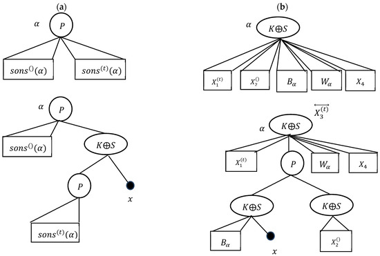
The if part of the Theorem has been proved in Lemma 2. We will describe the building of $T\prime$ for the only if part. The building of $T\prime$ when $\alpha$ is a $P$-node is described in Figure 3a. If ${sons}^{(t)}(\alpha )$ consists of a unique son, then this son will be a son of the node labeled $K⨁S$. Suppose that $\alpha$ is a $K⨁S$-node. If $X_3^{(t)}$ is empty, then we insert $x$ in $T$ as a new son of $\alpha$. The building of $T\prime$ when $G[X_3^{(t)}]$ is a monochromatic graph or a complete bipartite graph is also described in Figure 3b. In this case, if $G[X_3^{(t)}$] is a monochromatic graph, then $W_{\alpha }=\varnothing$. □

Figure 3. Building of $T\prime$ when there is no incompatible grandparent of $\alpha$.

Lemma 3. 

Assume that $G\prime$ is a bipartite $(P_6, C_6)$-free graph. If there is an incompatible grandparent $\beta$ of $\alpha$, then the following conditions hold:

(1)

$\beta$ is a $K⨁S$-incompatible node after $\alpha$.

(2)

$\beta$ is the unique incompatible grandparent of $\alpha$.

(3)

The set ${sons}_2^{(t)}(\beta )$ consists of black vertex nodes located exactly after $son(\beta ,\alpha )$.

Proof. 

Suppose that $\beta$ is an incompatible grandparent of $\mathsf{\alpha }$ of type $P$. Then there exists two adjacent vertices, $b_3,w_3$, in an element of ${sons}^{\left(t\right)}(\beta )$. Since $son(\beta ,\alpha )$ induces a connected graph, it contains an induced $P_3$, say, $b_1,w_1,b_2$, such that $b_1$ is adjacent to $x$ and $b_2$ is independent of $x$. But now, $\{x, b_1,w_1, b_2, b_3,w_3\}$ forms a $P_6$, a contradiction.

If $\beta$ is a $K⨁S$-incompatible node before α, then ${sons}_1^{()}(\beta )$ contains a black vertex $b$ independent of $x$. By Corollary 1, $son(\beta ,\alpha )$ contains a $2K_2$, say, $b_1{w}_1,b_2{w}_2$, such that $x$ is adjacent to $b_1$ and $x$ is independent of $b_2$. The set $\{x, b_1,w_1, b,w_2, b_2\}$ forms a $P_6$, a contradiction. Consequently, $\beta$ is a $K⨁S$-incompatible node after $\alpha$. Let us consider $\beta$ to be the highest incompatible grandparent of $\alpha$ and let $b\in {sons}_2^{(t)}(\beta )$. □

Claim 3. 

There is no grandparent $\delta$ of $\alpha$ containing a white vertex total for $son(\delta ,\alpha )$.

Proof. 

Let $\delta$ be a grandparent of $\alpha$ and $w$ is a white vertex of the $\delta$ total for $son(\delta ,\alpha )$. Let $b_1{w}_1,b_2{w}_2$ be an induced $2K_2$ of $son(\delta ,\alpha )$ such that $x$ is adjacent to $b_1$ and independent of $b_2$. Then the set $\{b, x, b_1,w, b_2,w_2\}$ forms a $P_6$, a contradiction.

By this claim, if $\delta$ is a $K⨁S$-incompatible node after $\alpha$, then the set ${sons}_2^{(t)}(\delta )$ consists of black vertex nodes located exactly after $son(\delta ,\alpha )$. Moreover, for every grandparent $\delta$ of $\alpha$ labeled $K⨁S$ and located between $\alpha$ and $\beta$, $son(\delta ,\alpha )$ is the last son of $\delta$; otherwise, $\delta$ contains a white vertex total for $son(\delta ,\alpha )$, a contradiction; thus, $\delta$ cannot be incompatible. Therefore, $\beta$ is the unique incompatible grandparent of $\alpha$. □

Theorem 4. 

Assume that $\beta$ is the unique $K⨁S$-incompatible grandparent after $\alpha$ and that the set ${sons}_2^{(t)}(\beta )$ consists of black vertex nodes located exactly after $son(\beta ,\alpha )$. $G\prime$ is a bipartite ${(P}_6,C_6)$-free graph if and only if one of the following conditions holds:

(1)

$\alpha$ is a $P$-node.

(2)

$\alpha$ is a $K⨁S$-node such that $X_3^{(t)}$ is an empty set.

Proof. 

Suppose that $\alpha$ is a $K⨁S$-node and let $b\in {sons}_2^{(t)}(\beta )$. Suppose that $X_3^{(t)}$ is nonempty. By Lemma 2, $G[X_3^{(t)}]$ is a monochromatic graph or a complete bipartite graph. In the two cases, $G[X_2^{()}]$ cannot be a monochromatic graph, otherwise, $X_3^{(t)}$ would be empty. Thus $X_2^{()}$ contains two adjacent vertices, $b_2,w_2$. Let $b_3$ be a black vertex of $X_3^{(t)}$. Since $G[\alpha ]$ is a connected graph, then there is a white vertex, say, $w_3$, in the last son of $\alpha$, but now $\{b, x, b_3,w_3, b_2,w_2\}$ forms a $P_6$, a contradiction.

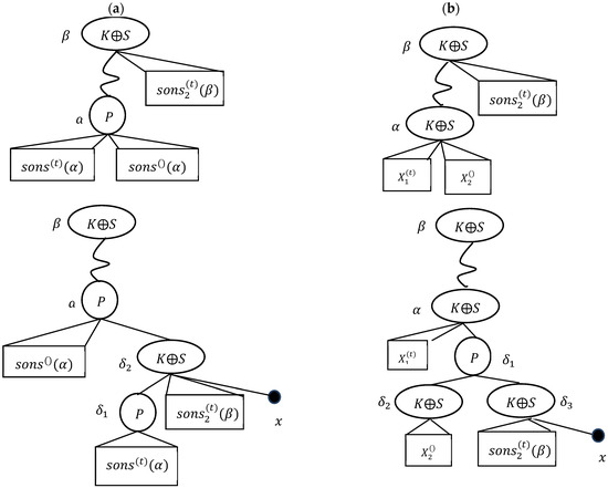
For the only if part, we describe the building of $T\prime$. When $\alpha$ is a $P$-node, the building of $T\prime$ is illustrated in Figure 4a. If the set ${sons}^{\left(t\right)}(\alpha )$ is a unique son, then this son must be labeled $K⨁S$. In this case, we delete the node ${\delta }_1$, and the element ${sons}^{\left(t\right)}(\alpha )$ will be a son of ${\delta }_2$. The building of $T\prime$ when condition 2 is satisfied is illustrated in Figure 4b. If $X_2^{()}$ is a unique son, then this son is either a node labeled $P$ or a black vertex node. In this case, we delete the node ${\delta }_2$, and the element $X_2^{()}$ will be a son of ${\delta }_1$.  □

Figure 4. Building of $T\prime$ when $\beta$, the unique $K+S$-incompatible grandparent of $\alpha$, exists.

3.3. Recognition Algorithm

The recognition algorithm of bipartite $(P_6,C_6)$-free graphs is given by Algorithm 2, whereas the procedure of the step Build-tree $(G\prime , T, head(L))$ is presented in Algorithm 3.

Algorithm 2 Recognition of bipartite $(P_6,C_6)$-free graph

Input: a bipartite graph $G=(B\cup W,E)$. Output: if $G$ is a ${(P}_6,C_6)$-free graph then the canonical decomposition tree $T(G)$, otherwise a failure message “$G$ is not $(P_6,C_6)$-free graph”. Initialization step: Let $L$ be the list of all the vertices of $G$ sorted in descending order according to their degrees. $T=$ new-vertex; $G^{\prime }=\mathrm{\varnothing }$; Build-tree $(G\prime ,T,head(L))$.

Algorithm 3 Procedure Build-tree $(G\prime , T, head(L))$

(1) Marking $(T,x)$ (2) Find the set $S=\{\delta :\delta$ is an internal node marked by $(p)\}$ (3) If $S=\mathrm{\varnothing }$ then $T=insert(x,T$) (If $x$ is independent of $T$ (resp. total for $T$) then create a new root $\delta$ of $T$ labeled $K⨁S$ such that $x$ is the left (resp. right) son of $\delta$ and the root of $T$ is the right (resp. left) son of $\delta$) (4) Else if $|S|>2$ then Exit with the message “failure”. (5) Else if $\left|S\right|=1$ then $T=insert(x,T)$ (according to Theorem 3) (6) Else if one of the two nodes of $S$ is not a grandparent of the other then Exit with the message “failure”. Else let $S=\{\alpha ,\beta \}$ and $\beta$ is the grandparent of $\alpha$ (7) If $\beta$ is a $P$-node then Exit with the message “failure”. (8) Else $T=insert(x,T)$ (according to Theorem 4) (9) $G^{\prime }=G[V(G\prime )\cup \{x\}]$; (10) If $L=\mathrm{\varnothing }$ then Exit else $L=L-\left\{x\right\}$; $x=\mathit{head}\left(L\right)$; Build-tree$(G\prime ,T,x)$

3.4. Complexity

The aim of this section is to demonstrate that recognizing a bipartite ${(P}_6,C_6)$-free graph $G$ can be accomplished in $O(n+m)$ time complexity. Since the principal step of our algorithm is the step Build-tree $(G\prime , T, x)$, we will demonstrate the linearity of our algorithm by showing that this step requires only $O(d_{G\prime }(x))$ operations, where $d_{G\prime }(x)$ is the degree of the node $x$ in $G\prime$.

It is evident that step 1 runs within $O(d_{G\prime }(x))$ time, as only a maximum of $O(d_{G\prime }(x))$ nodes are marked. Furthermore, we can assume that for every node in the tree $T$, the set of its sons that are marked by $(t)$, by $(p)$, or by $()$ has been calculated. So, finding the set $S$ also requires $O(d_{G\prime }(x))$ operations. Suppose that $S=|2|$. We can check whether one of the two nodes of $S$ is a grandparent of the other as follows: Choose an element of $S$ and start to mark the parent of this element, then mark the parent of the parent, and so on until the other element of $S$ is marked or until the root of $T$ is marked. For the last case, that is, if the root of $T$ has been marked, we repeat this process for the other element of $S$. In this manner, we can also determine the node $\alpha$, the lowest node marked by $(p)$, and the grandparent $\beta$. This process can be conducted in $O(d_{G\prime }(x))$ mark operations.

Next, we must analyze the time complexity of the function $insert (x, T)$. This requires verifying the necessary conditions in Theorem 3 or Theorem 4. Therefore, we need to compute all the required sets for building the tree $T\prime$. If $\alpha$ has the label $P$, then the computation of the set ${sons}^{\left(t\right)}(\alpha )$ and the set ${sons}^{()}(\alpha )$ is straightforward. Suppose $\alpha$ has the label $K\oplus S$. We can compute the sets $X_1^{(t)}$, $X_2^{()}$, $X_3^{(t)}$, and $X_4$ as follows: First, we compute $X_1^{(t)}$ by traversing the set of sons of $\alpha$ from left to right. In this manner, $X_1^{(t)}$ will be the first nodes that are either a set of white vertices or nodes marked by $(t)$; we continue this traversing until a son of $\alpha$ marked by $()$ has been found. The remaining sons of $\alpha$ marked by $(t)$ must belong to $X_3^{(t)}$ since $X_4$ is independent of $x$ according to Lemma 2. To compute $X_3^{(t)}$, we choose a son of $\alpha$ (let us call it $c$) from the remaining nodes marked by $(t)$ and we traverse the set of sons of $\alpha$ starting from $c$ in the left and right directions, from the left until a son of $\alpha$ marked by $()$ has been found and from the right also until a son of $\alpha$ marked by $()$ has been found or until the last son from the right has been found. We continue this traversing until every son is either a white vertex node or a node marked by $(t)$. As soon as the set $X_3^{(t)}$ has been computed, the set $X_2^{()}$ can be computed immediately. The remaining sons of $\alpha$ form the set $X_4$ which must be independent of $x$. This computation requires $O(d_{G\prime }(x))$ time complexity.

Finally, we need to determine if the node $\beta$, whose label is $K\oplus S$, is incompatible after $\alpha$ or not and check whether the set ${sons}_2^{(t)}(\beta )$ is a set of black vertex nodes located exactly after $son(\beta ,\alpha )$. These two conditions can be achieved together as follows: Since $\beta$ is known as a grandparent of $\alpha$, the son $son(\beta ,\alpha )$ is identified. Now, we can traverse the sons of $\beta$ starting from the first son located exactly after $son(\beta ,\alpha )$ and determine whether any one of these sons is a white vertex node or not. In addition, we must traverse the sons of $\beta$ starting from the first son located exactly before $son(\beta ,\alpha )$ to determine if the set ${sons}_1^{()}(\delta )$ is empty or not. This traverse also requires $O(d_{G\prime }(x))$ time complexity.

We leave it to the reader to verify that the step Build-tree $(G,T,x))$ that corresponds to insert $x$ in the tree $T$ takes a constant time in all cases.

Since testing whether $G\prime =G\cup \{x\}$ is a bipartite ${(P}_6,C_6)$-free graph or not can be performed within $O(d_{G\prime }(x))$ time complexity, it is clear that recognition of the bipartite $(P_6,C_6)$-free graph algorithm runs in $O(n+m)$ time complexity.

4. Optimization Problems

We believe that the canonical decomposition tree for a bipartite $(P_6,C_6)$-free graph can be used to find efficient solutions for several optimization graph problems because of the simple structure of this tree. In this paper, we limit ourselves to showing that the canonical decomposition tree of a bipartite $(P_6,C_6)$-free graph can be used to solve, in polynomial time, the maximum balanced biclique problem and, in linear time, the maximum independent set problem. In the concluding section of this paper, we talk about some potential uses for this result and consider it as a subject for further study.

Let $T(G)$ be the canonical decomposition tree for a bipartite $(P_6,C_6)$-free graph $G$. To present our solutions to the above two problems, we need to covert $T(G)$ to a binary tree as follows:

Visit the nodes of $T(G)$ in a depth-first search.

Let $S$ be an internal visited node, and $S_1,\dots ,S_k$ are the sons of $S$. If $k>2$, then the left son of $S$ is $S_1$, and the right son becomes a new son, $S\prime$, that has the same label as $S$ with sons $S_2,\dots ,S_k$.

4.1. Maximum Balanced Biclique Problem

A sub-graph $F=G[X\cup Y]$ of a bipartite graph $G$ is called a balanced biclique if $F$ is a biclique and $\left|X\right|=|Y|$. The balanced biclique problem is computing a balanced biclique in $G$ of maximum size. This problem is important in many different fields of study. It has numerous practical uses in very-large-scale integration (VLSI), such as the design of defect-tolerant devices [11,12], and programmable logic array folding [13]. The balanced biclique problem is NP-complete for a general bipartite graph [14], and there are very few works dedicated to obtaining an exact maximum balanced biclique, aside from the work [15] where two exact algorithms are proposed to find a maximum balanced biclique for small dense and large sparse bipartite graphs, respectively. The majority of known techniques for determining a maximum balanced biclique are heuristic algorithms (see, for example, [16,17]).

We propose in this work an $O(n^3)$ time complexity algorithm to compute a maximum balanced biclique in a bipartite ${(P}_6,C_6)$-free graph $G$ using its canonical decomposition binary tree $T(G)$. The idea of our solution is to compute all possible bicliques in $G$ that are maximal with respect to set inclusion, then find among them the one that contains a maximum balanced biclique. A biclique $F$ is maximal with respect to set inclusion if no biclique in G contains $F$. The structure of $T(G)$ when $G$ is a bipartite $(P_6,C_6)$-free graph and the definition of $K⨁S$ operation allow us to achieve this computation by a post-order traversal of $T(G)$, associating for each internal node $\alpha$ all possible maximal bicliques in $G[\alpha ]$ (with respect to set inclusion) through the two sets of maximal bicliques associated with the left son ${\alpha }_1$ and the right son ${\alpha }_2$ of $\alpha$. The set of maximal bicliques associated with ${\alpha }_1$ denoted by $L\left({\alpha }_1\right)=\{F_i^1=G\left[X_i^1\cup Y_i^1\right] :i=1,\dots ,r\}$ and the set of maximal bi-cliques associated with ${\alpha }_2$ denoted by $L\left({\alpha }_2\right)=\{F_i^2=G\left[X_i^2\cup Y_i^2\right] :i=1,\dots ,k\}$. We suppose that for every biclique $F_i^j=G\left[X_i^j\cup Y_i^j\right]$, $X_i^j$ is a set of black vertices and $Y_i^j$ is a set of white vertices. In addition, we suppose that the members of $L\left({\alpha }_1\right)$ are arranged from left to right according to their appearance in the sub-tree $T({\alpha }_1)$. Likewise, we suppose that the members of $L\left({\alpha }_2\right)$ are arranged from left to right according to their appearance in the sub-tree $T({\alpha }_2)$. This supposition is performed directly according to the arrangement of sons for every $K⨁S$-node in $T(G)$. The reader can simply verify the truth of computation used in Algorithm 4 for the set of maximal bicliques $L(\alpha )$ according to the definition of a $K⨁S$-node and the definition of a $P$-node. Figure 5 can help us to imagine this computation.

Algorithm 4 Balanced Bi-clique

$\mathrm{Input}: \mathrm{A} \mathrm{binary} \mathrm{canonical} \mathrm{decomposition} \mathrm{tree} T(G)$$\mathrm{of} \mathrm{a} \mathrm{bipartite} (P_6,C_6)$$-\mathrm{free} \mathrm{graph} G=(B\cup W, E)$. $\mathrm{Output}: \mathrm{A} \mathrm{maximal} \mathrm{balanced} \mathrm{biclique} F=G[X\cup Y]$$\mathrm{for} G$ $\mathrm{Let} \alpha$$\mathrm{be} \mathrm{a} \mathrm{node} \mathrm{on} \mathrm{a} \mathrm{post}-\mathrm{order} \mathrm{traversal} \mathrm{of} T(G)$ $\mathrm{If} \alpha$$\mathrm{is} \mathrm{a} \mathrm{black} \mathrm{vertex} \mathrm{node} b$$(\mathrm{resp}. \mathrm{a} \mathrm{white} \mathrm{vertex} \mathrm{node} w$$), \mathrm{then} L\left(\alpha \right)=\{G\left[\left\{b\right\}\cup \varnothing \right]\}$$(\mathrm{resp}. L\left(\alpha \right)=\{G\left[\varnothing \cup \left\{w\right\}\right]\}$ $\mathrm{Else} \mathrm{let} {\alpha }_1$$\mathrm{and} {\alpha }_2$$\mathrm{be} \mathrm{the} \mathrm{left} \mathrm{and} \mathrm{right} \mathrm{son} \mathrm{of} \alpha$$, \mathrm{respectively}, \mathrm{and} \mathrm{let} L\left({\alpha }_1\right)=\{F_i^1=G\left[X_i^1\cup Y_i^1\right]:i=1,\dots ,r\}$$, L\left({\alpha }_2\right)=\{F_i^2=G\left[X_i^2\cup Y_i^2\right]:i=1,\dots ,k\}$. $\mathrm{If} \alpha$$\mathrm{is} \mathrm{a} K⨁S$-node, then $\mathrm{Let} \hspace{1em}\hspace{1em}\hspace{1em}\hspace{1em}\hspace{1em}\hspace{1em}\hspace{1em}{L}_1=\{{G[(X}_1^1\cup \dots \cup X_r^1)\cup {(Y}_1^2\cup \dots \cup Y_k^2)]\}$            $L_2=\{{G[X}_i^1\cup {(Y}_i^1\cup Y_1^2\cup \dots \cup Y_k^2)]:i=1,\dots r\}$            $L_3=\{\mathrm{G}[{(X}_i^2\cup X_1^1\cup \dots \cup X_r^1)\cup Y_i^2]:i=1,\dots k\}$  If $r\ne 1$ or $k\ne 1$$, \mathrm{then} L\left(\alpha \right)=L_1\cup L_2\cup L_3$ else $L\left(\alpha \right)=L_2\cup L_3$ $\mathrm{Else}//\alpha$$\mathrm{is} \mathrm{a} P$$-\mathrm{node}//L\left(\alpha \right)=L({\alpha }_1)\cup L({\alpha }_2)$ $\mathrm{If} \alpha$$\mathrm{is} \mathrm{the} \mathrm{root} \mathrm{of} T(G)$$, \mathrm{then} \mathrm{let} L\left(\alpha \right)=\{F_i=G\left[X_i\cup Y_i\right],i=1,\dots ,s\}$ $\mathrm{Let} s_t=\mathrm{m}\mathrm{a}\mathrm{x}\{\min \left({|X}_1\left|,|Y_1|),\dots ,{\mathrm{m}\mathrm{i}\mathrm{n}(|X}_s\right|,\left|Y_s\right|\right)\}$$\mathrm{return} F_t$

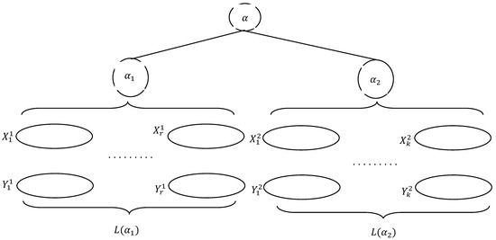
Figure 5. A node $\alpha$ and the sets of all maximal bicliques associated with its sons.

The number of bicliques computed for each internal node is at most $O(n^2)$. Since $T(G)$ contains an $O(n)$ node, the algorithm Balanced Bi-clique has a time complexity of $O(n^3)$.

4.2. Maximum Independent Set Problem

A subset $S$ of the vertex set $V(G)$ in a graph $G$ is called an independent set if any two vertices in $S$ are not adjacent. The maximum independent set problem is the task of computing an independent set in $G$ of maximum size. This problem is NP-complete for general graphs [14], but it can be solved in $O(n^{1.5}\sqrt{m/\log n})$ time complexity for a general bipartite graph [18]. This time complexity can be improved to $O(n)$ for a bipartite $(P_6,C_6)$-free graph using its canonical binary decomposition tree. The idea of our solution results from the structure of $K⨁S$ graph $G$ as follows: Let $(V_1,V_2)$ be a $K⨁S$ partition of the vertex set $V(G)$. By Property 1, every black vertex of $V_1$ is connected to every white vertex of $V_2$, and every white vertex of $V_1$ is independent of every black vertex of $V_2$. So, the maximum independent set in $G$ is either the maximum independent set in $G[V_1]$, the maximum independent set in $G[V_2]$, or the independent set formed by the union of white vertices of $G[V_1]$ and black vertices of $G[V_2]$. This remark proves the correctness of Algorithm 5. Note that if $G$ is not connected, then the maximum independent set in $G$ is equal to the union of the maximum independent sets in its connected components.

Algorithm 5 Maximum Independent Set

$\mathrm{Input}: \mathrm{A} \mathrm{binary} \mathrm{canonical} \mathrm{decomposition} \mathrm{tree} T(G)$$\mathrm{of} \mathrm{a} \mathrm{bipartite} (P_6,C_6)$$-\mathrm{free} \mathrm{graph} G=(B\cup W, E)$. $\mathrm{Output}: \mathrm{A} \mathrm{maximum} \mathrm{independent} \mathrm{set} S$$\mathrm{for} G$ $\mathrm{Let} \alpha$$\mathrm{be} \mathrm{a} \mathrm{node} \mathrm{on} \mathrm{a} \mathrm{post}-\mathrm{order} \mathrm{traversal} \mathrm{of} T(G)$. $\mathrm{If} \alpha$$\mathrm{is} \mathrm{a} \mathrm{black} \mathrm{vertex} \mathrm{node} b$$(\mathrm{resp}. \mathrm{a} \mathrm{white} \mathrm{vertex} \mathrm{node} w$), then $S\left(\alpha \right)=\{b\}$$, B\left(\alpha \right)=\{b\}$$, W\left(\alpha \right)=\varnothing$$(\mathrm{resp}. S\left(\alpha \right)=\left\{w\right\}$$, B\left(\alpha \right)=\varnothing$$, W\left(\alpha \right)=\{w\}$) $\mathrm{Else} \mathrm{let} {\alpha }_1$$\mathrm{and} {\alpha }_2$$\mathrm{be}, \mathrm{respectively}, \mathrm{the} \mathrm{left} \mathrm{and} \mathrm{right} \mathrm{son} \mathrm{of} \alpha$$\mathrm{and} \mathrm{let} S\left({\alpha }_1\right)$$\mathrm{be} \mathrm{a} \mathrm{maximum} \mathrm{independent} \mathrm{set} \mathrm{of} G[{\alpha }_1]$$\mathrm{and} S\left({\alpha }_2\right)$$\mathrm{be} \mathrm{a} \mathrm{maximum} \mathrm{independent} \mathrm{set} \mathrm{of} G[{\alpha }_2]$$; \mathrm{let} W\left({\alpha }_1\right), B\left({\alpha }_1\right)$$\mathrm{be}, \mathrm{respectively}, \mathrm{the} \mathrm{white} \mathrm{and} \mathrm{black} \mathrm{vertices} \mathrm{of} G[{\alpha }_1]$$; \mathrm{and} \mathrm{let} W\left({\alpha }_2\right), B\left({\alpha }_2\right)$$\mathrm{be}, \mathrm{respectively}, \mathrm{the} \mathrm{white} \mathrm{and} \mathrm{black} \mathrm{vertices} \mathrm{of} G[{\alpha }_2]$. $\mathrm{If} \alpha$$\mathrm{is} \mathrm{a} K⨁S$-node, then $s=\max \left\{\left|S\left({\alpha }_1\right)\right|, \left|S\left({\alpha }_2\right)\right|, \left|W\left({\alpha }_1\right)\cup B\left({\alpha }_2\right)\right|\right\}$ $S\left(\alpha \right)=S$$\mathrm{where} \left|S\right|=s$$, W\left(\alpha \right)=W({\alpha }_1)\cup W({\alpha }_2)$$\mathrm{and} B\left(\alpha \right)=B({\alpha }_1)\cup B({\alpha }_2)$ $\mathrm{else}//\alpha$$\mathrm{is} \mathrm{a} P$-node $S\left(\alpha \right)=S({\alpha }_1)\cup S({\alpha }_2)$$, W\left(\alpha \right)=W({\alpha }_1)\cup W({\alpha }_2)$$\mathrm{and} B\left(\alpha \right)=B({\alpha }_1)\cup B({\alpha }_2)$

Since $T(G)$ contains an $O(n)$ node, the algorithm’s maximum independent set has a time complexity of $O(n)$.

5. Conclusions

We have shown in this paper that bipartite $(P_6,C_6)$-free graphs can be recognized in linear time. Using this result, we solved two optimization graph problems in this class of graphs: the first is the maximum balanced biclique problem, and the second is the maximum independent set problem. An additional potential use of the canonical decomposition tree of a bipartite ${(P}_6,C_6)$-free graph is to solve the problem P| prec. $p_j=1$| C_max: Suppose there are $n$ tasks with a unit execution time, and their order is constrained by a directed acyclic graph. Additionally, there are $m$ machines of the same type. The goal is to discover a schedule that minimizes the makespan, which is the time when the final task in the graph finishes its execution. It is proved in [19] that this problem is NP-complete even if the precedence constraints form a bipartite graph of depth one. We conjecture that this problem can be solved in polynomial time for a bipartite $(P_6,C_6)$-free graph.

References

- Chakraborty, X.; Kumar, A.; Tomar, G. A survey on bipartite graph based recommender systems. Inf. Process. Manag. 2021, 58, 102536. [Google Scholar]
- Wang, R.; Wu, Y.; Hu, X.; Liu, J. Bipartite graph neural networks for social recommendation. Inf. Sci. 2021, 572, 396–409. [Google Scholar] [CrossRef]
- Biró, P.; Fleiner, T. Recent advances in matching algorithms. Eur. J. Oper. Res. 2022, 294, 745–769. [Google Scholar]
- Fouquet, J.L.; Giakoumakis, V.; Vanherpe, J.M. Bipartite graphs totally decomposable by canonical decomposition. Internat. J. Found. Comput. Sci. 1999, 10, 513–533. [Google Scholar] [CrossRef]
- Lozin, V.V. E-free bipartite graphs. Discret. Anal. Oper. Res. Ser. 2000, 7, 49–66. (In Russian) [Google Scholar]
- Giakoumakis, V.; Vanherpe, J.-M. Bi-complement reducible graphs. Adv. Appl. Math. 1997, 18, 389–402. [Google Scholar] [CrossRef][Green Version]
- Giakoumakis, V.; Vanherpe, J.M. Linear time recognition and optimization for weak bisplit graphs, bi-cographs and bipartite P6-free graphs. Int. J. Found. Comput. Sci. 2003, 14, 107–136. [Google Scholar] [CrossRef]
- Quaddoura, R. Linear time recognition of bipartite Star123-free graphs. Int. Arab. J. Inf. Technol. 2006, 3, 193–220. [Google Scholar]
- Quaddoura, R.; Mansour, K. Classical graphs decomposition and their totally decomposable graphs. IJCSNS Int. J. Comput. Sci. Netw. Secur. 2010, 10, 240–250. [Google Scholar]
- Corneil, D.G.; Perl, Y.; Stewart, L.K. A linear recognition algorithm for cographs. SIAM J. Comput. 1985, 14, 926–934. [Google Scholar] [CrossRef]
- Al-Yamani, A.; Ramsundar, S.; Pradhan, D.K. A defect tolerance scheme for nanotechnology circuits. IEEE Trans. Circuits Syst. I 2007, 54, 2402–2409. [Google Scholar] [CrossRef]
- Tahoori, M.B. Application-independent defect tolerance of reconfigurable Nano architectures. ACM J. Emerg. Technol. Comput. Syst. (JETC) 2006, 2, 197–218. [Google Scholar] [CrossRef]
- Ravi, S.; Lloyd, E.L. The complexity of near-optimal programmable logic array folding. SIAM J. Comput. 1988, 17, 696–710. [Google Scholar] [CrossRef]
- Garey, M.R.; Johnson, D.S. Computers and Intractability, A Guide to the Theory of NP-Completeness; Mathematical Series; Freeman: San Francisco, CA, USA, 1979. [Google Scholar]
- Chen, L.; Liu, C.; Zhou, R.; Xu, J.; Li, J. Efficient Exact Algorithms for Maximum Balanced Biclique Search in Bipartite Graphs. In Proceedings of the SIGMOD ’21: Proceedings of the 2021 International Conference on Management of Data, Toronto, ON, Canada, 15–18 June 2021; pp. 248–260. [Google Scholar]
- Li, M.; Hao, J.-K.; Wu, Q. General swap based multiple neighborhood adaptive search for the maximum balanced biclique problem. Comput. Oper. Res. 2020, 119, 104922. [Google Scholar] [CrossRef]
- Zhou, Y.; Hao, J.K. Tabu search with graph reduction for finding maximum balanced bicliques in bipartite graphs. Eng. Appl. Artif. Intell. 2019, 77, 86–97. [Google Scholar] [CrossRef]
- Alt, H.; Blum, N.; Mehlhorn, K.; Paul, M. Computing a maximum cardinality matching in bipartite graphs in time . Inform. Process. Lett. 1991, 37, 237–240. [Google Scholar] [CrossRef]
- Bampis, E. The Complexity of short schedules for UET bipartite graphs. RAIRO Oper. Res. 1999, 33, 367–370. [Google Scholar] [CrossRef][Green Version]
Disclaimer/Publisher’s Note: The statements, opinions and data contained in all publications are solely those of the individual author(s) and contributor(s) and not of MDPI and/or the editor(s). MDPI and/or the editor(s) disclaim responsibility for any injury to people or property resulting from any ideas, methods, instructions or products referred to in the content. |
© 2024 by the authors. Licensee MDPI, Basel, Switzerland. This article is an open access article distributed under the terms and conditions of the Creative Commons Attribution (CC BY) license (https://creativecommons.org/licenses/by/4.0/).