
YOLO-RDP: Lightweight Steel Defect Detection through Improved YOLOv7-Tiny and Model Pruning
Abstract
:1. Introduction
- Large model size and computational complexity: For deployment on edge terminal devices with limited computing power in steel plants, excessively large models and computational complexity can lead to device overload, making it impossible to detect targets;
- Steel surface defects are small targets and are easily overlooked during feature learning, leading to missed detections. Although the YOLO algorithm is known for its excellent performance and balance between accuracy and speed, detecting small targets has always been a challenge for the YOLO series of target detection algorithms.
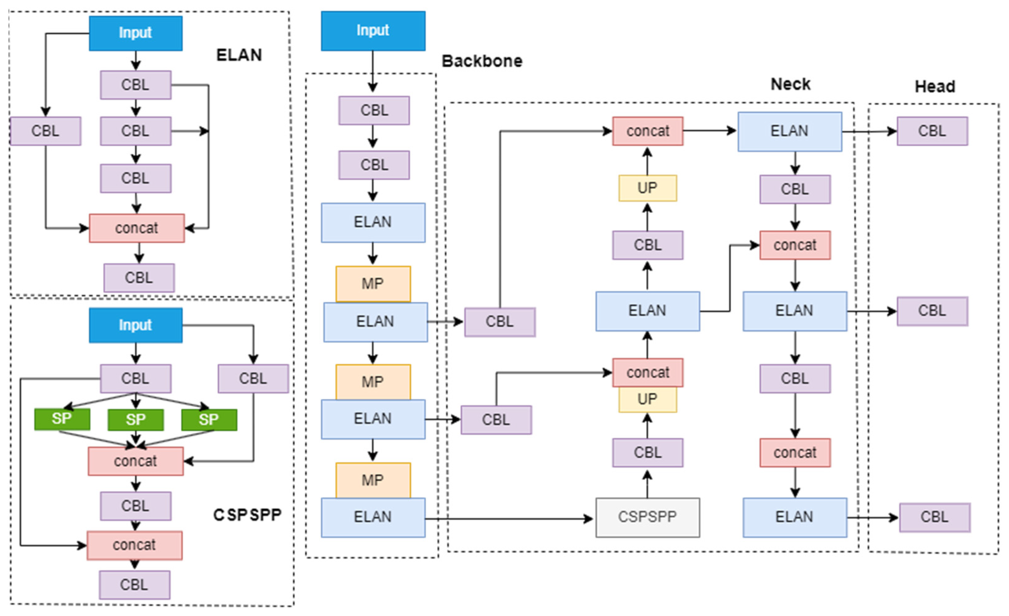
- The extensive use of ELAN networks in the Backbone, where each ELAN network consists of multiple densely connected standard convolutions, results in a complex network structure, excessive computational complexity, and a large number of parameters. Moreover, the number of network layers is too few, which is not conducive to feature extraction;
- ELAN networks are still used in the Neck section, making it easier to generate redundant features during feature aggregation;
- In the Head section, processing target position and category information together leads to excessive parameter size and computational complexity. Additionally, the lack of multi-level perception of feature information makes it difficult to improve detection performance.
- (1)
- Utilization of the lightweight network RexNet [8] for improved feature extraction in the model, reducing both parameter count and computational load;
- (2)
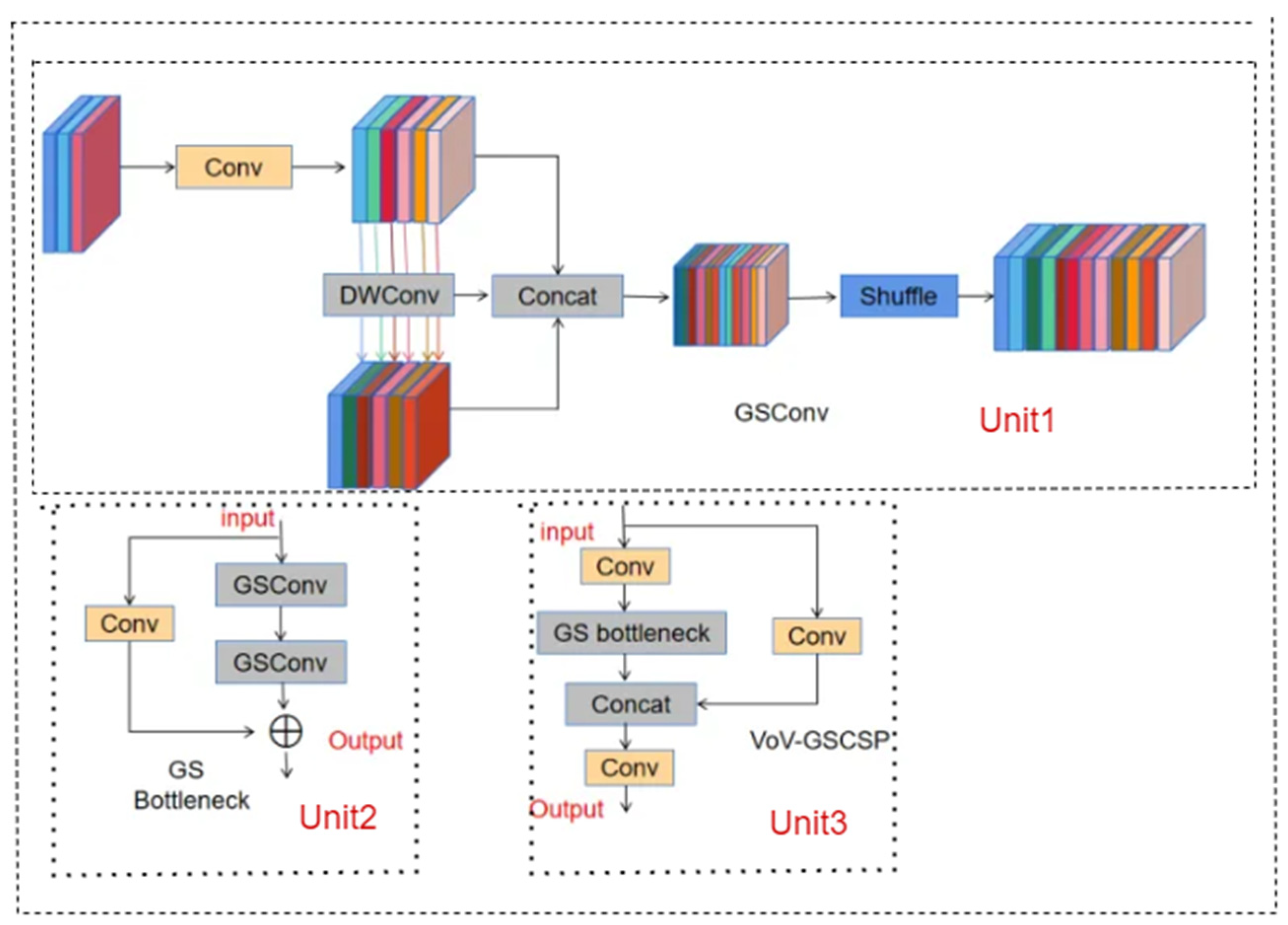
- Enhancement of the Neck section with lightweight modules GSConv [9] and VoVGSCSP [9], replacing standard convolution with GSConv to mitigate the negative impacts of DSC operations in lightweight models while leveraging DSC’s advantages. This reduces model complexity and maintains accuracy, and using VoVGSCSP instead of ELAN lowers computational complexity, fitting the limited resources of edge devices;
- (3)
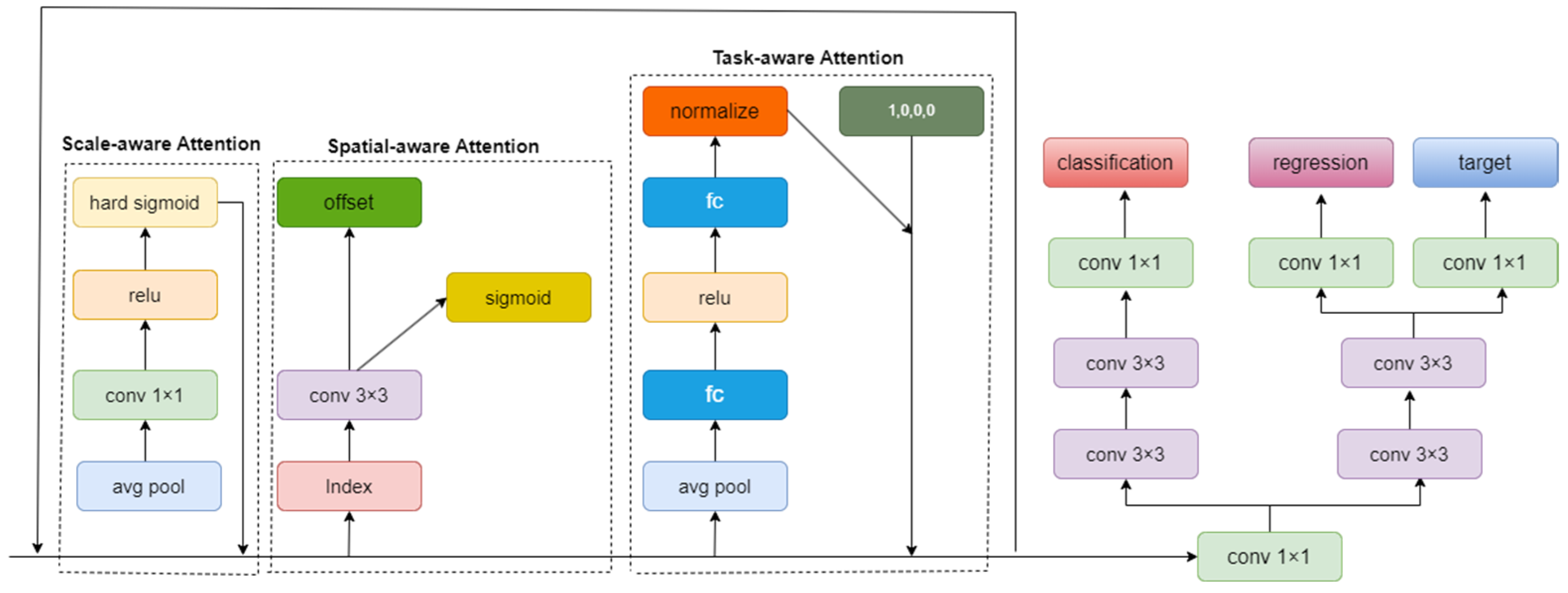
- Improvement of the original model’s detection head with an attention-enhanced detector, DdyHead, enhancing the model’s ability to recognize minor defects;
- (4)
- Further model compression through channel-level pruning algorithms without compromising accuracy. The improved YOLO-RDP model significantly enhances parameter efficiency, computational complexity, and model size, improving accuracy over the original YOLOv7-tiny model, and achieving a balance between precision and lightweighting suitable for deployment on edge devices.
2. Related Work
2.1. YOLOv7-Tiny Network Structure
2.2. Model Pruning
3. Method
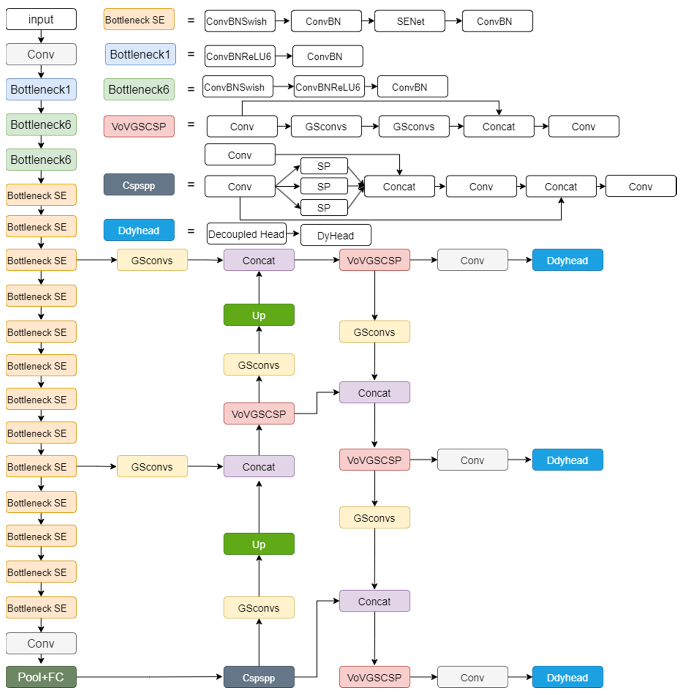
3.1. YOLO-RDP Model
3.1.1. ReXNet Lightweight Network
3.1.2. GSConv and VOV-GSCSP Lightweight Modules
3.1.3. Dual Detection Head DdyHead with a Symmetric Structure
3.2. YOLO-RDP Model Pruning
4. Experiment
4.1. Experimental Design
- (1)
- Dataset
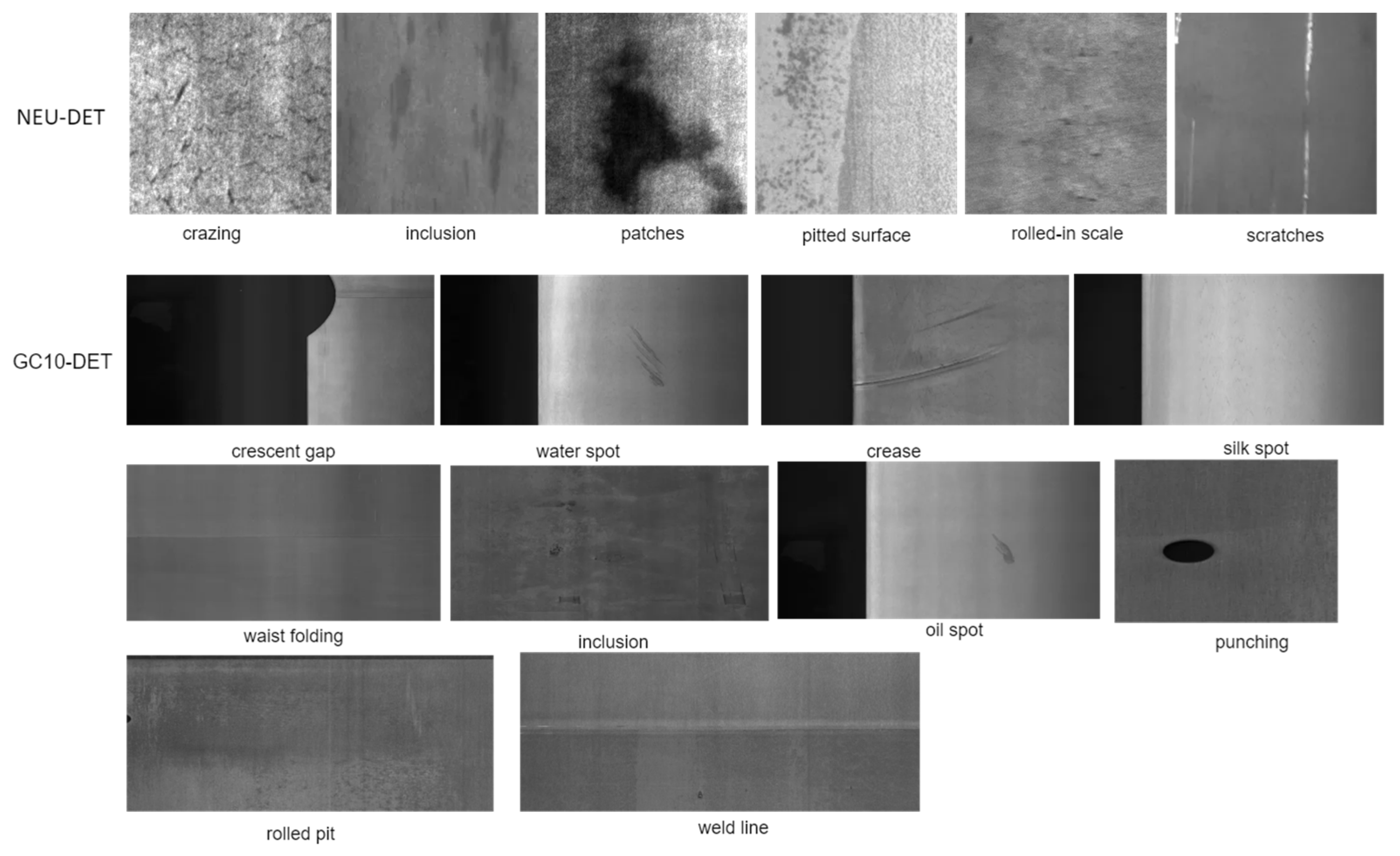
- NEU-DET is a publicly available dataset created by Northeastern University. The dataset consists of 1800 grayscale images and is divided into six different types of typical surface defects. Each type of defect contains 300 samples. These six types of defects are rolled-in scale, patches, crazing, pitted surface, inclusion, and scratches. The above six defects are all common and representative. We will describe in detail the style and reasons for each type of defect below.
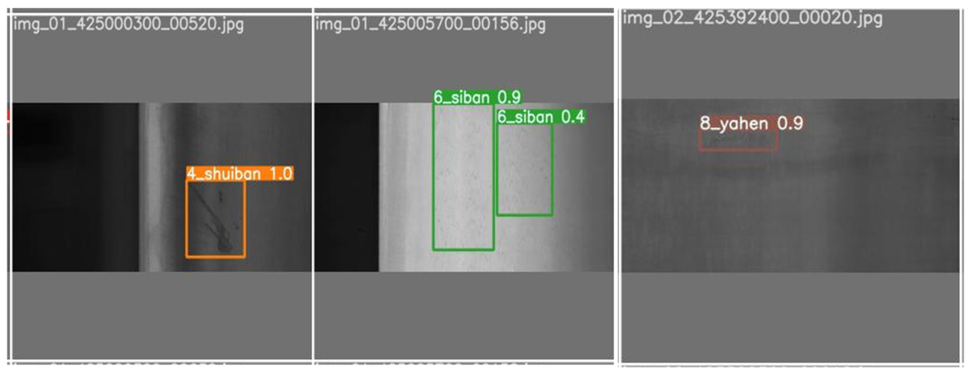
- GC10-DET is a benchmark dataset collected from real industrial scenarios provided by Lv [17]. The dataset including punching (Pu), weld line (Wl), crescent gap (Cg), water spot (Ws), oil spot (Os), silk spot (Ss), inclusion (In), rolled pit (Rp), crease (Cr), and waist folding (Wf) [18]. Compared to NEU-DET, it features 10 different types of defects, with varying numbers of images for each defect. In Figure 6, we can observe significant differences in the quantity of each type of defect.
- NEU-DET contains six types of defects, which is four fewer than GC10-DET. Additionally, NEU-DET includes 1800 grayscale images, whereas GC10-DET contains 2257 grayscale images.
- The GC10-DET dataset exhibits class imbalance, with significant differences in the quantity of each type.
- (2)
- Experimental parameters and environment
- (3)
- Evaluation indicators
4.2. Comparative Experiment
4.3. Ablation Experiments
5. Conclusions
Author Contributions
Funding
Data Availability Statement
Conflicts of Interest
References
- Arya, C.; Tripathi, A.; Singh, P.; Diwakar, M.; Sharma, K.; Pandey, H. Object detection using deep learning: A review. J. Phys. Conf. Series 2021, 1854, 012012. [Google Scholar]
- Patwal, A.; Diwakar, M.; Tripathi, V.; Singh, P. An investigation of videos for abnormal behavior detection. Procedia Comput. Sci. 2023, 218, 2264–2272. [Google Scholar] [CrossRef]
- Roka, S.; Diwakar, M.; Singh, P.; Singh, P. Anomaly behavior detection analysis in video surveillance: A critical review. J. Electron. Imaging 2023, 32, 042106. [Google Scholar] [CrossRef]
- Gangadharan, S.M.P.; Arya, C.; Aluvala, S.; Singh, J.; Singh, P.; Murugesan, A. Advancing Bug Detection in Solidity Smart Contracts with the Proficiency of Deep Learning. In Proceedings of the 2023 3rd International Conference on Innovative Sustainable Computational Technologies (CISCT), Dehradun, India, 8–9 September 2023; IEEE: New York, NY, USA; pp. 1–5. [Google Scholar]
- Li, J.; Su, Z.; Geng, J.; Yin, Y. Real-time detection of steel strip surface defects based on improved YOLO detection network. IFAC Pap. OnLine 2018, 51, 76–81. [Google Scholar] [CrossRef]
- Cheng, J.Y.; Duan, X.H.; Zhu, W. Research on metal surface defect detection by improved YOLOv3. Comput. Eng. Appl. 2021, 57, 252–258. [Google Scholar]
- Wang, Y.; Wang, H.; Xin, Z. Efficient detection model of steel strip surface defects based on YOLO-V7. IEEE Access 2022, 10, 133936–133944. [Google Scholar] [CrossRef]
- Han, D.; Yun, S.; Heo, B.; Yoo, Y. Rethinking Channel Dimensions for Efficient Model Design. arXiv 2020, arXiv:2007.00992v3. [Google Scholar] [CrossRef]
- Li, H.; Li, J.; Wei, H.; Liu, Z.; Zhan, Z.; Ren, Q. Slim-neck by GSConv: A better design paradigm of detector architectures for autonomous vehicles. arXiv 2022, arXiv:2206.02424. [Google Scholar]
- Wang, C.Y.; Bochkovskiy, A.; Liao, H.Y.M. YOLOv7: Trainable bag-of-freebies sets new state-of-the-art for realtime object detectors. arXiv 2022, arXiv:2207.02696. [Google Scholar]
- Li, H.; Kadav, A.; Durdanovic, I.; Samet, H.; Graf, H.P. Pruning filters for efficient convnets. In Proceedings of the 5th International Conference on Learning Representations, ICLR 2017, Toulon, France, 24–26 April 2017. [Google Scholar]
- Lee, J.; Park, S.; Mo, S.; Ahn, S.; Shin, J. Layer-adaptive Sparsity for the Magnitude-based Pruning. In Proceedings of the International Conference on Learning Representations, Vienna, Austria, 4 May 2021. [Google Scholar]
- Fang, G.; Ma, X.; Song, M.; Mi, M.B.; Wang, X. Depgraph: Towards any structural pruning. In Proceedings of the IEEE/CVF Conference on Computer Vision and Pattern Recognition, Vancouver, BC, Canada, 17–24 June 2023; pp. 16091–16101. [Google Scholar]
- Liu, Z.; Li, J.; Shen, Z.; Huang, G.; Yan, S.; Zhang, C. Learning efficient convolutional networks through network slimming. In Proceedings of the IEEE International Conference on Computer Vision, Venice, Italy, 22–29 October 2017; pp. 2736–2744. [Google Scholar]
- Dai, X.; Chen, Y.; Xiao, B.; Chen, D.; Liu, M.; Yuan, L.; Zhang, L. Dynamic Head: Unifying Object Detection Heads with Attentions. arXiv 2021, arXiv:2106.08322. [Google Scholar] [CrossRef]
- Ge, Z.; Liu, S.; Wang, F.; Li, Z.; Sun, J. YOLOX: Exceeding YOLO Series in 2021. arXiv 2021, arXiv:2107.08430. [Google Scholar] [CrossRef]
- Lv, X.; Duan, F.; Jiang, J.-J.; Fu, X.; Gan, L. Deep Metallic Surface Defect Detection: The New Benchmark and Detection Network. Sensors 2020, 20, 1562. [Google Scholar] [CrossRef] [PubMed]
- Xiang, X.; Wang, Z.; Zhang, J.; Xia, Y.; Chen, P.; Wang, B. AGCA: An adaptive graph channel attention module for steel surface defect detection. IEEE Trans. Instrum. Meas. 2023, 72, 1–12. [Google Scholar] [CrossRef]


| bs | Epoch | Ir | Momentum | Weight_Decay | Input_Size |
|---|---|---|---|---|---|
| 32 | 300 | 0.01 | 0.937 | 0.0005 | 640 |
| Method | P% | R% | mAP% | Params/106 | FLOPs/109 |
|---|---|---|---|---|---|
| SSD | 66.4 | 71.2 | 71.4 | 22.4 | 77.5 |
| Faster-RCNN | 73.1 | 69.2 | 77.3 | 107 | 90.9 |
| YOLOv5s | 65.6 | 70.6 | 70.7 | 7.0 | 15.8 |
| YOLOv7-tiny | 72.8 | 67.1 | 76.1 | 6.0 | 13.2 |
| ours | 67.0 | 77.9 | 79.8 | 3.5 | 9.95 |
| Method | P% | R% | mAP% | Params/106 | FLOPs/109 |
|---|---|---|---|---|---|
| SSD | 62.1 | 64.5 | 65.1 | 22.4 | 77.5 |
| Faster-RCNN | 73.2 | 69.8 | 74.1 | 107 | 90.9 |
| YOLOv5s | 74.6 | 67.1 | 73.1 | 7.0 | 15.8 |
| YOLOv7-tiny | 81.1 | 66.5 | 72.9 | 6.0 | 13.1 |
| ours | 80.1 | 72.7 | 76.4 | 4.21 | 9.9 |
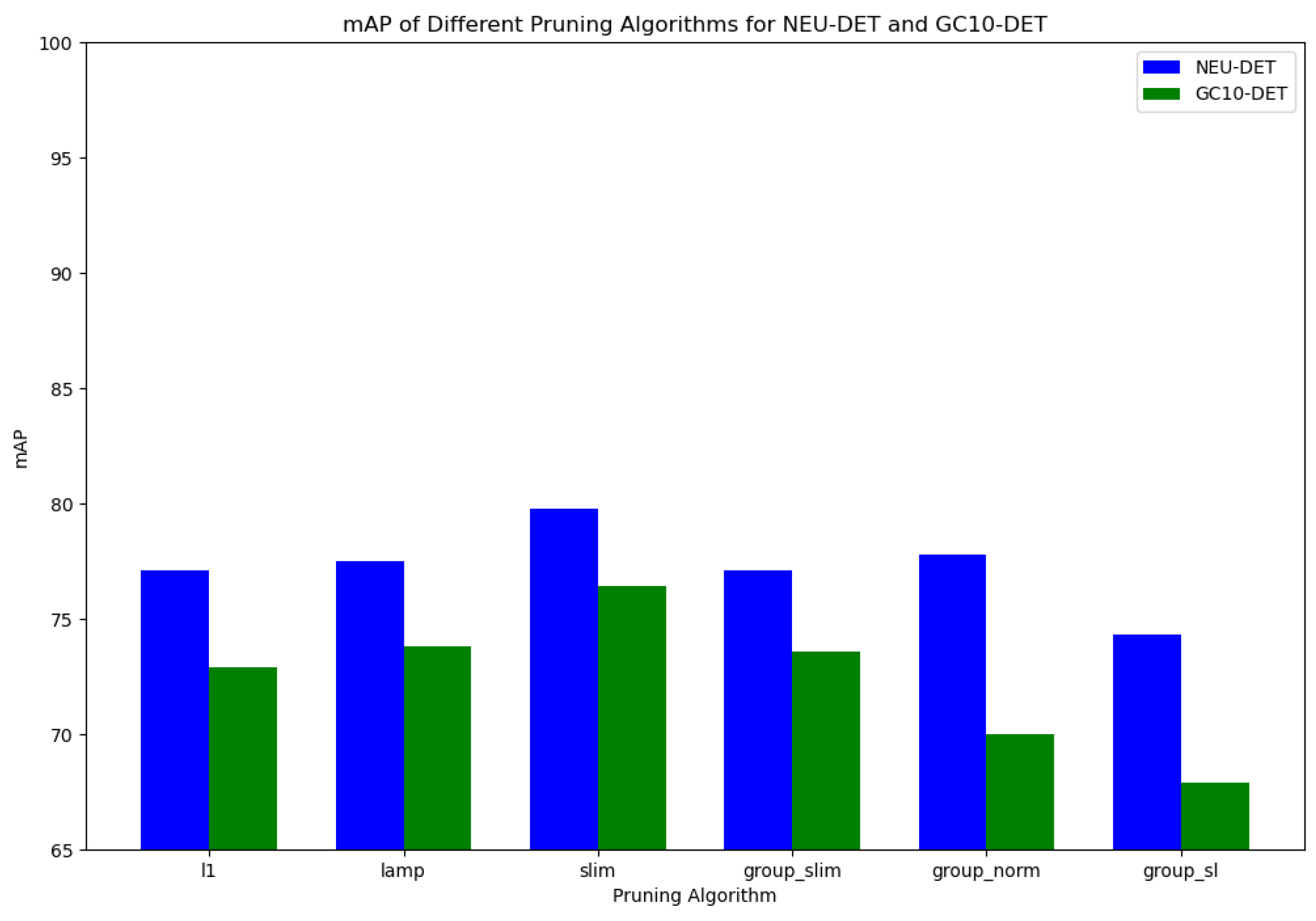
| YOLO-RDP | L1 | Lamp | Slim | Group_Slim | Group_Norm | Group_Sl | mAP% |
|---|---|---|---|---|---|---|---|
| √ | 79.2 | ||||||
| √ | √ | 77.1 | |||||
| √ | √ | 77.5 | |||||
| √ | √ | 79.8 | |||||
| √ | √ | 77.1 | |||||
| √ | √ | 77.8 | |||||
| √ | √ | 74.3 |
| YOLO-RDP | L1 | Lamp | Slim | Group_Slim | Group_Norm | Group_Sl | mAP% |
|---|---|---|---|---|---|---|---|
| √ | 74.0 | ||||||
| √ | √ | 72.9 | |||||
| √ | √ | 73.8 | |||||
| √ | √ | 76.4 | |||||
| √ | √ | 73.6 | |||||
| √ | √ | 70.0 | |||||
| √ | √ | 67.9 |
| YOLOv7-Tiny (Base) | ReXNet | GSConv + VOV-GSCSP | DdyHead | Slim Pruning | P% | R% | mAP% | Params /106 | FLOPs /109 |
|---|---|---|---|---|---|---|---|---|---|
| √ | 72.8 | 67.1 | 76.1 | 6.03 | 13.2 | ||||
| √ | √ | 66.9 | 70.5 | 70.1 | 6.65 | 12.1 | |||
| √ | √ | √ | 64.7 | 72.5 | 71.2 | 4.94 | 8.6 | ||
| √ | √ | √ | √ | 86.2 | 70.0 | 79.2 | 6.87 | 14.9 | |
| √ | √ | √ | √ | √ | 67.0 | 77.9 | 79.8 | 3.51 | 9.95 |
| YOLOv7-Tiny (Base) | ReXNet | GSConv + VOV-GSCSP | DdyHead | Slim Pruning | P% | R% | mAP% | Params/106 | FLOPs/109 |
|---|---|---|---|---|---|---|---|---|---|
| √ | 81.1 | 66.5 | 72.9 | 6.03 | 13.1 | ||||
| √ | √ | 77.5 | 67.2 | 72.4 | 6.66 | 12.1 | |||
| √ | √ | √ | 76.9 | 69.2 | 71.0 | 4.95 | 8.6 | ||
| √ | √ | √ | √ | 61.2 | 78.9 | 74.0 | 6.87 | 14.9 | |
| √ | √ | √ | √ | √ | 80.1 | 72.7 | 76.4 | 4.21 | 9.9 |
Disclaimer/Publisher’s Note: The statements, opinions and data contained in all publications are solely those of the individual author(s) and contributor(s) and not of MDPI and/or the editor(s). MDPI and/or the editor(s) disclaim responsibility for any injury to people or property resulting from any ideas, methods, instructions or products referred to in the content. |
© 2024 by the authors. Licensee MDPI, Basel, Switzerland. This article is an open access article distributed under the terms and conditions of the Creative Commons Attribution (CC BY) license (https://creativecommons.org/licenses/by/4.0/).
Share and Cite
Zhang, G.; Liu, S.; Nie, S.; Yun, L. YOLO-RDP: Lightweight Steel Defect Detection through Improved YOLOv7-Tiny and Model Pruning. Symmetry 2024, 16, 458. https://doi.org/10.3390/sym16040458
Zhang G, Liu S, Nie S, Yun L. YOLO-RDP: Lightweight Steel Defect Detection through Improved YOLOv7-Tiny and Model Pruning. Symmetry. 2024; 16(4):458. https://doi.org/10.3390/sym16040458
Chicago/Turabian StyleZhang, Guiheng, Shuxian Liu, Shuaiqi Nie, and Libo Yun. 2024. "YOLO-RDP: Lightweight Steel Defect Detection through Improved YOLOv7-Tiny and Model Pruning" Symmetry 16, no. 4: 458. https://doi.org/10.3390/sym16040458