
Improvement of Smart Grid Stability Based on Artificial Intelligence with Fusion Methods
by
 , , , and
Alaa Alaerjan
1,*,†,
Randa Jabeur
1,†,
Haithem Ben Chikha
2,†,
Mohamed Karray
3,† and
Mohamed Ksantini
4,† 1
Department of Computer Science, College of Computer and Information Sciences, Jouf University, Sakaka 72341, Saudi Arabia
2
Department of Computer Engineering and Networks, College of Computer and Information Sciences, Jouf University, Sakaka 72341, Saudi Arabia
3
ESME, ESME Research Laboratory, 94200 Ivry sur Seine, France
4
Control and Energies Management Laboratory (CEM-Lab), National Engineering School of Sfax, University of Sfax, Sfax 3038, Tunisia
*
Author to whom correspondence should be addressed.
†
These authors contributed equally to this work.
Symmetry 2024, 16(4), 459; https://doi.org/10.3390/sym16040459
Submission received: 25 February 2024
/
Revised: 29 March 2024
/
Accepted: 2 April 2024
/
Published: 10 April 2024
(This article belongs to the Section Computer)
Abstract
:It is crucial to evaluate and anticipate stability under various conditions, as the ability to stabilize a smart grid (SG) is one of its key features for assessing the effectiveness of its design. Intelligent approaches to stability forecasting are necessary to mitigate inadvertent instability in SG design. This is particularly crucial with the expansion of residential and commercial infrastructures, along with the growing integration of renewable energies into these grids. Predicting the stability of SGs is currently a major challenge. The concept of an SG encompasses a broad range of emerging technologies in which artificial intelligence (AI) plays a crucial role and is increasingly being utilized in light of the limitations of conventional methods. It empowers informed decision-making and adaptable responses to fluctuations in customer energy needs, unexpected power outages, rapid changes in renewable energy generation, or any unforeseen crises within an SG system. In this paper, we propose a symmetric approach to enhance SG stability by integrating various machine learning (ML) and deep learning (DL) algorithms, where symmetry is observed in the balanced application of these diverse computational techniques to predict and ensure the grid’s stability. These algorithms utilized a dataset containing the simulation results of the SG stability. The learning phase of these algorithms is based on imprecise and unreliable data. To overcome this limitation, the fusion of classifiers can be a powerful approach to modeling inaccurate and uncertain data, providing more robust and reliable predictions than individual classifiers. Voting and Dempster–Shafer (DS) methods, two commonly used techniques in ensemble learning, were employed and compared. The results show that the use of the fusion of distinct classifiers with voting theory achieves an accuracy of 99.8% and outperforms several other methods including the DS method.
1. Introduction
Smart grid (SG) technology is a modern electrical network that provides increased reliability, efficiency, and sustainability, along with bidirectional communication to enhance security and stability, and reduce operating costs [1,2]. Traditional grids achieve stability and balance between electricity supply and demand through demand-focused electricity production. The significant growth of the global population and economy, along with rapid urbanization, is likely to increase energy consumption demand in the coming years. Electricity, being a significant energy source, can be generated from various sources, such as water, wind, solar cells, fossil fuels, and thermal and nuclear power plants. Additionally, with progress and extensive population growth, the electricity demand continues to rise, automatically impacting the need for increased electricity production. Production, transmission, and distribution of electricity are the most critical aspects of electricity management. The electrical grid is known as an interconnected network that links consumers to electricity producers and transfers energy from producers to consumers [3]. Users play a crucial role in maintaining network stability by constantly regulating their energy needs based on the information provided by the stations. The concept of SGs is based on new information and communication technologies (ICTs). They facilitate communication in both directions between network operators, producers, and consumers. The SGs combine a variety of techniques from IT, automation, the Internet, telecommunications, and control in order to respond digitally and instantaneously to any change on the electrical network. Numerous benefits are expected to arise from the deployment of SGs. SGs must be able to perform the following:
- —
- Optimize the integration of decentralized production from renewable sources;
- —
- Manage diverse sources of production, storage, and consumption;
- —
- Increase the energy efficiency of the network;
- —
- Reduce problems caused by production variability;
- —
- Avoid the construction and reinforcement of costly power lines;
- —
- Minimize line losses;
- —
- Enhance the management of supply and demand;
- —
- Reduce consumption peaks by adjusting a portion of consumption to production.
The increase in the load on an electrical grid creates opportunities for generating additional overhead costs, leading to issues with electricity quality. These grids lack an adequate prediction system to forecast intermittent power outages, their causes, response times, storage needs, and resource utilization. Therefore, the abundance of unnecessary and irrelevant data generated during this process poses a significant problem [4]. To address this issue, the performance of SGs can be enhanced using artificial intelligence (AI) techniques by integrating various machine learning (ML) and deep learning (DL) classifiers [5,6,7,8,9]. These algorithms leverage the knowledge derived from collected data to refine the understanding of the system, optimize demand forecasts, and anticipate potential fluctuations. By dynamically adjusting network parameters in real time, SGs can proactively respond to changes, ensuring efficient energy management and improved resilience to disruptions in the electrical grid. The AI techniques not only optimize the overall network performance but also minimize operational costs while ensuring a reliable and stable energy distribution. Thus, SGs assert themselves as intelligent, adaptive, and responsive systems, making a significant contribution to the transition towards a more sustainable and efficient electrical grid. Recently, AI has served as a significant technological driver in SGs. The application of AI techniques to SGs is becoming increasingly important for modeling, optimization, and controlling. ML and DL enable intelligent decision-making and response to sudden changes in customer energy demand, unexpected disruptions in electricity supply, sudden variations in renewable energy production, or any other catastrophic events in an SG. This research paper aims to predict SG stability. For this purpose, we propose to study several ML classifiers, such as K-nearest neighbor (KNN), support vector machine (SVM), logistic regression (LR), random forest (RF), gradient boosting machine (GBM), extreme gradient boosting (XGB), and decision tree (DT). We also considered DL classifiers like recurrent neural network models (RNNs), convolutional neural networks (CNNs), long short-term memory (LSTM), and gated recurrent unit (GRU). All these models will be trained using a selected dataset containing the SG stability simulation results. In this work, we carry out a comparative analysis between the different ML and DL models based on the following evaluation metrics: accuracy, sensitivity, precision, the F1 score, the confusion matrix, and the area under the curve (AUC-ROC). This comparative study leads us to identify the classification algorithm that achieves the highest accuracy, enabling us to make better decisions regarding the prediction of SG stability. Given the inherent uncertainty in the data used for stability prediction, we employ fusion methods as introduced in [10,11] to mitigate its impact. In this case, the symmetry is further exemplified in the utilization of ensemble learning methods, such as Dempster–Shafer (DS) and voting techniques, which harmonize predictions from multiple classifiers to address the data uncertainty, showcasing a balanced and cohesive strategy toward improving SG reliability. The use of fusion methods in this research area presents an opportunity, since the studied data are uncertain, which lends more credibility to the stability prediction results.
In summary, it is crucial to emphasize that the core objective of this study is to utilize ML and DL classifiers to predict the stability of SGs. Based on the dataset, the process unfolded in three consecutive phases.
- —
- Initially, we compute the error rate for each classifier (ML and DL) to determine the optimal accuracy. It should be noted that, for this initial phase, the use of fusion methods is not included.
- —
- Subsequently, based on the last results, we combine the outputs from the most successful classifiers and calculate the fusion error rate using DS and voting methods.
- —
- Finally, we conduct a comparative analysis of the obtained results to identify the best fusion method having the highest precision.
The remainder of this paper is organized as follows: In Section 2, we present the related works. In Section 3, we expose our proposed methodology, and describe the ML and DL algorithms with the classification metrics, the belief functions theory and the voting method. Section 4 presents the experimental results and discussion. Section 5 presents the conclusion with some suggestions for further research.
2. Related Work
Conventional methods often face challenges due to the complexity and scope of the involved data, resulting in extended computation times and occasionally diminished accuracy. However, these obstacles can be effectively overcome by leveraging advanced techniques in AI and ML [12]. By harnessing these technologies, providers can gain a better understanding of consumer behaviors, enabling more precise analysis of their energy needs. This facilitates the production of accurate billing statements tailored to each user’s specific requirements. Incorporating AI and ML into SG also provides consumers with comprehensive access to their energy usage and pricing information, empowering them to proactively respond to demands for energy consumption reduction during peak periods. As a result, the operational efficiency of SGs is improved, leading to more effective management of electricity supply and demand. By integrating ICTs into SGs, consumers and producers are empowered to actively participate in ensuring the proper operation of the SG. This enables them to play an active role in monitoring and optimizing energy consumption and production, contributing to the overall functionality and efficiency of the SG system. In their work, Shi et al. [13] provided a clear overview of recent advances in using AI to analyze and control the stability of SGs. They extensively examined the definitions, historical context, and advanced methodologies of AI. Furthermore, the authors conducted a thorough exploration of various applications of AI in different aspects of SGs, such as security assessment, fault diagnosis, and stability control. Their research serves as a valuable resource for understanding how AI can enhance the stability and control of SGs. While the application of AI methodologies in SGs has demonstrated remarkable results, challenges persist, particularly concerning the extensive data, imbalanced learning, and interpretability of AI models. To address these challenges, the authors propose potential solutions, thereby promoting the continued adoption of AI for the control and analysis of SG stability.
Developing probabilistic load forecasting (PLF) is a fundamental requirement for the construction of energy-efficient and reliable SGs. PLF enables accurate prediction of future electricity demand, considering various factors and incorporating probabilities. This forecasting technique empowers grid operators to make informed decisions regarding resource allocation, load balancing, and energy management, leading to optimized planning and operation strategies. By embracing PLF, SGs can effectively integrate renewable energy sources, enhance grid stability, and ensure a balanced supply–demand interaction. Yang et al. [14] have introduced Bayesian DL as a technique to tackle the challenging task of PLF. They have proposed an innovative multitask PLF framework utilizing Bayesian DL techniques, which effectively quantifies shared uncertainties among different customer groups while considering their unique characteristics. To enhance the model’s performance and mitigate overfitting, the authors have developed a pooling method based on clustering. This increases data diversity and volume. Experimental findings indicate that the suggested model surpassed conventional methods, highlighting its improved predictive performance in PLF. Energy load forecasting plays a crucial role in the advancement of forthcoming SG systems. However, the application of conventional statistical and ML methodologies is accompanied by challenges, such as forecasting errors and a notable risk of overfitting.
The authors of [15] introduced an innovative energy load forecasting (ELF) model, which exploits deep neural network architectures for regulating energy consumption in SGs. They extensively scrutinized and simulated two deep neural network architectures—deep feed-forward neural network (deep-FNN) and deep recurrent neural network (deep-RNN)—across diverse training set sizes to assess their efficacy. Furthermore, they evaluated the performances of these architectures by experimenting with different activation functions and diverse configurations of hidden layers. The comparison of simulation results was based on the mean absolute percentage error.
Based on their findings, they were able to assert that their suggested model exhibits superior performance in contrast to existing load forecasting models. In a separate study, Kuo and Huang [16] introduced a highly precise deep neural network algorithm tailored for short-term load forecasting (STLF). They conducted a comparative analysis between their proposed model and five commonly utilized AI algorithms, namely, RF, DT, SVM, MLP, and LSTM. The primary objective was to evaluate the effectiveness of their model in accurately forecasting load in comparison to established algorithms. Their research aimed to validate the model’s capability to achieve precise load forecasting outcomes and establish its superiority over existing algorithms. With a mean absolute percentage error (MAPE) of 9.77% and a cumulative variation of root mean square error (CVRMSE) of 11.66%, their developed model demonstrated notably high accuracy in predicting load demand, thereby highlighting its effectiveness in the realm of load forecasting.
Lu et al. [17] introduced a decision system grounded in reinforcement learning aimed at aiding in the selection of electricity pricing plans. The primary objective of this system is to reduce both electricity expenses and dissatisfaction with consumption among individual end users within an SG. To tackle this, they framed the decision-making without transition probabilities, employing an enhanced state framework. Addressing computational and prediction hurdles, they utilized a kernel approximator-integrated batch Q-learning algorithm, which enhances both the efficiency and accuracy of the decision system.
3. Proposed Methodology
This section presents our methodology for SG stability.
3.1. Smart Grid Stability
The stability of electrical grids refers to the ability of an electrical system to maintain a stable equilibrium state or return to such a state after being disrupted. It is crucial for ensuring a continuous and reliable power supply. Different types of stability include voltage stability, frequency stability, and dynamic stability. These aspects are essential for ensuring the proper functioning of electrical grids.
- —
- Frequency Stability: This concerns the network’s ability to maintain its nominal frequency (e.g., 50 Hz or 60 Hz depending on the region) after a disturbance.
- —
- Voltage Stability: This refers to the network’s ability to maintain stable voltages in all parts of the electrical system after a disturbance. Voltage variations can be caused by changes in electricity demand, equipment failures, or alterations in the network configuration.
- —
- Dynamic Stability: This refers to the network’s ability to maintain or regain a stable equilibrium state in the presence of disturbances that evolve over longer periods, often due to slow variations in load or generation. This includes managing the variability of renewable energy sources such as wind and solar.
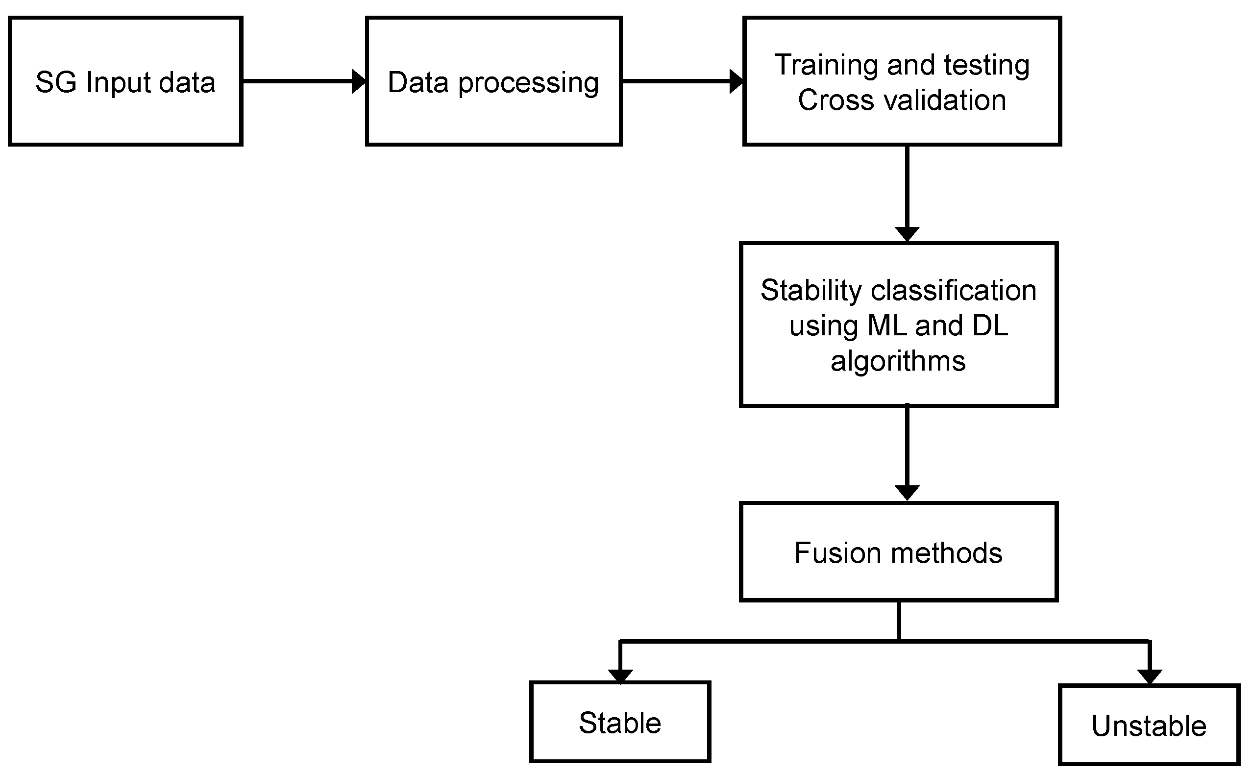
In this paper, we focus on dynamic stability. Predicting SG stability was studied based on attributes derived from the database to perform binary classification: stable or unstable. This classification was performed using ML and DL algorithms. To improve the classification results and consider the uncertain aspect of the data, fusion methods outlined by the belief function theory and the voting method were employed.
In Figure 1, we summarize all steps performed by the proposed methodology, where Algorithm 1 presents the pseudo-code.
| Algorithm 1: Pseudo-Code of the Proposed Approach |
| inputs: Smart grid stability augmented dataset outputs: Model Performance Mp
|
3.2. Dataset Processing
To be stable, electrical grids require balanced supply and demand (i.e., the electricity amount generated must match the amount consumed). In traditional power systems, balance was achieved by adjusting electricity production based on demand. This approach required a constant monitoring of electricity usage and a flexible generation system that could respond quickly to changes in demand. However, with the advent of the SG, a system of demand response was implemented. Demand response is a strategy where consumers adjust their electricity usage in response to signals from the grid. As the decentralized SG control system aims to achieve the demand response, we use a dataset originally developed by Vadim Arzamasov [18]. The decentralized SG control system model is made up of two primary components:
- —
- Simulation of energy production and consumption: This component represents the various entities that are connected to the grid, each of which could be a consumer, a producer, or both. For instance, a residential home might consume electricity, a solar farm might produce electricity, and a building with solar panels might do both. This simulation takes into account the quantity of electricity each participant produces or consumes, the timing of this production or consumption, and any constraints they might have.
- —
- Modeling of electrical energy price variation: This component of the model is concerned with how the price of electrical energy changes in response to the grid’s frequency. In a functioning power grid, the frequency must be kept within a certain range to ensure stability. If the frequency deviates too far from this range, it can indicate an imbalance between supply and demand, which can lead to instability. To manage this, the price of electricity can be adjusted.
The considered dataset, available in [19], contains 60,000 data points. This dataset was obtained through 10,000 simulations using the decentralized SG control system with the following six input values:
- —
- Damping constant (i.e., the efficiency of a control system in modulating its power output to uphold the stability of the grid frequency);
- —
- Coupling strengths (i.e., the level of interaction and mutual influence between different subsystems within the grid);
- —
- Averaging time (i.e., the period over which data are collected and averaged to smooth out short-term fluctuations and highlight longer-term cycles);
- —
- Price elasticity (i.e., the fluctuation in energy consumption relative to alterations in prices, while holding all other factors constant);
- —
- Reaction time (i.e., the duration taken by participants to respond in adjusting their consumption and/or production concerning price variations);
- —
- Mechanical power (i.e., the physical energy that is converted into electricity by mechanical generators, such as wind turbines or hydroelectric dams).
Note that the simulation was conducted using a configuration consisting of a single producer node and three consumer nodes interconnected in a star topology. The individual data points were generated by randomly selecting values for the input variables specified in the dataset description. Subsequently, the system stability was computed based on these simulations.
The study’s dataset incorporates 12 characteristics essential for analysis and prediction purposes. These predictive characteristics include:
- —
- Response time—producer of energy.
- —
- Response time—user_1.
- —
- Response time—user_2.
- —
- Response time—user_3.
- —
- Balance of forces—producer of energy.
- —
- Balance of forces—user_1.
- —
- Balance of forces—user_2.
- —
- Balance of forces—user_3.
- —
- Price elasticity coefficient (gamma)—producer of energy.
- —
- Price elasticity coefficient (gamma)—user_1.
- —
- Price elasticity coefficient (gamma)—user_2.
- —
- Price elasticity coefficient (gamma)—user_3.
The prediction outcome involves two categories:
- —
- Stable.
- —
- Unstable.
The ‘1’ label has been assigned to denote a stable grid condition, whereas the ‘0’ label represents an unstable grid condition. The dataset comprises features with different dimensions and scales combined. This could potentially impact the model’s fitting process and result in biased predictions, leading to errors in classification and inaccurate rates of precision.
In order to mitigate this issue, standardization was performed before fitting the framework. This process involved adjusting the features in the dataset to a standardized scale, i.e., mean (µ) = 0 and standard deviation () = 1.
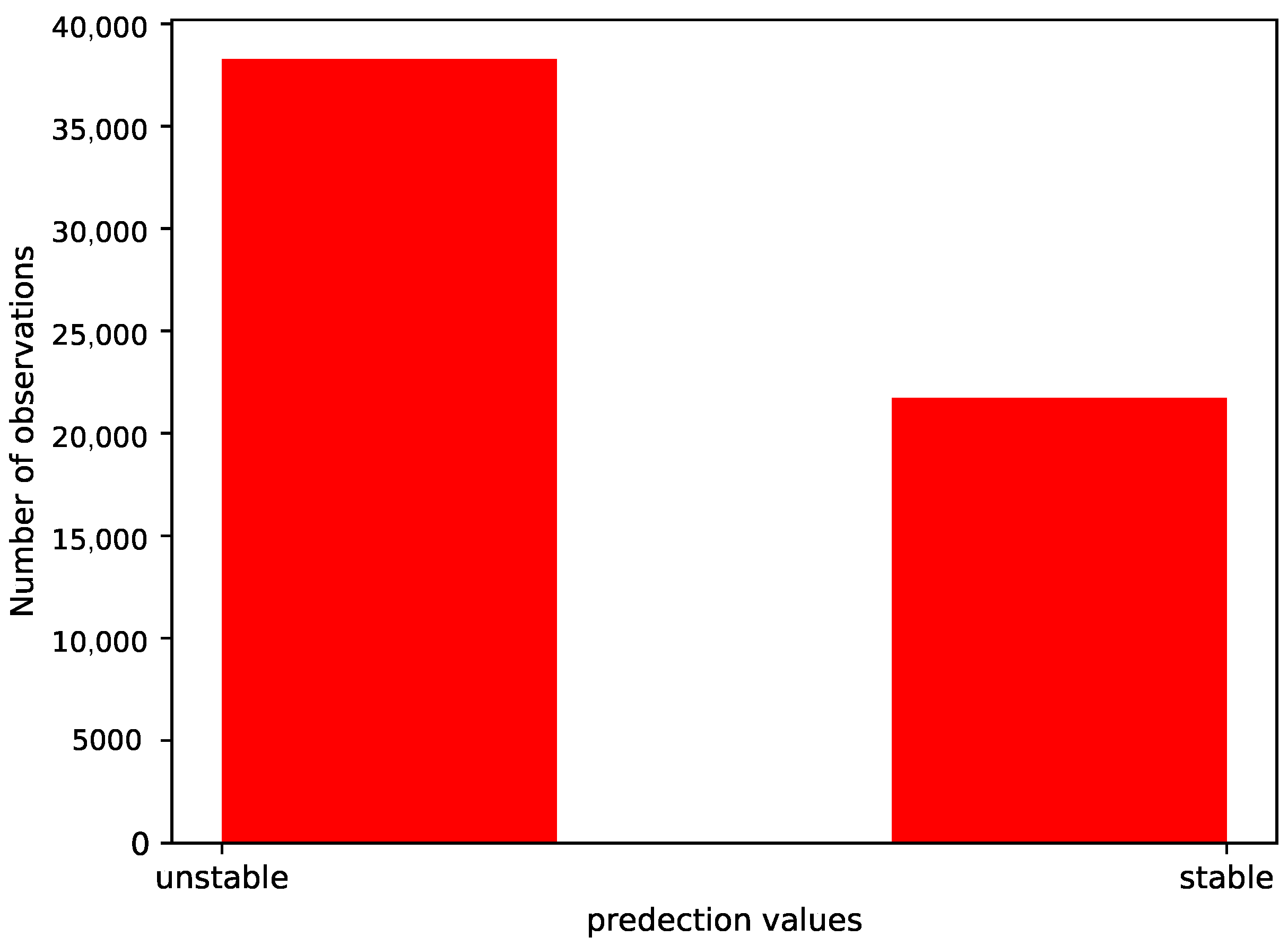
The dataset is balanced if the positive values are approximately the same as the negative values.
The dataset is imbalanced if there is a significant disparity between the positive and negative values. Figure 2 presents the distribution of the predictive states. It shows that the dataset is imbalanced.
3.3. ML Algorithms Based on Supervised Classification
Supervised classification mirrors human learning by leveraging past experiences to gain new knowledge and understanding. In this approach, machine learning algorithms are trained using a dataset containing pre-classified instances and their corresponding predicted values. From this training set, the algorithm constructs a preliminary model, enabling it to predict missing values in incomplete datasets [20]. This section will delve into popular methods commonly employed in supervised classification, briefly outlining their operating principles, strengths, challenges, and application areas. Furthermore, recent advancements in these methods will be explored. Specifically, the following ML algorithms have been used to forecast the stability of the SG.
3.3.1. Support Vector Machine
SVM represents a suite of supervised learning techniques primarily applied to binary classification tasks but extends its utility across diverse fields like bioinformatics and finance [21]. SVM delineates a boundary maximizing the separation distance between various data categories, even in scenarios where the data are not linearly separable. It accomplishes this by projecting data into a higher-dimensional attribute space and crafting optimal separation hyperplanes [22]. SVM exhibits efficacy in managing high-dimensional spaces and excels with unstructured and semi-structured data formats. The choice of kernel function significantly influences SVM’s aptitude to tackle intricate problems. Nonetheless, SVM encounters challenges when there is substantial overlap between target classes and its performance may falter if the number of characteristics per data point surpasses the count of training data samples. Under such circumstances, the selection of an optimal kernel presents a formidable task [23].
3.3.2. Logistic Regression
LR stands as a widely used statistical method specifically designed for binary classification tasks. It belongs to the family of regression analyses wherein the dependent variable, often termed as the outcome or response variable, assumes categorical values, typically denoted as 0 and 1. The principal aim of logistic regression lies in estimating the probability that a given input pertains to a particular category. This is achieved by modeling the relationship between the inputs and the probability of the outcome utilizing the logistic function, also recognized as the sigmoid function. In essence, logistic regression facilitates the estimation of the probability or risk associated with a particular outcome based on the value(s) of the independent variable(s) [24].
3.3.3. K-Nearest Neighbor
KNN is a straightforward supervised learning approach applicable to regression and classification tasks [25]. It is a non-parametric method that involves storing the training set’s observations to classify new data from the testing dataset. To forecast the category of new input, the KNN algorithm follows a simple procedure: First, it calculates the Euclidean distance between the target object for classification and all other objects within the dataset. Then, using these distance quantities, it selects the nearest neighbors. Finally, the class for the object is determined by performing a majority vote among the classes of the nearest neighbors [26]. The Euclidean distance is a prevalent distance function, computed in the following manner [27]:
where and represent the m attribute values. KNN method is employed for object classification in various fields such as text classification, human activity recognition, computer vision, handwriting recognition, and trajectory analysis [28]. The KNN algorithm boasts several advantages, including its simplicity, ease of understanding, and straightforward implementation. It is relatively quick to learn and can yield satisfactory performance. KNN also excels in defining the distribution of class data, providing useful insight into the underlying patterns. Consequently, it is regarded as one of the most powerful approach in the field of machine learning [29].
3.3.4. Decision Tree
The method presented here is employed for addressing regression and classification issues. Its purpose is to construct a training model of forecasting the class or value of the target variable by leveraging historical decision rules. The process begins with a root in the form of a tree, which then branches out, forming interconnected nodes, and culminates in leaves that are associated with specific classes to be predicted. Each node within the tree signifies a distinct rule and traversing the tree entails evaluating a sequence of these rules. To traverse the tree implies examining a sequence of rules. In essence, this method is an algorithm for rule-based classification, where the rules are acquired by partitioning the training data in a manner that maximizes the number of accurate classifications [30].
The DT algorithm is highly effective in addressing nonlinear problems. It excels at handling both numerical and categorical data simultaneously. Compared to other algorithms, it requires less data filtering. However, it consists of multiple layers, rendering it complex and, consequently, the computational complexity of the decision tree escalates when faced with a substantial quantity of class labels [31].
3.3.5. Random Forest
RF classifier is renowned for its versatility in tackling both classification and regression tasks. Initially, the algorithm commences at the root node of a tree, encompassing the entire dataset. Subsequently, it assesses the efficacy of each predictor variable in distinguishing between different nodes. Typically, this tree-based approach involves pruning the tree to an optimal size, mitigating overfitting, a process typically facilitated through cross-validation [32]. Implementing RF necessitates the configuration of two primary parameters: the number of trees (ntree) and the selection count of predictor variables chosen at random (mtry).
3.3.6. Gradient Boosting Machine
Much like RF, GBM serves as another technique employed in supervised machine learning tasks, spanning various classification and regression scenarios. GBM assembles a prediction model by amalgamating multiple weak prediction models, typically decision trees, to form an ensemble [33]. It comprises three pivotal components: (i) a loss function intended for optimization, (ii) a weak learner entrusted with making predictions, and (iii) an additive model that integrates weak learners to enhance loss function optimization [34]. GBM entails three primary tuning parameters: the maximum number of trees (ntree), the maximum depth of interactions among independent variables (tree depth), and the learning rate, alternatively referred to as shrinkage [35].
3.3.7. Extreme Gradient Boosting
XGBoost has emerged as a prominent machine learning model, significantly advancing tree-boosting algorithms in recent years. This system generates a prediction model by employing gradient descent to optimize the loss function, ultimately yielding a boosting ensemble of weak classification trees [36]. Notably, XGBoost demonstrates exceptional efficiency in reducing processing time and is versatile, and applicable to both regression and classification tasks. The parameters of the XGBoost algorithm are categorized into three groups, as outlined by Chen et al. [37]: General Parameters, Task Parameters, and Booster Parameters. In the context of the work, three specific general parameters were selected to fine-tune the XGBoost algorithm during the application of the Local Sensitivity Method (LSM): colsample_bytree (the subsample ratio of columns when constructing each tree), subsample (the subsample ratio of the training instances), and n rounds (the maximum number of boosting iterations).
3.4. Implementation of DL Classifiers
DL algorithms encompass a category of ML methods rooted in artificial neural networks comprising multiple layers. These algorithms are engineered to autonomously learn and extract hierarchical data representations by employing interconnected layers of nodes, commonly referred to as neurons or units. Numerous DL algorithms have been devised and deployed to forecast the resilience of the SG.
3.4.1. Neural Network
The initial layer of the neural network is referred to as the input layer, where data are fed into the network. Conversely, the final layer is known as the output layer, responsible for providing the classification results. The input and output layers are considered the hidden layers [38]. A network becomes deeper as it incorporates more hidden layers. The network parameters are iteratively adjusted through a process known as backpropagation.
3.4.2. Convolutional Neural Networks
CNNs consist of multiple layers and are mainly employed for tasks such as image processing, time series prediction, and identifying and categorizing anomalies in objects. These networks incorporate extra layers known as “filtering” layers, which enable the learning of filter coefficients or convolutional filters, alongside weights and biases assigned to individual neurons [39]. The operational mode of a CNN involves multiple layers that process and extract information [39]. These layers include:
- —
- Convolution layer: This comprises multiple filters tasked with executing the convolution operation on the input data.
- —
- Rectified linear unit (ReLU): This layer conducts operations on the data, producing a rectified feature map as its output.
- —
- Pooling layer: The rectified feature map is subsequently forwarded through a pooling layer, which conducts subsampling and diminishes the dimensions of the feature map.
- —
- Connected layer: This layer is constructed using the flattened array from the pooling layer as its input, facilitating image classification and identification.
3.4.3. Recurrent Neural Networks
RNNs have gained significant popularity in the field of DL [40,41,42]. Although they were developed in the 1980s, their widespread adoption has occurred only in recent years due to advancements in computing power and the availability of massive amounts of data. RNNs are unique neural networks that enable information propagation in both forward and backward directions, mimicking the functionality of the nervous system. These networks possess recurrent connections, allowing them to retain and utilize data in their memory. RNNs, or Recurrent Neural Networks, are designed to process sequential data effectively by utilizing previous outputs as additional inputs. This unique characteristic enables RNNs to achieve high prediction accuracy. In the operating mode of an RNN layer, the inputs are sequentially traversed, moving from to and beyond. At each time step t, the last cell of the RNN combines the current input with the prediction from the previous step to compute the output ht. The resulting vector ht serves as the final output of the RNN layer. This process establishes the recurrence relation defined by the RNN layer.
3.4.4. Long Short-Term Memory
The activation function used in RNNs, specifically the tanh function, often encounters a large number of values nearing zero frequently during derivative computations. Additionally, classical RNNs have a tendency to remember only recent information before forgetting it. To address these limitations, LSTM employs the sigmoid function and possesses an internal memory that is dynamically and constantly changing based on the input data. This enables LSTMs to overcome the mentioned issues [43,44]. LSTM networks extend the capabilities of RNNs by introducing an extended memory mechanism. They allow “weights” to the data, enabling RNNs to process new inputs and either forget them or give them the significance to influence the output. In the context of LSTMs, the hidden units are referred to as the following [42]:
- —
- Forget gates: These gates identify and retain pertinent information from the past.
- —
- Input gates: These gates choose and incorporate information from the present input that is deemed important for long-term memory storage.
- —
- Output gates: These gates select crucial information from the new cell state to create the following hidden state and output.
Due to their complex architecture, the learning phase of LSTMs necessitates a greater amount of time in comparison to traditional neural networks or RNNs. However, LSTMs achieve significantly improved performance. The LSTM network also employs a recurrent expression but introduces an additional variable known as the cell state c to defer the recurrence.
In the LSTM architecture, data are conveyed from one cell to the next via two channels: h and c. At time t, the updates to these two channels are determined by the interaction between their preceding values and and the current element of the input sequence . In [44], there is a comprehensive understanding of the LSTM architecture including the specific equations involved.
3.4.5. Gated Recurrent Unit
The GRU represents the latest advancement in RNN models and offers notable enhancements compared to both RNNs and LSTMs. Unlike the RNN, the GRU incorporates two key gates known as the update gate and reset gate [44,45,46,47], within each GRU unit, instead of the three gates found in an LSTM cell. The update gate in a GRU plays a crucial role in determining the extent to which past data should be retained and transmitted to the following conditions. To elaborate on the process, the reset gate of the GRU initiates by storing significant information from the previous time step in a separate memory space. Subsequently, it performs element-wise multiplications between the input vector and the hidden state, taking into account their respective weights. This multiplication is further combined with the product of the reset gate and the previous hidden state. In the last, the resulting sum is passed through an activation function, as described in [44].
3.5. Fusion Methods
ML and DL algorithms play a crucial role in prediction and classification tasks, aiming to achieve more accurate decisions. In decision support systems, where vast amounts of data are involved, such as medical imaging, satellite or radar imagery analysis, climate prediction, and signal and image processing, the scale of information is immense. Moreover, these data are frequently characterized by imprecision, uncertainty, vagueness, and incompleteness, posing additional challenges to the analysis and interpretation process. The presence of such factors introduces challenges in representing knowledge effectively. This can occur due to insufficient numerical information or the utilization of natural language terms to describe certain attributes. Uncertainty arises concerning the reliability and accuracy of the data itself. The source providing the data can be unreliable, prone to errors, or deliberately delivering false data. Consequently, the data obtained are partial and prone to inaccuracy. In this framework, uncertainty in SG data refers to the lack of precise or complete knowledge about certain aspects of the network’s operation, performance, or environmental conditions. This uncertainty can arise from various sources and may impact decision-making processes and the overall reliability of the SG. For example, in renewable energy generation, the output of renewable energy sources like solar and wind power is inherently uncertain due to weather conditions. Also, in an SG, data are collected from various sensors and devices. Communication errors, sensor inaccuracies, or device malfunctions can introduce uncertainty into the data, affecting the accuracy of monitoring and control systems. Addressing and managing uncertainty in SG data is crucial for making informed decisions, improving grid resilience, and ensuring the efficient and secure operation of the electrical network. To address the challenges posed by imprecision and uncertainty, it becomes crucial to employ formalisms that can effectively model these imperfections. Furthermore, in order to maximize the utilization of available information, these formalisms need to incorporate fusion mechanisms, such as combination or aggregation techniques [48]. This fusion phase enables the generation of synthesized information that can aid in decision-making processes. Among these formalisms, we will describe the theory of belief functions and the voting method.
3.5.1. Belief Functions
Belief functions stem from the pioneering work of Arthur Dempster in generalizing Bayesian formalism [49]. Glenn Shafer played a considerable role in formalizing the credal aspect of the theory, leading to the development of the DS method, also known as the theory of evidence. This theory, rooted in probabilistic mathematics, establishes an official setting for making deductions amid uncertainty, providing a means to model knowledge effectively. Through the use of belief functions, which serve as tools for assessing subjective probabilities, we can assess the level of truthfulness in a given assertion. By incorporating measures of evidence, coefficients of weakening, and the rule of combination, this framework enables the treatment of information derived from diverse sources across different fields, ultimately attaining a level of reliability. The utilization of the DS theory proves highly beneficial in the decision-making process [50]. The DS theory can be summarized through the following steps [51]: Initially, we express the available information in the form of mass functions. The mass function, denoted as m, represents the discerning frame and is defined as follows:
By incorporating the belief degree regarding the reliability of the source, we apply the mass function m to rectify the data. Consequently, we obtain a revised mass function that can be described as follows:
Ultimately, we integrate the information to arrive at the optimal decision. In this scenario, we take into account two sources, each represented by the mass functions and . The fusion of these two sources results in a new mass function, which can be represented as follows:
To ensure an informed decision-making process following the fusion step, the pignistic transformation plays a crucial role. This transformation is defined as a probability distribution, represented by the following:
The decision is made based on the pignistic transformation by selecting the element x that possesses the highest probability:
The DS fusion theory offers the advantage of enabling decision-making even in the event of classifier failures. Additionally, this theory allows classifiers, despite utilizing different learning algorithms, to approach and solve a given problem from diverse perspectives.
3.5.2. Voting Method
The voting method represents a direct and efficient fusion strategy, impartial to any single classifier. However, it is important to recognize that each classifier’s performance can fluctuate depending on the context. Therefore, evaluating its effectiveness necessitates considering the significance or precedence of individual classifiers under particular conditions. This aspect has received thorough examination within the fault classification domain [52,53]. The voting method is given by the following:
where is the classifier and is the weight associated with the classifier’s prediction. The voting method supports two voting approaches:
- —
- Hard Voting: The voting classifier estimator predicts the output by selecting the class that garners the greatest number of votes from each classifier. Hard voting is distinguished by its simplicity and ease of application. It simply involves choosing the class with the most votes, making it simple and intuitive. The effectiveness of hard voting is demonstrated when the individual classifiers in the ensemble are diverse and their errors are not significantly correlated. In such situations, merging their decisions through majority voting can lead to more robust and accurate predictions.
- —
- Soft Voting: The prediction of the output class relies on the mean probability attributed to that class. If ’hard’ is chosen, the predicted class labels are used for the majority vote, while ’soft’ relies on the argmax of the summed predicted probabilities. The ’soft’ approach is recommended for a set of well-calibrated classifiers. Soft voting can be more robust in situations where models present different levels of uncertainty. It enables the most reliable models to make a greater contribution to the final decision. Also, it can improve overall performance, particularly when it comes to combining well-calibrated models that provide accurate probability estimates.
4. Results and Discussion
4.1. Classification Measures
In a classification problem, the potential values can be outlined as follows:
- —
- True positives (TP): The count of positive instances correctly identified as positive.
- —
- True negatives (TN): The count of negative instances correctly identified as negative.
- —
- False positives (FP): The count of negative instances incorrectly identified as positive.
- —
- False negatives (FN): The count of positive instances incorrectly identified as negative.
The metrics employed to assess the classification are accuracy, precision, recall, and F1 scores:
- —
- Accuracy in classification models is determined by dividing the count of accurate predictions by the total number of predictions made during the evaluation. The accuracy is given by
- —
- Precision, often known as positive predictive value, gauges the ratio of accurately classified positive instances to the total number of instances predicted as positive by the model. The precision is given by
- —
- Recall, also known as sensitivity or true positive rate, quantifies the ratio of correctly classified positive instances to the total number of positive instances in the dataset. The recall is given by
- —
- The F1 score is a metric that integrates precision and recall into one value by computing their harmonic mean. This offers a balanced evaluation of the classification model’s effectiveness. The F1 value is given by
In our case, the number of states exhibits an imbalanced distribution, as depicted in Figure 2. To address this issue, the weighted-averaged score, which considers precision, recall, and F1 score, is employed to mitigate the impact of the weakest scores. The weighted average is computed by averaging the precision, recall, and F1 scores for each class, while taking into account the support of each class. Support denotes the real count of occurrences for each class within the test database. Among these metrics, the F1 score is considered more suitable as it represents the harmonic mean of precision and recall. By using the F1 score, a balance between precision and recall is maintained, and the score is improved only if the classifier accurately identifies more instances of a specific class.
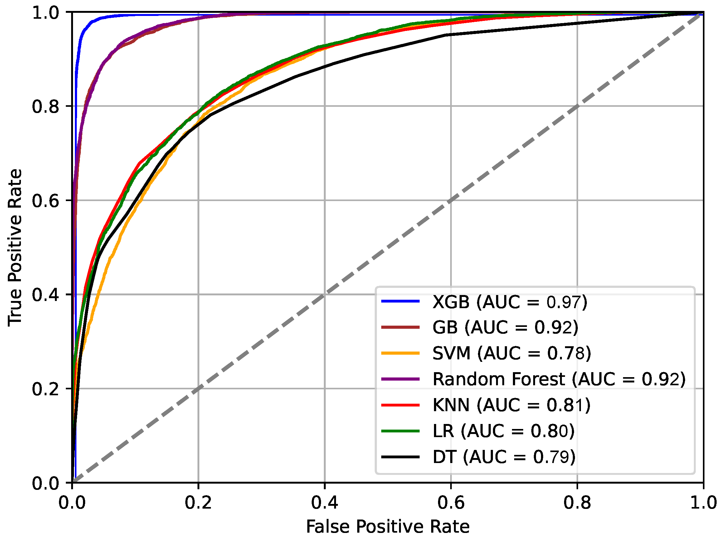
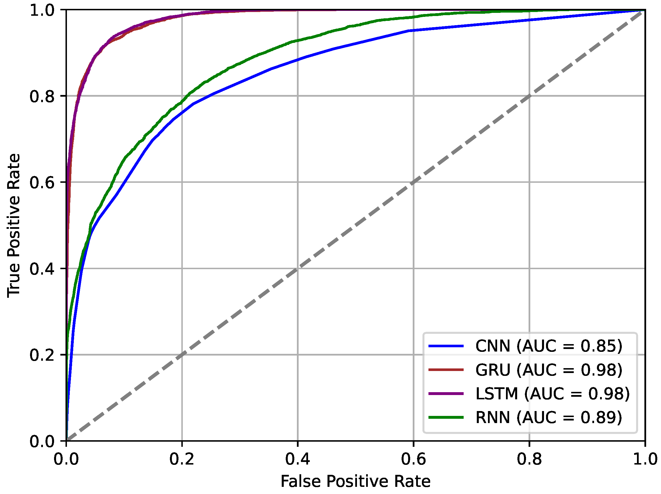
The performance of classification results can also be assessed using the AUC-ROC (Area Under the Receiver Operating Characteristic) ROC curve, a commonly employed evaluation metric for binary classification tasks. It assesses the classifier’s capability to differentiate between the two classes. The AUC represents the area under the curve, with the false positive rate plotted on the x-axis and the true positive rate plotted on the y-axis. An excellent model should have an AUC close to 1, indicating a high degree of separability between the classes. This means that the model can effectively distinguish between the positive and negative instances.
Similarly, the precision–recall (PR) curve is used for evaluating binary classification algorithms. The AUC-PR is derived by mapping precision against recall across different threshold values. Precision measures the ratio of accurately classified positive instances among all instances predicted as positive, while recall quantifies the ratio of accurately classified positive instances among all actual positive instances. Likewise, an AUC-PR score closer to 1 indicates better classifier performance, as it signifies a higher precision and recall trade-off.
Google Collaboratory is used as a framework for training and testing ML and DL algorithms. This cloud service offers approximately 12 GB of RAM and GPU support that can be expanded to 25 GB.
4.2. Results on Independent Classifiers
After calculating the measures of Equations (10)–(13), the accuracy for each ML and DL classifier is shown, respectively, in Table 1 and Table 2.
4.3. DS Fusion Results
4.3.1. ML Results
In this section, we employ DS theory combining seven ML classifiers provided with the following mass functions, , and , respectively, for the XGB, GB, SVM, RF, KNN, LR, and DT classifiers. First, we fuse all classifiers. The classification rate is then tested by combining the three best classifiers RF, XGB, and GB. Thus, two types of combination (data fusion) between classifiers are obtained according to the mass combination DS rules:
- —
- ;
- —
Using the pignistic transformation of the acquired masses enables us to accomplish a determination regarding the fusion results. Table 3 displays the results of the fusion for two various combinations of classifiers for the ML algorithms based on the DS theory. The fusion of all algorithms gave 89% accuracy. However, it achieved 82% when combining the RF, XGB, and GB classifiers.
4.3.2. DL Results
In this section, we employ DS theory combining four DL classifiers presented by the mass function s , and , respectively, for each classifier CNN, GRU, LSTM, and RNN. First, we fuse all classifiers. The classification rate is then tested by combining the two best classifiers, GRU and LSTM. Thus, two types of combination (data fusion) between classifiers are obtained according to the mass combination DS rules:
- —
- ;
- —
The pignistic transformation of the obtained masses allows us to determine the fusion results. Table 4 displays the results of the fusion of the two various combinations of classifiers for the DL algorithms based on the DS theory. The obtained accuracy, for the fusion of all classifiers, is 92%. By fusing the GRU and LSTM classifiers, the accuracy is 93%.
4.4. Voting Fusion Results
Applying the soft and hard voting approaches, the results of fusion classifiers based on ML and DL are presented in the following sections.
4.4.1. ML Results
This section presents the results of the voting fusion approach based on ML algorithms. Table 5 displays the accuracy results. As seen from these results, using soft voting, the fusion of the RF, XGB, and GB classifiers achieves 99.8%.
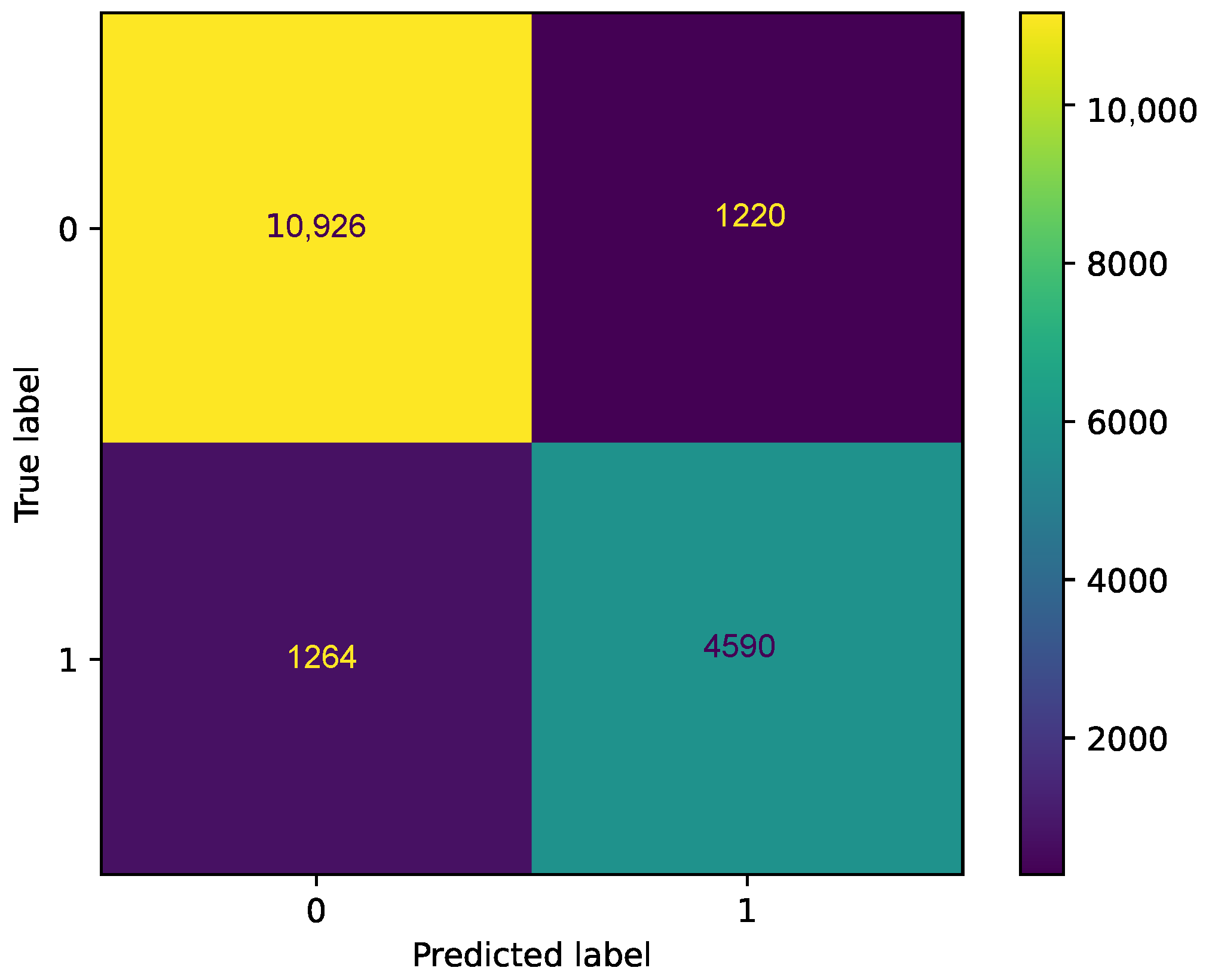
Figure 5 presents the confusion matrix for the seven ML classifiers. Here, the TP, TN, FN, and FP for the seven ML classifiers using voting theory are 10,531, 4670, 1615, and 1184, respectively. The TP and TN indicate that the predictions are accurate. The FP indicates that the model incorrectly predicts the positive class. The FN indicates that the model fails to identify and predict the positive class.
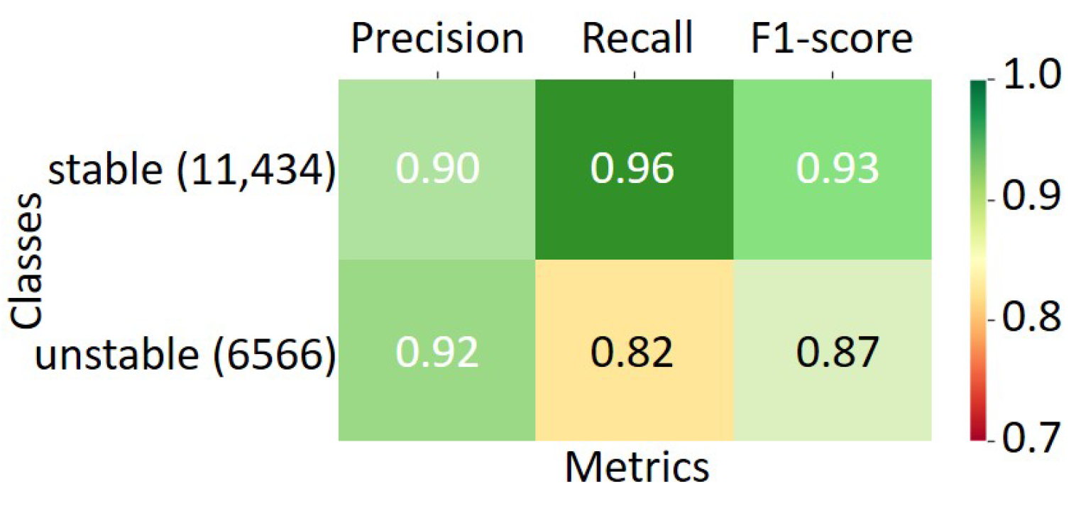
Figure 6 shows the classification for the seven ML classifiers. It effectively demonstrates the merits of the voting method in predicting the SG stability, yielding good stable classification results.
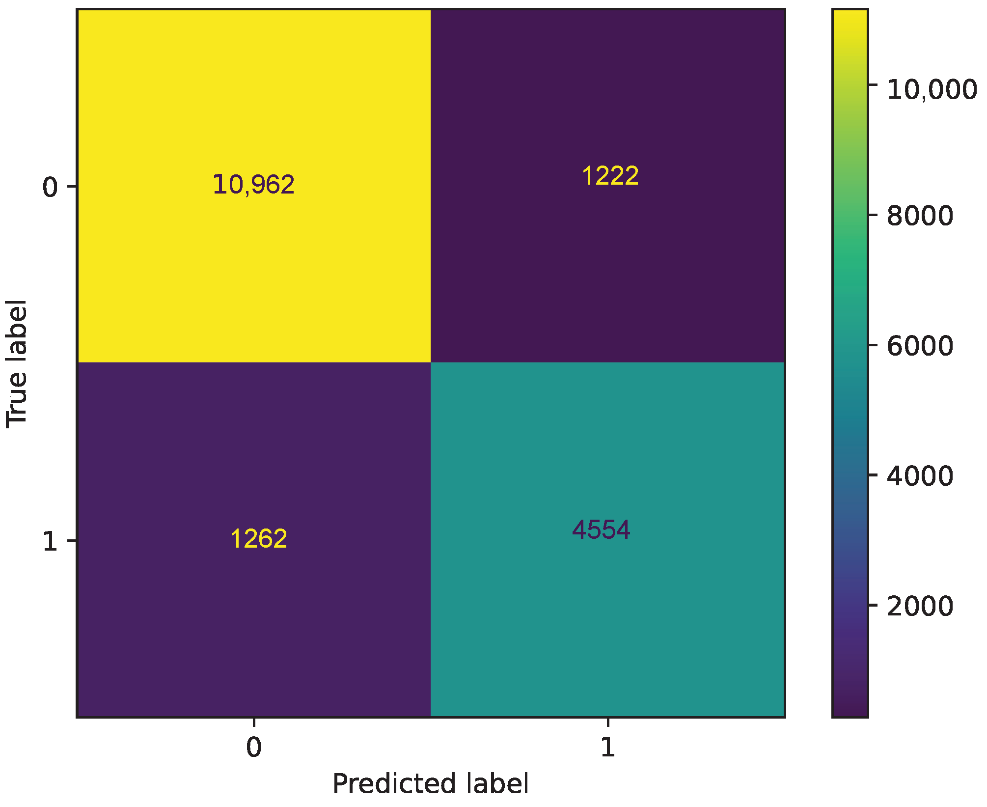
In Figure 7, we present the confusion matrix for the three best ML classifiers. Here, one can observe that the use of the three best ML classifiers offers a better prediction compared to the case where we use seven classifiers.
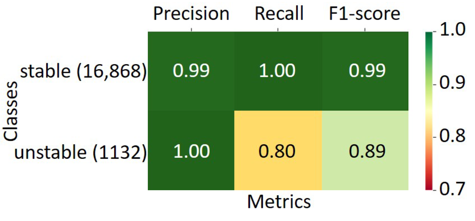
In Figure 8, we show the binary classification of predicting the SG stability using the three best ML classifiers. As seen from these results, the prediction performance in this case outperforms the one using seven ML classifiers.
4.4.2. DL Results
This section presents the results of the voting fusion approach based on DL algorithms.
Table 6 displays the accuracy results. Here, the fusion of the GRU and LSTM classifiers achieved 99% using soft voting.
The confusion matrices for all and the two best DL classifiers are depicted in Figure 9 and Figure 10, respectively. In Figure 9, one can see that the TP, TN, FN, and FP for all DL classifiers using voting theory are 9226, 5094, 1660, and 2116, respectively. Also, the FP indicates that the model incorrectly predicts the positive class and the FN indicates that the model fails to identify and predict the positive class. Compared with Figure 5, the results obtained with the ML case are better.
4.5. Comments on Results
Based on the above results we concluded some points:
- —
- The ML results based on the voting fusion approach gave the best performances (99.8%) compared with those obtained with DL algorithms (99.6%).
- —
- The fusion ML results surpassed those obtained with the fusion DL classifiers as well as with the independent classifiers.
- —
- The merits of the voting method are well proved in this work since the accuracy obtained with the voting method is better than those obtained with the DS theory.
- —
- —
- In this study, leveraging fusion techniques proves advantageous as it addresses the inherent uncertainty within the data. By integrating multiple sources of information, we effectively maximize the utility of available data, consequently enhancing both the quality and reliability of the foundational dataset.
5. Conclusions
This study proposed a prediction approach based on AI techniques to enhance the stability of the SG network. The SG dataset was trained using various ML and DL algorithms. Since the learning phase of these algorithms relied on imprecise, uncertain, and unreliable data, we employed two fusion methods known as the belief functions and the voting methods, in order to overcome these limitations. The classification accuracy, sensitivity, precision, and F1 score, the confusion matrix, and the AUC-ROC curve are used to evaluate the performance of ML and DL algorithms, without and with the fusion methods. The test results are performed and demonstrated the accuracy and feasibility of the voting fusion method while determining SG stability. Thus, the results obtained with the voting method were superior to those obtained with the belief functions method, achieving an accuracy of 99.8%.
Future work will consist of extending this research by using an SG dataset including additional energy sources to better predict the SG stability. Another important research axis is related to the improvement of the obtained accuracy by exploring advanced techniques based on DL, such as reinforcement learning and transfer learning.
Author Contributions
Conceptualization: A.A. and R.J.; methodology: M.K. (Mohamed Karray), M.K. (Mohamed Ksantini) and H.B.C.; validation: H.B.C., M.K. (Mohamed Ksantini) and M.K. (Mohamed Karray); formal analysis: R.J. and A.A.; writing—original draft preparation: H.B.C., M.K. (Mohamed Karray) and M.K. (Mohamed Ksantini); writing—review and editing: A.A. and R.J.; supervision: R.J., M.K. (Mohamed Ksantini), M.K. (Mohamed Karray), A.A. and H.B.C. All authors have read and agreed to the published version of the manuscript.
Funding
This research was funded by the Deputyship for Research & Innovation, Ministry of Education in Saudi Arabia through the project number 223202.
Data Availability Statement
Data are contained within the article.
Conflicts of Interest
The authors declare that there were no disclosed possible conflicts of interest relevant to the research.
References
- Fang, X.; Misra, S.; Xue, G.; Yang, D. Smart:Smart grid—The new and improved power grid: A survey. In Proceedings of the IEEE Commun Surveys Tutor, Washington, DC, USA, 4–6 June 2012; Volume 14, pp. 944–998. [Google Scholar]
- He, Y.; Mendis, G.J.; Wei, J. Real-time detection of false data injection attacks in smart grid: A deep learning-based intelligent mechanism. IEEE Trans Smart Grid. 2017, 8, 2505–2516. [Google Scholar] [CrossRef]
- Morello, R.; De Capua, C.; Fulco, G.; Mukhopadhyay, S.C. A Smart Power Meter to Monitor Energy Flow in Smart Grids: The Role of Advanced Sensing and IoT in the Electric Grid of the Future. IEEE Sens. J. 2017, 17, 7828–7837. [Google Scholar] [CrossRef]
- Zhang, D.; Han, X.; Deng, C. Review on the research and practice of deep learning and reinforcement learning in smart grids. CSEE J. Power Energy Syst. 2018, 4, 362–370. [Google Scholar] [CrossRef]
- Borna, F.; Sandi, B.S.; Nikola, A.; Zlatan, C. Decentralized Smart Grid Stability Modeling with Machine Learning. Energies 2023, 16, 7562. [Google Scholar] [CrossRef]
- Madiah, B.; Rosdiazli, I.; Rhea, M.; Jhanavi, C.; Kaushik, R.S.; Kishore, B. Smart Grid Stability Prediction Model Using Neural Networks to Handle Missing Inputs. Sensors 2022, 22, 4342. [Google Scholar] [CrossRef] [PubMed]
- Olufemi, A.O.; Haoran, N. Artificial Intelligence Techniques in Smart Grid: A Survey. Smart Cities 2021, 4, 548–568. [Google Scholar] [CrossRef]
- Kotsiopoulos, T.; Sarigiannidis, P.; Ioannidis, D.; Tzovaras, D. Machine learning and deep learning in smart manufacturing: The smart grid paradigm. Comput. Sci. Rev. 2021, 40, 100341. [Google Scholar] [CrossRef]
- Önder, M.; Dogan, M.U.; Polat, K. Classification of smart grid stability prediction using cascade machine learning methods and the internet of things in smart grid. Neural Comput. Appl. 2023, 35, 17851–17869. [Google Scholar] [CrossRef]
- Bloch, I. Some aspects of Dempster-Shafer evidence theory for classification of muti-modality medical images taking partial volume effect into account. Pattern Recognit. Lett. 1996, 17, 905–919. [Google Scholar] [CrossRef]
- Louisa, L.; Suen, S. Application of majority voting to pattern recognition: An analysis of its behavior and performance. IEEE Trans. Syst. Man, Cybern.-Part A Syst. Humans 1997, 27, 553–568. [Google Scholar]
- Hossain, E.; Khan, I.; Un-Noor, F.; Sikander, S.S.; Sunny, M.S.H. Application of big data and machine learning in smart grid, and associated security concerns: A review. IEEE Access 2019, 7, 13960–13988. [Google Scholar] [CrossRef]
- Shi, Z.; Yao, W.; Li, Z.; Zeng, L.; Zhao, Y.; Zhang, R.; Tang, Y.; Wen, J. Artificial intelligence techniques for stability analysis and control in smart grids: Methodologies, applications, challenges and future directions. Appl. Energy 2020, 278, 115733. [Google Scholar] [CrossRef]
- Yang, Y.; Li, W.; Gulliver, T.A.; Li, S. Bayesian deep learning-based probabilistic load forecasting in smart grids. IEEE Trans. Ind. Inform. 2019, 16, 4703–4713. [Google Scholar] [CrossRef]
- Mohammad, F.; Kim, Y.C. Energy load forecasting model based on deep neural networks for smart grids. Int. J. Syst. Assur. Eng. Manag. 2020, 11, 824–834. [Google Scholar] [CrossRef]
- Kuo, P.H.; Huang, C.J. A high precision artificial neural networks model for short-term energy load forecasting. Energies 2018, 11, 213. [Google Scholar] [CrossRef]
- Lu, T.; Chen, X.; McElroy, M.B.; Nielsen, C.P.; Wu, Q.; Ai, Q. A reinforcement learning-based decision system for electricity pricing plan selection by smart grid end users. IEEE Trans. Smart Grid 2020, 12, 2176–2187. [Google Scholar] [CrossRef]
- Arzamasov, V.; Böhm, K.; Jochem, P. Towards concise models of grid stability. In Proceedings of the 2018 IEEE International Conference on Communications, Control, and Computing Technologies for Smart Grids (SmartGridComm), Aalborg, Denmark, 29–31 October 2018; pp. 1–6. [Google Scholar]
- Arzamasov, V. Electrical Grid Stability Simulated Data Set. 2018. Available online: https://www.kaggle.com/datasets/ishadss/electrical-grid-stability-simulated-data-data-set (accessed on 11 December 2023).
- Osisanwo, F.; Akinsola, J.; Awodele, O.; Hinmikaiye, J.; Olakanmi, O.; Akinjobi, J. Supervised machine learning algorithms: Classification and comparison. Int. J. Comput. Trends Technol. (IJCTT) 2017, 48, 128–138. [Google Scholar]
- Jakkula, V. Tutorial on Support Vector Machine (SVM); Washington State University: Washington, DC, USA, 2011. [Google Scholar]
- Cristianini, N.; Shawe-Taylor, J. An Introduction to Support Vector Machines and Other Kernel-Based Learning Methods; Cambridge University Press: Cambridge, UK, 2000. [Google Scholar]
- Xu, P.; Davoine, F.; Zha, H.; Denoeux, T. Evidential calibration of binary SVM classifiers. Int. J. Approx. Reason. 2016, 72, 55–70. [Google Scholar] [CrossRef]
- Schober, P.; Vetter, T.R. Logistic regression in medical research. Anesth. Analg. 2021, 132, 365. [Google Scholar] [CrossRef]
- Jiao, L.; Pan, Q.; Feng, X.; Yang, F. An evidential k-nearest neighbor classification method with weighted attributes. In Proceedings of the 16th International Conference on Information Fusion, Sun City, South Africa, 9–12 July 2013; pp. 145–150. [Google Scholar]
- Yildiz, T.; Yildirim, S.; Altilar, D. Spam Filter. Parallelized Knn Algorithm; Akademik Bilisim: Karabük, Turkey, 2008; pp. 627–632. [Google Scholar]
- Cover, T.; Hart, P. Nearest neighbor pattern classification. IEEE Trans. Inf. Theory 1967, 13, 21–27. [Google Scholar] [CrossRef]
- Fogarty, T.C. First nearest neighbor classification on Frey and Slate’s letter recognition problem. Mach. Learn. 1992, 9, 387–388. [Google Scholar] [CrossRef]
- Shukran, M.A.M.; Khairuddin, M.A.; Maskat, K. Recent trends in data classifications. In Proceedings of the International Conference on Industrial and Intelligent Information, Pune, India, 2–4 August 2012; pp. 17–18. [Google Scholar]
- Osei-Bryson, K.M. Evaluation of decision trees: A multi-criteria approach. Comput. Oper. Res. 2004, 31, 1933–1945. [Google Scholar] [CrossRef]
- Priyam, A.; Abhijeeta, G.; Rathee, A.; Srivastava, S. Comparative analysis of decision tree classification algorithms. Int. J. Curr. Eng. Technol. 2013, 3, 334–337. [Google Scholar]
- Gould, A.L. Statistical Methods for Evaluating Safety in Medical Product Development; John Wiley & Sons: Hoboken, NJ, USA, 2015. [Google Scholar]
- Strickland, J. Data Analytics Using Open-Source Tools; Lulu.com: Morrisville, NC, USA, 2016. [Google Scholar]
- Huynh, X.P.; Park, S.M.; Kim, Y.G. Detection of driver drowsiness using 3D deep neural network and semi-supervised gradient boosting machine. In Proceedings of the Computer Vision—ACCV 2016 Workshops: ACCV 2016 International Workshops, Taipei, Taiwan, 20–24 November 2016; Revised Selected Papers, Part III 13. Springer: Berlin/Heidelberg, Germany, 2017; pp. 134–145. [Google Scholar]
- Kuhn, M.; Johnson, K. Applied Predictive Modeling; Springer: Berlin/Heidelberg, Germany, 2013; Volume 26. [Google Scholar]
- Cui, Y.; Cai, M.; Stanley, H.E. Comparative analysis and classification of cassette exons and constitutive exons. Biomed Res. Int. 2017, 2017, 7323508. [Google Scholar] [CrossRef] [PubMed]
- Chen, T.; He, T.; Benesty, M.; Khotilovich, V.; Tang, Y.; Cho, H.; Chen, K. Xgboost: Extreme Gradient Boosting, R Package Version 0.4-2; CRAN: Windhoek, Namibia, 2015. [Google Scholar]
- Shrestha, A.; Mahmood, A. Review of deep learning algorithms and architectures. IEEE Access 2019, 7, 53040–53065. [Google Scholar] [CrossRef]
- Alzubaidi, L.; Zhang, J.; Humaidi, A.J.; Al-Dujaili, A.; Duan, Y.; Al-Shamma, O.; Santamaría, J.; Fadhel, M.A.; Al-Amidie, M.; Farhan, L. Review of deep learning: Concepts, CNN architectures, challenges, applications, future directions. J. Big Data 2021, 8, 53. [Google Scholar] [CrossRef] [PubMed]
- Zhang, G.P. Neural networks for classification: A survey. IEEE Trans. Syst. Man, Cybern. Part C (Appl. Rev.) 2000, 30, 451–462. [Google Scholar] [CrossRef]
- Kumaraswamy, B. Neural networks for data classification. In Artificial Intelligence in Data Mining; Elsevier: Amsterdam, The Netherlands, 2021; pp. 109–131. [Google Scholar]
- DiPietro, R.; Hager, G.D. Deep learning: RNNs and LSTM. In Handbook of Medical Image Computing and Computer Assisted Intervention; Elsevier: Amsterdam, The Netherlands, 2020; pp. 503–519. [Google Scholar]
- Li, Y.; Lu, Y. LSTM-BA: DDoS detection approach combining LSTM and Bayes. In Proceedings of the 2019 Seventh International Conference on Advanced Cloud and Big Data (CBD), Suzhou, China, 21–22 September 2019; pp. 180–185. [Google Scholar]
- Mateus, B.C.; Mendes, M.; Farinha, J.T.; Assis, R.; Cardoso, A.M. Comparing LSTM and GRU models to predict the condition of a pulp paper press. Energies 2021, 14, 6958. [Google Scholar] [CrossRef]
- Chung, J.; Gulcehre, C.; Cho, K.; Bengio, Y. Empirical evaluation of gated recurrent neural networks on sequence modeling. arXiv 2014, arXiv:1412.3555. [Google Scholar]
- Li, W.; Logenthiran, T.; Woo, W.L. Multi-GRU prediction system for electricity generation’s planning and operation. IET Gener. Transm. Distrib. 2019, 13, 1630–1637. [Google Scholar] [CrossRef]
- Yamak, P.T.; Yujian, L.; Gadosey, P.K. A comparison between arima, lstm, and gru for time series forecasting. In Proceedings of the 2019 2nd International Conference on Algorithms, Computing and Artificial Intelligence, New York, NY, USA, 20–22 December 2019; pp. 49–55. [Google Scholar]
- Dubois, D.; Prade, H. Possibility theory and data fusion in poorly informed environments. Control. Eng. Pract. 1994, 2, 811–823. [Google Scholar] [CrossRef]
- Dempster, A.P. Upper and lower probabilities induced by a multivalued mapping. Class. Works Dempster-Shafer Theory Belief Funct. 2008, 219, 57–72. [Google Scholar]
- Lefevre, E.; Colot, O.; Vannoorenberghe, P. Belief function combination and conflict management. Inf. Fusion 2002, 3, 149–162. [Google Scholar] [CrossRef]
- Ellouze, A.; Kahouli, O.; Ksantini, M.; Alsaif, H.; Aloui, A.; Kahouli, B. Artificial Intelligence-Based Diabetes Diagnosis with Belief Functions Theory. Symmetry 2022, 14, 2197. [Google Scholar] [CrossRef]
- Liu, H.; Gegov, A.; Cocea, M. Rule based networks: An efficient and interpretable representation of computational models. J. Artif. Intell. Soft Comput. Res. 2017, 7, 111–123. [Google Scholar] [CrossRef]
- Ge, H.; Chau, S.Y.; Gonsalves, V.E.; Li, H.; Wang, T.; Zou, X.; Li, N. Koinonia: Verifiable e-voting with long-term privacy. In Proceedings of the 35th Annual Computer Security Applications Conference, San Juan, PR, USA, 9–13 December 2019; pp. 270–285. [Google Scholar]
Figure 1.
Steps of proposed methodology.

Figure 2.
Distribution of predictive states.

Figure 3.
ROC curves for SG stability predicting ML classifiers.

Figure 4.
ROC curves for SG stability predicting DL classifiers.

Figure 5.
Confusion matrix for the 7 ML classifiers using voting theory.

Figure 6.
Report classification for the 7 ML classifiers using voting theory.

Figure 7.
Confusion matrix for the three best ML classifiers using voting theory.

Figure 8.
Report classification for the three best ML classifiers using voting theory.

Figure 9.
Confusion matrix for all DL classifiers using voting theory.

Figure 10.
Confusion matrix for the two best DL classifiers using voting theory.


Table 1.
Accuracy of ML classifiers.
| Classifiers | Accuracy |
|---|---|
| XGB | 97.79% |
| GB | 92.47% |
| SVM | 78.79% |
| RF | 92.21% |
| KNN | 81.14% |
| LR | 80.76% |
| DT | 79.48% |
Table 2.
Accuracy of DL classifiers.
| Classifiers | Accuracy |
|---|---|
| CNN | 85% |
| GRU | 98% |
| LSTM | 98% |
| RNN | 89% |
Table 3.
Performance comparison of the models based on all and only the three best ML classifiers with DS theory.
Table 3.
Performance comparison of the models based on all and only the three best ML classifiers with DS theory.
| DS Accuracy | DS Weakness | |
|---|---|---|
| All classifiers | 89% | 11% |
| RF, XGB, GB | 82% | 18% |
Table 4.
Performance comparison of the models based on all and only the two best DL classifiers with DS theory.
Table 4.
Performance comparison of the models based on all and only the two best DL classifiers with DS theory.
| DS Accuracy | DS Weakness | |
|---|---|---|
| All classifiers | 92% | 8% |
| GRU, LSTM | 93% | 7% |
Table 5.
Performance comparison of the models based on all and only the three best ML classifiers with voting theory.
Table 5.
Performance comparison of the models based on all and only the three best ML classifiers with voting theory.
| Voting Mode | Voting Accuracy | Voting Weakness | |
|---|---|---|---|
| All classifiers | Hard | 99% | 1% |
| Soft | 98% | 2% | |
| RF, XGB, GB | Hard | 99.76% | 0.24% |
| Soft | 99.80% | 0.20% |
Table 6.
Performance comparison of the models based on all and only the two best DL classifiers with voting theory.
Table 6.
Performance comparison of the models based on all and only the two best DL classifiers with voting theory.
| Voting Mode | Voting Accuracy | Voting Weakness | |
|---|---|---|---|
| All classifiers | Hard | 99.2% | 0.8% |
| Soft | 99% | 1% | |
| GRU, LSTM | Hard | 99.76% | 0.24% |
| Soft | 99.6% | 0.4% |
Disclaimer/Publisher’s Note: The statements, opinions and data contained in all publications are solely those of the individual author(s) and contributor(s) and not of MDPI and/or the editor(s). MDPI and/or the editor(s) disclaim responsibility for any injury to people or property resulting from any ideas, methods, instructions or products referred to in the content. |
© 2024 by the authors. Licensee MDPI, Basel, Switzerland. This article is an open access article distributed under the terms and conditions of the Creative Commons Attribution (CC BY) license (https://creativecommons.org/licenses/by/4.0/).
Share and Cite
MDPI and ACS Style
Alaerjan, A.; Jabeur, R.; Ben Chikha, H.; Karray, M.; Ksantini, M. Improvement of Smart Grid Stability Based on Artificial Intelligence with Fusion Methods. Symmetry 2024, 16, 459. https://doi.org/10.3390/sym16040459
AMA Style
Alaerjan A, Jabeur R, Ben Chikha H, Karray M, Ksantini M. Improvement of Smart Grid Stability Based on Artificial Intelligence with Fusion Methods. Symmetry. 2024; 16(4):459. https://doi.org/10.3390/sym16040459
Chicago/Turabian StyleAlaerjan, Alaa, Randa Jabeur, Haithem Ben Chikha, Mohamed Karray, and Mohamed Ksantini. 2024. "Improvement of Smart Grid Stability Based on Artificial Intelligence with Fusion Methods" Symmetry 16, no. 4: 459. https://doi.org/10.3390/sym16040459
Note that from the first issue of 2016, this journal uses article numbers instead of page numbers. See further details here.