A Relaxed Inertial Method for Solving Monotone Inclusion Problems with Applications

Abstract

We study a relaxed inertial forward–backward–half-forward splitting approach with variable step size to solve a monotone inclusion problem involving a maximal monotone operator, a cocoercive operator, and a monotone Lipschitz operator. The convergence of the sequence of iterations generated by the discretisations of a continuous-time dynamical system is established under suitable conditions. Given the challenges associated with computing the resolvent of the composite operator, the proposed method is employed to tackle the composite monotone inclusion problem. Additionally, a convergence analysis is conducted under certain conditions. To demonstrate the effectiveness of the algorithm, numerical experiments are performed on the image deblurring problem.

1. Introduction

In a (real) Hilbert space $\mathcal{H}$, we focus on resolving the monotone inclusion problem, which entails the sum of three operators, as follows:

$$\mathrm{find}x\in \mathcal{H}\mathrm{such}\mathrm{that}0\in Ax+Bx+Cx,$$

(1)

where $A:\mathcal{H}\to 2^{\mathcal{H}}$ is maximal monotone, $B:\mathcal{H}\to \mathcal{H}$ is monotone L-Lipschitz continuous with $L>0$, and $C:\mathcal{H}\to \mathcal{H}$ is $\beta$-cocoercive, for some $\beta >0$. Moreover, let $A+B$ be maximal monotone and assume that it has a solution, namely,

$$\mathrm{zer}(A+B+C)\ne Ø.$$

Problem (1) captures numerous significant challenges in convex optimization problems, signal and image processing, saddle point problems, variational inequalities, partial differential equations, and similar problems. For example, see [1,2,3,4].

In recent years, many popular algorithms dealing with monotone inclusion problems involving the sum of three or more operators have been covered in the literature. Although traditional splitting algorithms [5,6,7,8] play an indispensable part in addressing monotone inclusions that include the sum of two operators, they cannot be directly applied to solve problems beyond the sum of two operators. A generalized forward–backward splitting (GFBS) method [3] is designed to address the monotone inclusion problem:

$$\mathrm{find}x\in \mathcal{H}\mathrm{such}\mathrm{that}0\in \sum _{i=1}^n{A}_{i}x+Cx,$$

(2)

where $n\ge 1$, ${\left\{A_i\right\}}_i^n:\mathcal{H}\to 2^{\mathcal{H}}$ indicate maximal monotone operators, and $C:\mathcal{H}\to \mathcal{H}$ is the same as (1). A subsequent work by Raguet and Landrieu [9] addressed (2) using a preconditioned generalized forward–backward splitting algorithm. An equivalent form of Equation (2) can be expressed as the following monotone inclusion formulated in the product space:

$$\mathrm{find}x\in \mathcal{H}\mathrm{such}\mathrm{that}0\in Ax+N_{V}x+Cx,$$

(3)

where $A:\mathcal{H}\to 2^{\mathcal{H}}$ and $C:\mathcal{H}\to \mathcal{H}$ are the same as (1), and $N_V$ denotes the normal cone of a closed vector subspace V. Two novel approaches for solving (3) are presented in [10], where the two methods are equivalent under appropriate conditions. Interestingly, $N_V$ can be extended to a maximal monotone operator. However, the resolvent in this case is no longer linear, necessitating more complicated work to establish convergence. In [11], Davis and Yin finished this work by a three-operator splitting method. In a sense, it extends the GFBS method. It is a remarkable fact that the links between the above methods were precisely studied by Raguet [12], who also derived a new approach to solve (2) along with an extra maximal monotone operator M. Note that the case of (3) occurs when $N_V$ is generalized as a maximal monotone operator and C is relaxed to monotone Lipschitz continuous. A new approach [13] has been established to deal with this case within the computer-assisted skill. In contrast to [13], two new schemes [14] were discovered for tackling the same problem through discretising a continuous-time dynamical system. If $N_V$ is replaced by a monotone Lipschitz operator B, (3) can be translated into (1). Concerning (1), a forward–backward–half-forward (FBHF) splitting method was derived by Briceño-Arias and Davis [15], who exploited the cocoercivity of C by only utilizing it once in every iteration with great ingenuity. See also [16,17,18] for recent advances in four-operator methods.

Designed as an acceleration method, the inertial scheme is a powerful approach that leverages the characteristic of each new iteration being defined by fully using the previous two iterations. The basic idea was first considered in [19] as a heavy ball method, which was further developed in [20]. Later, Güler [21] and Alvarez et al. [22] generalized the accelerated scheme in [20] for addressing the proximal point scheme and maximal monotone problem, respectively. After that, numerous works involving inertial features were discussed and studied in [23,24,25,26,27,28,29].

Relaxation approaches, a principal part of resolving monotone inclusions, offer greater flexibility to the iterative schemes (see [4,30]). In particular, it makes sense to unite inertial and relaxation parameters in a way that enjoys their advantages. Motivated by the inertial proximal algorithm [31], a relaxed inertial proximal algorithm (RIPA) was reported to find the zero of a maximal monotone operator by Attouch and Cabot [32], who also exploited RIPA to address non-smooth convex minimization problems and studied convergence rates in [33]. Further research was made on the more general structure of approaching the solution of the sum of two operators with one being the cocoercive operator [34]. Meanwhile, the idea of combining inertial effect and relaxation method has also been used in the context of the Douglas–Rachford algorithm [35], Tseng’s forward–backward–forward algorithm [36], and alternating minimization algorithm [37].

This paper aims to develop a relaxed inertial forward–backward–half-forward (RIFBHF) scheme that serves as an extension of the FBHF method [15] by combining inertial effects and relaxation parameters to solve (1). It is noteworthy that the FBHF method [15] was considered in a set constraint ($x\in X$) of the monotone inclusion (1). For simplicity, we only study (1). Specifically, the relaxed inertial algorithm is derived from the perspective of discretisations of the continuous-time dynamical system [38], and its convergence is analysed under certain assumptions. We also discuss the relationship between the relaxed parameters and inertial effects. Since estimation of the resolvent of $L^{*}BL$ is generally challenging, solving the composite monotone inclusion is not straightforward. By drawing upon the primal–dual idea introduced in [39], the composite monotone inclusion can be reformulated equivalently as presented in (1), which can be addressed by our scheme. Similarly, a convex minimization problem is also solved accordingly. At last, numerical tests are designed to validate the effectiveness of the proposed algorithm.

The structure of the paper is outlined as follows. Section 2 provides an introduction to fundamental definitions and lemmas. Section 3 presents the development of a relaxed inertial forward–backward–half-forward splitting algorithm through discretisations of a continuous-time dynamical system, accompanied by a comprehensive convergence analysis. In Section 4, we apply the proposed algorithm to solve the composite monotone inclusion and the convex minimization problem. Section 5 presents several numerical experiments to demonstrate the effectiveness of the proposed algorithm. Finally, conclusions are given in the last section.

2. Preliminaries

In the following discussion, $\mathcal{H}$ and $\mathcal{G}$ are real Hilbert spaces equipped with an inner product $\langle ·,·\rangle$ and corresponding norms $\parallel ·\parallel$, and $\mathbb{N}$ represents the set of nonnegative integers. The ⇀ and → signify weak and strong convergence, respectively. $\mathcal{H}⨁\mathcal{G}$ denotes the Hilbert direct sum of $\mathcal{H}$ and $\mathcal{G}$. The set of proper lower semicontinuous convex functions from $\mathcal{H}$ to $(-\infty ,+\infty ]$ is denoted by ${\Gamma }_0\left(\mathcal{H}\right)$. The followings are denoted:

• The set of zeros of A is zer $A:=\{x\in \mathcal{H}\mid 0\in Ax\}$.
• The domain of A is dom $A:=\{x\in \mathcal{H}\mid Ax\ne ⌀\}$.
• The range of A is ran $A:=\{y\in \mathcal{H}\mid \exists x\in \mathcal{H}:y\in Ax\}$.
• The graph set A is gra $A:=\{(x,y)\in {\mathcal{H}}^2\mid y\in Ax\}$.

The definitions and lemmas that follow are among the most commonly encountered, as documented in the monograph referenced as [4].

Let an operator $A:\mathcal{H}\to 2^{\mathcal{H}}$ be a set-valued map; then,

• A is characterized as monotone if it satisfies the inequality $\langle x-y,u-v\rangle \ge 0$ for all $(x,u)$ and $(y,v)$ belonging to the graph of A.
• A is called maximal monotone if no other monotone operator $B:\mathcal{H}\to 2^{\mathcal{H}}$ exists for which its graph strictly encompasses the graph of A.
• A is called $\beta$-strongly monotone with $\beta \in (0,+\infty )$ if for all $(x,u)\in \mathrm{gra}A$ and $(y,v)\in \mathrm{gra}A$, there holds that $\langle x-y,u-v\rangle \ge {\beta \parallel x-y\parallel }^2$.
• A is said to be $\beta$-cocoercive with $\beta \in (0,+\infty )$ if ${\beta \parallel Ax-Ay\parallel }^2\le \langle Ax-Ay,x-y\rangle$ for all $x,y\in \mathcal{H}$.
• The resolvent of A is defined by

  $$J_{\lambda A}={(Id+\lambda A)}^{-1},$$

  where $Id$ is identity mapping, and $\lambda >0$. The mapping $A:\mathcal{H}\to \mathcal{H}$ is L-Lipschitz continuous with $L>0$ if for every pair of points x and y in $\mathcal{H}$, the inequality $\parallel Ax-Ay\parallel \le L\parallel x-y\parallel$ holds. Specifically, A is referred to as nonexpansive when $L=1$.

Let $f\in {\Gamma }_0\left(\mathcal{H}\right)$; the subdifferential of f, denoted by $\partial f$, is defined as $\partial f:\mathcal{H}\to 2^{\mathcal{H}}:x\mapsto u\in \mathcal{H}:\forall y\in \mathcal{H},\langle y-x,u\rangle +f\left(x\right)\le f\left(y\right)$. It is well-known that $\partial f$ is maximal monotone. The proximity operator of $f\in {\Gamma }_0\left(\mathcal{H}\right)$ is then defined as:

$${\mathrm{prox}}_f\left(u\right)=arg\underset{x}{min}\left\{\frac{1}{2}{\parallel x-u\parallel }^2+f\left(x\right)\right\}.$$

The well-established relationship ${\mathrm{prox}}_f=J_{\partial f}$ holds. According to the Baillon–Haddad theorem, if $f:\mathcal{H}\to \mathbb{R}$ is a convex and differentiable function with a gradient that is Lipschitz continuous with constant $\frac{1}{\beta }$ for some $\beta \in (0,+\infty )$, then $\nabla f$ is said to be $\beta$-cocoercive. The following equation will be employed later:

$${\parallel \alpha x+(1-\alpha )y\parallel }^2={\alpha \parallel x\parallel }^2+{(1-\alpha )\parallel y\parallel }^2-\alpha (1-\alpha ){\parallel x-y\parallel }^2,$$

for all $x\in \mathcal{H}$, $y\in \mathcal{H}$, and $\alpha \in \mathbb{R}$.

The subsequent two lemmas will play a crucial role in the convergence analysis of the proposed algorithm.

Lemma 1

([23], Lemma 2.3). Assume ${\left\{{\phi }_k\right\}}_{k\ge 0}$, ${\left\{{\delta }_k\right\}}_{k\ge 1}$, and ${\left\{{\alpha }_k\right\}}_{k\ge 1}$ are the sequences in $[0,+\infty )$ such that for each $k\ge 1$,

$${\phi }_{k+1}\le {\phi }_k+{\alpha }_k({\phi }_k-{\phi }_{k-1})+{\delta }_k,\sum _{k=1}^{\infty }{\delta }_k<+\infty$$

and there exists a real number α satisfying $0\le {\alpha }_k\le \alpha <1$ for all $k\ge 1$. Thus, the following assertions hold:

 (i) 

${\sum }_{k=1}^{\infty }{[{\phi }_k-{\phi }_{k-1}]}_{+}<+\infty$, where ${\left[t\right]}_{+}=max\{t,0\}$;

 (ii) 

There exists ${\phi }^{*}\in [0,+\infty )$ such that ${lim}_{k\to +\infty }{\phi }_k={\phi }^{*}$.

Lemma 2

((Opial) [4]). Let $\mathcal{C}$ be a nonempty subset of $\mathcal{H}$, and let ${\left\{x_k\right\}}_{k\ge 1}$ be a sequence in $\mathcal{H}$ satisfying the following conditions:

 (1) 

For all $x^{*}\in \mathcal{C}$, ${lim}_{k\to \infty }\parallel x_k-x^{*}\parallel$ exists;

 (2) 

Every weak sequential cluster point of ${\left\{x_k\right\}}_{k\ge 1}$ belongs to $\mathcal{C}$.

Then ${\left\{x_k\right\}}_{k\ge 1}$ converges weakly to a point in $\mathcal{C}$.

3. The RIFBHF Algorithm

We establish the RIFBHF algorithm from the perspective of discretisations of continuous-time dynamical systems. First, we pay attention to the second-order dynamical system of the FBHF method studied in [15]:

$$\left\{\begin{array}{c}x\left(t\right)=J_{\gamma A}(I-\gamma (B+C))z\left(t\right),\hfill \\ \ddot{z}\left(t\right)+\delta \left(t\right)\dot{z}\left(t\right)+\tau \left(t\right)[z\left(t\right)-x\left(t\right)-\gamma (Bz\left(t\right)-Bx\left(t\right))]=0,\hfill \\ z\left(0\right)=z_0,\dot{z}\left(0\right)=v_0,\hfill \end{array}\right.$$

(4)

where $\delta ,\tau :[0,+\infty )\to [0,+\infty )$ indicate Lebesgue measurable functions, $0<\gamma <\frac{\beta }{\beta L+1}$ and $\beta$ and L are as in (1), and $z_0,v_0\in \mathcal{H}$. Let

$$Tz=z-J_{\gamma A}(I-\gamma (B+C))z-\gamma [Bz-B{J}_{\gamma A}(I-\gamma (B+C))z].$$

Thereby, (4) is equal to

$$\left\{\begin{array}{c}\ddot{z}\left(t\right)+\delta \left(t\right)\dot{z}\left(t\right)+\tau \left(t\right)Tz\left(t\right)=0,\hfill \\ z\left(0\right)=z_0,\dot{z}\left(0\right)=v_0.\hfill \end{array}\right.$$

(5)

Note that the cocoercivity of an operator implies its Lipschitz continuity, which implies, in turn, that $B+C$ is Lipschitz continuous with the Lipschitz constant $L+\frac{1}{\beta }$. One can find that T is Lipschitz continuous by Proposition 1 in [36]. Therefore, by the Cauchy–Lipschitz theorem for absolutely continuous trajectories, it can be deduced that the trajectory of (4) exists and is unique.

Next, the trajectories of (5) are approximated at the time point ${\left(k{h}_k\right)}_{k\in \mathbb{N}}$ using discrete trajectories ${\left(z_k\right)}_{k\in \mathbb{N}}$. Specifically, we employ the central discretisation $\ddot{z}\left(t\right)\approx \frac{z_{k+1}-2z_k+z_{k-1}}{h_k^2}$ and the backward discretisation $\dot{z}\left(t\right)\approx \frac{z_k-z_{k-1}}{h_k}$. Let $w_k$ be an extrapolation of $z_k$ and $z_{k-1}$; one gets

$$\frac{1}{h_k^2}(z_{k+1}-2z_k+z_{k-1})+\frac{{\delta }_k}{h_k}(z_k-z_{k-1})+{\tau }_{k}T{w}_k=0,$$

which implies

$$z_{k+1}=z_k+{\alpha }_k(z_k-z_{k-1})-{\lambda }_{k}T{w}_k,$$

where ${\alpha }_k=1-{\delta }_k{h}_k$ and ${\lambda }_k=h_k^2{\tau }_k$. Define that $w_k=z_k+{\alpha }_k(z_k-z_{k-1})$ for all $k\ge 1$; then, one gets the following RIFBHF iterative for all $k\ge 1$:

$$\left\{\begin{array}{c}{w}_k=z_k+{\alpha }_k(z_k-z_{k-1}),\hfill \\ x_k=J_{{\gamma }_{k}A}(w_k-{\gamma }_k(B+C)w_k),\hfill \\ t_k=x_k+{\gamma }_k(B{w}_k-B{x}_k),\hfill \\ z_{k+1}=(1-{\lambda }_k)w_k+{\lambda }_k{t}_k.\hfill \end{array}\right.$$

(6)

Remark 1.

The subsequent iterative algorithms can be regarded as specific instances of the proposed algorithm:

 (i) 

FBHF method [15]: assume ${\alpha }_k=0$ and ${\lambda }_k=1$ when $k\ge 1$,

$$\left\{\begin{array}{c}{x}_k=J_{{\gamma }_{k}A}(z_k-{\gamma }_k(B+C)z_k),\hfill \\ z_{k+1}=x_k-{\gamma }_k(B{x}_k-B{z}_k).\hfill \end{array}\right.$$

 (ii) 

Inertial forward–backward–half-forward scheme [40]: assume ${\lambda }_k=1$ when $k\ge 1$,

$$\left\{\begin{array}{c}{w}_k=z_k+{\alpha }_k(z_k-z_{k-1}),\hfill \\ x_k=J_{{\gamma }_{k}A}(w_k-{\gamma }_k(B+C)w_k),\hfill \\ z_{k+1}=x_k+{\gamma }_k(B{w}_k-B{x}_k).\hfill \end{array}\right.$$

 (iii) 

Relaxed forward–backward–half-forward method: assume ${\alpha }_k=0$ when $k\ge 1$,

$$\left\{\begin{array}{c}{x}_k=J_{{\gamma }_{k}A}(z_k-{\gamma }_k(B+C)z_k),\hfill \\ t_k=x_k-{\gamma }_k(B{x}_k-B{z}_k),\hfill \\ z_{k+1}=(1-{\lambda }_k)z_k+{\lambda }_k{t}_k.\hfill \end{array}\right.$$

Furthermore, the convergence results of the proposed algorithm will be established. The convergence analysis relies heavily on the following properties.

Proposition 1.

Consider the problem (1). Suppose ${\left\{{\gamma }_k\right\}}_{k\ge 1}$ is a sequence of positive numbers, and ${\left\{t_k\right\}}_{k\ge 1}$, ${\left\{w_k\right\}}_{k\ge 1}$, and ${\left\{x_k\right\}}_{k\ge 1}$ are the sequences generated by (6). Assume that $y_k=w_k-{\gamma }_k(B+C)w_k$ in (6) for all $k\ge 1$. For all $z^{*}\in \mathrm{zer}(A+B+C)$, then

$$\begin{array}{cc}\hfill \parallel t_k-z^{*}{\parallel }^2& \le \parallel w_k-z^{*}{\parallel }^2-L^2({\chi }^2-{\gamma }_k^2){\parallel w_k-x_k\parallel }^2\hfill \\ \hfill & -\frac{2\beta {\gamma }_k}{\chi }\left(\chi -{\gamma }_k\right){\parallel C{w}_k-C{z}^{*}\parallel }^2-\frac{\chi }{2\beta }{∥w_k-x_k-\frac{2\beta {\gamma }_k}{\chi }(C{w}_k-C{z}^{*})∥}^2,\hfill \end{array}$$

where ${\gamma }_k\in (0,\chi )$, and

$$\chi =\frac{4\beta }{1+\sqrt{1+16{\beta }^2{L}^2}}\le min\{2\beta ,L^{-1}\}.$$

Proof. 

By definition, we get $x_k=J_{{\gamma }_{k}A}\left(y_k\right)$ and $0\in (A+B+C)z^{*}$ such that $\frac{1}{{\gamma }_k}(y_k-x_k)\in A{x}_k$ and $-(B+C)z^{*}\in A{z}^{*}$. Therefore, in view of the monotonicity of A and B, one has

$$\langle x_k-z^{*},\frac{1}{{\gamma }_k}(y_k-x_k)+(B+C)z^{*}\rangle \ge 0,$$

(7)

and

$$\langle x_k-z^{*},B{x}_k-B{z}^{*}\rangle \ge 0.$$

(8)

Using (7) and (8), we yield

$$\begin{array}{cc}\hfill & \langle x_k-z^{*},x_k-y_k-{\gamma }_{k}B{x}_k\rangle \hfill \\ \hfill & =\langle x_k-z^{*},{\gamma }_{k}C{z}^{*}\rangle +\langle x_k-z^{*},x_k-y_k-{\gamma }_k(B+C)z^{*}\rangle \hfill \\ \hfill & +\langle x_k-z^{*},{\gamma }_k(B{z}^{*}-B{x}_k)\rangle \hfill \\ \hfill & \le \langle x_k-z^{*},{\gamma }_{k}C{z}^{*}\rangle .\hfill \end{array}$$

Therefore, we obtain

$$\begin{array}{c}2{\gamma }_k\langle x_k-z^{*},B{w}_k-B{x}_k\rangle \hfill \\ =2\langle x_k-z^{*},{\gamma }_{k}B{w}_k+y_k-x_k\rangle +2\langle x_k-z^{*},x_k-y_k-{\gamma }_{k}B{x}_k\rangle \hfill \\ \le 2\langle x_k-z^{*},{\gamma }_k(B+C)w_k+y_k-x_k\rangle +2\langle x_k-z^{*},{\gamma }_{k}C{z}^{*}-{\gamma }_{k}C{w}_k\rangle \hfill \\ =2\langle x_k-z^{*},w_k-x_k\rangle +2\langle x_k-z^{*},{\gamma }_{k}C{z}^{*}-{\gamma }_{k}C{w}_k\rangle \hfill \\ =\parallel w_k-z^{*}{\parallel }^2-\parallel x_k-z^{*}{\parallel }^2-{\parallel w_k-x_k\parallel }^2+2\langle x_k-z^{*},{\gamma }_{k}C{z}^{*}-{\gamma }_{k}C{w}_k\rangle .\hfill \end{array}$$

(9)

Since C is cocoercive, one gets for all $\epsilon >0$:

$$\begin{array}{c}2\langle x_k-z^{*},{\gamma }_{k}C{z}^{*}-{\gamma }_{k}C{w}_k\rangle \hfill \\ =2\langle w_k-z^{*},{\gamma }_{k}C{z}^{*}-{\gamma }_{k}C{w}_k\rangle +2\langle x_k-w_k,{\gamma }_{k}C{z}^{*}-{\gamma }_{k}C{w}_k\rangle \hfill \\ \le -2{\gamma }_k\beta {\parallel C{w}_k-C{z}^{*}\parallel }^2+2\langle x_k-w_k,{\gamma }_{k}C{z}^{*}-{\gamma }_{k}C{w}_k\rangle \hfill \\ =-2{\gamma }_k\beta \parallel C{w}_k-C{z}^{*}{\parallel }^2+\epsilon \parallel w_k-x_k{\parallel }^2+\frac{{\gamma }_k^2}{\epsilon }{\parallel C{w}_k-C{z}^{*}\parallel }^2\hfill \\ -\epsilon {∥w_k-x_k-\frac{{\gamma }_k}{\epsilon }(C{w}_k-C{z}^{*})∥}^2\hfill \\ =\epsilon \parallel w_k-x_k{\parallel }^2-{\gamma }_k\left(2\beta -\frac{{\gamma }_k}{\epsilon }\right){\parallel C{w}_k-C{z}^{*}\parallel }^2\hfill \\ -\epsilon {∥w_k-x_k-\frac{{\gamma }_k}{\epsilon }(C{w}_k-C{z}^{*})∥}^2.\hfill \end{array}$$

(10)

Thus, in view of (9), (10), and the Lipschitz continuity of B, then

$$\begin{array}{cc}\hfill \parallel t_k-z^{*}{\parallel }^2& =\parallel x_k+{\gamma }_k(B{w}_k-B{x}_k)-z^{*}{\parallel }^2\hfill \\ & =\parallel x_k-z^{*}{\parallel }^2+2{\gamma }_k\langle x_k-z^{*},B{w}_k-B{x}_k\rangle +{\gamma }_k^2{\parallel B{w}_k-B{x}_k\parallel }^2\hfill \\ & \le \parallel x_k-z^{*}{\parallel }^2+\parallel w_k-z^{*}{\parallel }^2-\parallel x_k-z^{*}{\parallel }^2-{\parallel w_k-x_k\parallel }^2\hfill \\ & +{\gamma }_k^2{\parallel B{w}_k-B{x}_k\parallel }^2+2\langle x_k-z^{*},{\gamma }_{k}C{z}^{*}-{\gamma }_{k}C{w}_k\rangle \hfill \\ & \le \parallel w_k-z^{*}{\parallel }^2-\parallel w_k-x_k{\parallel }^2+{\gamma }_k^2\parallel B{w}_k-B{x}_k{\parallel }^2+\epsilon {\parallel w_k-x_k\parallel }^2\hfill \\ & -{\gamma }_k\left(2\beta -\frac{{\gamma }_k}{\epsilon }\right)\parallel C{w}_k-C{z}^{*}{\parallel }^2-\epsilon {\parallel w_k-x_k-\frac{{\gamma }_k}{\epsilon }(C{w}_k-C{z}^{*})\parallel }^2\hfill \\ & \le \parallel w_k-z^{*}{\parallel }^2-\parallel w_k-x_k{\parallel }^2+{\gamma }_k^2{L}^2\parallel w_k-x_k{\parallel }^2+\epsilon {\parallel w_k-x_k\parallel }^2\hfill \\ & -{\gamma }_k\left(2\beta -\frac{{\gamma }_k}{\epsilon }\right){\parallel C{w}_k-C{z}^{*}\parallel }^2-\epsilon {∥w_k-x_k-\frac{{\gamma }_k}{\epsilon }(C{w}_k-C{z}^{*})∥}^2\hfill \\ & =\parallel w_k-z^{*}{\parallel }^2-\left(1-\epsilon -{\gamma }_k^2{L}^2\right){\parallel w_k-x_k\parallel }^2\hfill \\ & -\frac{{\gamma }_k}{\epsilon }(2\beta \epsilon -{\gamma }_k){\parallel C{w}_k-C{z}^{*}\parallel }^2-\epsilon {∥w_k-x_k-\frac{{\gamma }_k}{\epsilon }(C{w}_k-C{z}^{*})∥}^2.\hfill \end{array}$$

(11)

Similar to [15], let $\chi =\frac{\sqrt{1-\epsilon }}{L}=2\beta \epsilon$ for $0<\epsilon <1$, allowing us to determine the widest interval for ${\gamma }_k$ such that the second and third terms on the right-hand side of (11) are negative. □

Proposition 2.

Consider the problem (1) and assume that $z^{*}\in zer(A+B+C)$. Suppose that ${\left\{{\lambda }_k\right\}}_{k\ge 1}>0$, $0<{\gamma }_k<\chi$, and χ is defined as in Proposition 1. Assume ${\left\{{\alpha }_k\right\}}_{k\ge 1}$ is nondecreasing and satisfies $0\le {\alpha }_k\le \alpha <1$. Let ${\left\{z_k\right\}}_{k\ge 1}$ denote the sequence generated by (6). Then

 (i) 

$\parallel z_{k+1}-z^{*}{\parallel }^2\le \parallel w_k-z^{*}{\parallel }^2-{\phi }_k{\parallel z_{k+1}-w_k\parallel }^2,$

where ${\phi }_k=\left(\frac{L^2({\chi }^2-{\gamma }_k^2)}{{\lambda }_k{(1+{\gamma }_{k}L)}^2}+\frac{1-{\lambda }_k}{{\lambda }_k}\right)$.

 (ii) 

Define that

$${\Pi }_k:=\parallel z_k-z^{*}{\parallel }^2-{\alpha }_k\parallel z_{k-1}-z^{*}{\parallel }^2+\left({\alpha }_k(1+{\alpha }_k)-{\phi }_k({\alpha }_k^2-{\alpha }_k)\right){\parallel z_k-z_{k-1}\parallel }^2.$$

Then

$${\Pi }_{k+1}-{\Pi }_k\le -{\zeta }_k{\parallel z_{k+1}-z_k\parallel }^2,$$

(12)

where ${\zeta }_k={\phi }_k(1-{\alpha }_{k+1})-{\alpha }_{k+1}(1+{\alpha }_{k+1})+{\phi }_{k+1}({\alpha }_{k+1}^2-{\alpha }_{k+1})$.

Proof. 

(i)

Proposition 1 leads to

$$\begin{array}{c}\parallel z_{k+1}-z^{*}{\parallel }^2\hfill \\ =\parallel (1-{\lambda }_k)w_k+{\lambda }_k{t}_k-z^{*}{\parallel }^2\hfill \\ =\parallel (1-{\lambda }_k)(w_k-z^{*})+{\lambda }_k(t_k-z^{*}){\parallel }^2\hfill \\ =(1-{\lambda }_k)\parallel w_k-z^{*}{\parallel }^2+{\lambda }_k\parallel t_k-z^{*}{\parallel }^2-{\lambda }_k(1-{\lambda }_k){\parallel t_k-w_k\parallel }^2\hfill \\ \le (1-{\lambda }_k){\parallel w_k-z^{*}\parallel }^2+{\lambda }_k\left(\parallel w_k-z^{*}{\parallel }^2-L^2({\chi }^2-{\gamma }_k^2){\parallel w_k-x_k\parallel }^2\right)\hfill \\ -{\lambda }_k(1-{\lambda }_k){\parallel t_k-w_k\parallel }^2\hfill \\ =\parallel w_k-z^{*}{\parallel }^2-{\lambda }_k{L}^2({\chi }^2-{\gamma }_k^2)\parallel w_k-x_k{\parallel }^2-{\lambda }_k(1-{\lambda }_k){\parallel t_k-w_k\parallel }^2.\hfill \end{array}$$

(13)

According to the Lipschitz continuity of B,

$$\begin{array}{cc}\hfill \frac{1}{{\lambda }_k}\parallel z_{k+1}-w_k\parallel & =\parallel t_k-w_k\parallel \le \parallel t_k-x_k\parallel +\parallel x_k-w_k\parallel \hfill \\ \hfill & ={\gamma }_k\parallel B{w}_k-B{x}_k\parallel +\parallel w_k-x_k\parallel \hfill \\ \hfill & \le (1+{\gamma }_{k}L)\parallel w_k-x_k\parallel ,\hfill \end{array}$$

which implies that

$$\frac{L^2\left({\chi }^2-{\gamma }_k^2\right)}{{\lambda }_k{(1+{\gamma }_{k}L)}^2}\parallel z_{k+1}-w_k{\parallel }^2\le {\lambda }_k{L}^2\left({\chi }^2-{\gamma }_k^2\right){\parallel w_k-x_k\parallel }^2.$$

(14)

Combining (13) and (14), we have

$$\parallel z_{k+1}-z^{*}{\parallel }^2\le \parallel w_k-z^{*}{\parallel }^2-\left(\frac{L^2\left({\chi }^2-{\gamma }_k^2\right)}{{\lambda }_k{(1+{\gamma }_{k}L)}^2}+\frac{1-{\lambda }_k}{{\lambda }_k}\right){\parallel z_{k+1}-w_k\parallel }^2.$$

(ii)

It follows from the definition of $w_k$ and the Cauchy–Schwartz inequality that

$$\begin{array}{cc}\hfill \parallel z_{k+1}-w_k{\parallel }^2& =\parallel z_{k+1}-z_k-{\alpha }_k(z_k-z_{k-1}){\parallel }^2\hfill \\ \hfill & =\parallel z_{k+1}-z_k{\parallel }^2+{\alpha }_k^2{\parallel z_k-z_{k-1}\parallel }^2-2{\alpha }_k\langle z_{k+1}-z_k,z_k-z_{k-1}\rangle \hfill \\ \hfill & \ge \parallel z_{k+1}-z_k{\parallel }^2+{\alpha }_k^2\parallel z_k-z_{k-1}{\parallel }^2-2{\alpha }_k\parallel z_{k+1}-z_k\parallel \parallel z_k-z_{k-1}\parallel \hfill \\ \hfill & \ge (1-{\alpha }_k)\parallel z_{k+1}-z_k{\parallel }^2+({\alpha }_k^2-{\alpha }_k){\parallel z_k-z_{k-1}\parallel }^2.\hfill \end{array}$$

(15)

Simultaneously, we have

$$\begin{array}{cc}\hfill \parallel w_k-z^{*}{\parallel }^2& =\parallel z_k+{\alpha }_k(z_k-z_{k-1})-z^{*}{\parallel }^2\hfill \\ \hfill & =\parallel (1+{\alpha }_k)(z_k-z^{*})-{\alpha }_k(z_{k-1}-z^{*}){\parallel }^2\hfill \\ \hfill & =(1+{\alpha }_k)\parallel z_k-z^{*}{\parallel }^2-{\alpha }_k\parallel z_{k-1}-z^{*}{\parallel }^2+{\alpha }_k(1+{\alpha }_k){\parallel z_k-z_{k-1}\parallel }^2.\hfill \end{array}$$

(16)

By Propositions 2(i), (15), and (16), we have

$$\begin{array}{cc}\hfill \parallel z_{k+1}-z^{*}{\parallel }^2& \le \parallel w_k-z^{*}{\parallel }^2-{\phi }_k{\parallel z_{k+1}-w_k\parallel }^2\hfill \\ \hfill & \le (1+{\alpha }_k)\parallel z_k-z^{*}{\parallel }^2-{\alpha }_k\parallel z_{k-1}-z^{*}{\parallel }^2+{\alpha }_k(1+{\alpha }_k){\parallel z_k-z_{k-1}\parallel }^2\hfill \\ \hfill & -{\phi }_k\left((1-{\alpha }_k)\parallel z_{k+1}-z_k{\parallel }^2+({\alpha }_k^2-{\alpha }_k){\parallel z_k-z_{k-1}\parallel }^2\right)\hfill \\ \hfill & =(1+{\alpha }_k)\parallel z_k-z^{*}{\parallel }^2-{\alpha }_k\parallel z_{k-1}-z^{*}{\parallel }^2-{\phi }_k(1-{\alpha }_k){\parallel z_{k+1}-z_k\parallel }^2\hfill \\ \hfill & +\left({\alpha }_k(1+{\alpha }_k)-{\phi }_k({\alpha }_k^2-{\alpha }_k)\right){\parallel z_k-z_{k-1}\parallel }^2\hfill \\ \hfill & =(1+{\alpha }_k)\parallel z_k-z^{*}{\parallel }^2-{\alpha }_k\parallel z_{k-1}-z^{*}{\parallel }^2-{\pi }_k{\parallel z_{k+1}-z_k\parallel }^2\hfill \\ \hfill & +{\eta }_k{\parallel z_k-z_{k-1}\parallel }^2,\hfill \end{array}$$

(17)

where ${\pi }_k:={\phi }_k(1-{\alpha }_k)$ and ${\eta }_k:={\alpha }_k(1+{\alpha }_k)-{\phi }_k({\alpha }_k^2-{\alpha }_k)$. Furthermore, we define that

$${\Pi }_k:=\parallel z_k-z^{*}{\parallel }^2-{\alpha }_k\parallel z_{k-1}-z^{*}{\parallel }^2+{\eta }_k{\parallel z_k-z_{k-1}\parallel }^2.$$

Now, by (17) and ${\alpha }_k\le {\alpha }_{k+1}$, we obtain

$$\begin{array}{cc}\hfill {\Pi }_{k+1}-{\Pi }_k& =\parallel z_{k+1}-z^{*}{\parallel }^2-{\alpha }_{k+1}\parallel z_k-z^{*}{\parallel }^2+{\eta }_{k+1}{\parallel z_{k+1}-z_k\parallel }^2\hfill \\ \hfill & -\parallel z_k-z^{*}{\parallel }^2+{\alpha }_k\parallel z_{k-1}-z^{*}{\parallel }^2-{\eta }_k{\parallel z_k-z_{k-1}\parallel }^2\hfill \\ \hfill & \le \parallel z_{k+1}-z^{*}{\parallel }^2-(1+{\alpha }_k)\parallel z_k-z^{*}{\parallel }^2+{\alpha }_k{\parallel z_{k-1}-z^{*}\parallel }^2\hfill \\ \hfill & +{\eta }_{k+1}\parallel z_{k+1}-z_k{\parallel }^2-{\eta }_k{\parallel z_k-z_{k-1}\parallel }^2\hfill \\ \hfill & \le (1+{\alpha }_k)\parallel z_k-z^{*}{\parallel }^2-{\alpha }_k\parallel z_{k-1}-z^{*}{\parallel }^2-{\pi }_k{\parallel z_{k+1}-z_k\parallel }^2\hfill \\ \hfill & +{\eta }_k\parallel z_k-z_{k-1}{\parallel }^2-(1+{\alpha }_k)\parallel z_k-z^{*}{\parallel }^2+{\alpha }_k{\parallel z_{k-1}-z^{*}\parallel }^2\hfill \\ \hfill & +{\eta }_{k+1}\parallel z_{k+1}-z_k{\parallel }^2-{\eta }_k{\parallel z_k-z_{k-1}\parallel }^2\hfill \\ \hfill & =-({\pi }_k-{\eta }_{k+1}){\parallel z_{k+1}-z_k\parallel }^2.\hfill \end{array}$$

(18)

If follows from $0<{\alpha }_k\le {\alpha }_{k+1}\le \alpha$ that

$$\begin{array}{cc}\hfill {\pi }_k-{\eta }_{k+1}& ={\phi }_k(1-{\alpha }_k)-{\alpha }_{k+1}(1+{\alpha }_{k+1})+{\phi }_{k+1}({\alpha }_{k+1}^2-{\alpha }_{k+1})\hfill \\ \hfill & \ge {\phi }_k(1-{\alpha }_{k+1})-{\alpha }_{k+1}(1+{\alpha }_{k+1})+{\phi }_{k+1}({\alpha }_{k+1}^2-{\alpha }_{k+1}).\hfill \end{array}$$

Let ${\zeta }_k={\phi }_k(1-{\alpha }_{k+1})-{\alpha }_{k+1}(1+{\alpha }_{k+1})+{\phi }_{k+1}({\alpha }_{k+1}^2-{\alpha }_{k+1})$; we obtain

$${\Pi }_{k+1}-{\Pi }_k\le -{\zeta }_k{\parallel z_{k+1}-z_k\parallel }^2.$$

The proof is completed.

□

Furthermore, seeking to ensure the convergence of (6), let ${lim}_{k\to +\infty }{\alpha }_k=\alpha \ge 0$, ${lim}_{k\to +\infty }{\gamma }_k=\gamma >0$ and ${lim}_{k\to +\infty }{\lambda }_k=\lambda >0$ by the idea of Boţ et al. [36]. Proposition 2(ii) implies that

$$\underset{k\to +\infty }{lim}{\zeta }_k=\frac{L^2{\chi }^2+1+2\gamma L}{\lambda {(1+\gamma L)}^2}{(1-\alpha )}^2-1+\alpha -2{\alpha }^2.$$

Since $\chi =\frac{\sqrt{1-\epsilon }}{L}$, we have

$$\underset{k\to +\infty }{lim}{\zeta }_k=\frac{2(1+\gamma L)-\epsilon }{\lambda {(1+\gamma L)}^2}{(1-\alpha )}^2-1+\alpha -2{\alpha }^2.$$

Then, to ensure ${lim}_{k\to +\infty }{\zeta }_k>0$, the following holds:

$$0<\lambda <\frac{2(1+\gamma L)-\epsilon }{{(1+\gamma L)}^2}\frac{{(1-\alpha )}^2}{(2{\alpha }^2-\alpha +1)}.$$

Next, we establish the principal convergence theorem.

Theorem 1.

In problem (1), we assume that $z^{*}\in \mathrm{zer}(A+B+C)$. Let a nondecreasing sequence ${\left\{{\alpha }_k\right\}}_{k\ge 1}$ satisfy $0\le {\alpha }_k\le \alpha <1$. Assume that $\eta \le {\gamma }_k\le \chi -\eta$, $0<\eta <\frac{\chi }{2}$, and χ is defined as in Proposition 1. In addition, let ${\left\{{\lambda }_k\right\}}_{k\ge 1}$ be nonnegative, and

$$0<\underset{k\to +\infty }{lim}{\lambda }_k=\lambda <\frac{2(1+\gamma L)-\epsilon }{{(1+\gamma L)}^2}\frac{{(1-\alpha )}^2}{(2{\alpha }^2-\alpha +1)},$$

(19)

where $\epsilon =\frac{2}{1+\sqrt{1+16{\beta }^2{L}^2}}$. Then, the sequence ${\left\{z_k\right\}}_{k\ge 1}$ obtained by (6) converges weakly to a solution of $\mathrm{zer}(A+B+C)$.

Proof. 

For any $z^{*}\in \mathrm{zer}(A+B+C)$, by (19), we have ${lim}_{k\to +\infty }{\zeta }_k>0$. This implies the existence of $k_0\ge 1$ such that for every $k\ge k_0$,

$${\Pi }_{k+1}-{\Pi }_k\le -{\zeta }_k{\parallel z_{k+1}-z_k\parallel }^2\le 0.$$

(20)

As a result, the sequence ${\left\{{\Pi }_k\right\}}_{k\ge k0}$ is nonincreasing, and the bound for ${\left\{{\alpha }_k\right\}}_{k\ge 1}$ yields

$$-\alpha \parallel z_{k-1}-z^{*}{\parallel }^2\le \parallel z_k-z^{*}{\parallel }^2-\alpha {\parallel z_{k-1}-z^{*}\parallel }^2\le {\Pi }_k\le {\Pi }_{k_0},$$

(21)

which indicates that

$$\begin{array}{cc}\hfill \parallel z_k-z^{*}{\parallel }^2& \le \alpha \parallel z_{k-1}-z^{*}{\parallel }^2+{\Pi }_{k_0}\hfill \\ \hfill & \le {\alpha }^{k-k_0}{\parallel z_{k_0}-z^{*}\parallel }^2+{\Pi }_{k_0}\frac{1-{\alpha }^{k-k_0}}{1-\alpha }.\hfill \end{array}$$

(22)

Combining (20)–(22) and $\alpha \in [0,1)$, we have

$$\begin{array}{cc}\hfill \sum _{i=k_0}^k{\zeta }_i{\parallel z_{i+1}-z_i\parallel }^2& \le {\Pi }_{k_0}-{\Pi }_{k+1}\hfill \\ \hfill & \le {\Pi }_{k_0}+\alpha {\parallel z_k-z^{*}\parallel }^2\hfill \\ \hfill & \le {\alpha }^{k-k_0+1}{\parallel z_{k_0}-z^{*}\parallel }^2+{\Pi }_{k_0}\frac{1-{\alpha }^{k-k_0+1}}{1-\alpha }\hfill \\ \hfill & \le \parallel z_{k_0}-z^{*}{\parallel }^2+\frac{{\Pi }_{k_0}}{1-\alpha },\hfill \end{array}$$

which indicates that ${lim}_{k\to +\infty }{\zeta }_k\parallel z_{k+1}-z_k\parallel =0$. Since ${lim\; inf}_{k\to +\infty }{\zeta }_k>0$, this yields ${lim}_{k\to +\infty }\parallel z_{k+1}-z_k\parallel =0$. Let us take account of (17) and Lemma 1 and observe that ${lim}_{k\to +\infty }\parallel z_k-z^{*}\parallel$ exists.

Meanwhile,

$$\parallel t_k-w_k\parallel =\frac{1}{{\lambda }_k}\parallel z_{k+1}-w_k\parallel \le \frac{1}{{\lambda }_k}\parallel z_{k+1}-z_k\parallel +\frac{{\alpha }_k}{{\lambda }_k}\parallel z_k-z_{k-1}\parallel ,$$

(23)

which implies that ${lim}_{k\to +\infty }\parallel t_k-w_k\parallel =0$. In addition, for every $k\ge 1$, we have

$$\begin{array}{cc}\hfill \parallel t_k-w_k\parallel & =\parallel x_k+{\gamma }_k(B{w}_k-B{x}_k)-w_k\parallel \hfill \\ \hfill & \ge \parallel x_k-w_k\parallel -{\gamma }_k\parallel B{w}_k-B{x}_k\parallel \hfill \\ \hfill & \ge (1-{\gamma }_{k}L)\parallel x_k-w_k\parallel .\hfill \end{array}$$

Due to ${\gamma }_k<\frac{1}{L}$, we deduce that

$$\underset{k\to +\infty }{lim}\parallel x_k-w_k\parallel =0.$$

(24)

Assume $\overline{z}$ is a weak limit point of the sequence ${\left\{z_k\right\}}_{k\ge 1}$. Since ${\left\{z_k\right\}}_{k\ge 1}$ is bounded, there exists a subsequence ${\left\{z_{k_i}\right\}}_{i\ge 0}$ that converges weakly to $\overline{z}$. In view of (23) and (24), ${\left\{w_{k_i}\right\}}_{i\ge 0}$ and ${\left\{x_{k_i}\right\}}_{i\ge 0}$ also converge weakly to $\overline{z}$. Next, since $x_{k_i}=J_{{\gamma }_{k_i}A}\left(w_{k_i}-{\gamma }_{k_i}(B+C)w_{k_i}\right)$, we have $u_{k_i}:={\gamma }_{k_i}^{-1}(w_{k_i}-x_{k_i})-(B+C)w_{k_i}+(B+C)x_{k_i}\in (A+B+C)x_{k_i}$. Therefore, utilizing (24), the fact that ${\gamma }_k\in [\eta ,\chi -\eta ]$, and combined with the Lipschitz continuity of $B+C$, we conclude that $u_{k_i}\to 0$. Due to the maximal monotonicity of $A+B$ and the cocoercivity of C, it follows that $A+B+C$ is maximal monotone, and its graph is closed in the weak–strong topology in $\mathcal{H}\times \mathcal{H}$ (see Proposition 20.37(ii) in [4]). As a result, $\overline{z}\in \mathrm{zer}(A+B+C)$. Following Lemma 2, we conclude that the sequence ${\left\{z_k\right\}}_{k\ge 1}$ weakly converges to an element of $\mathrm{zer}(A+B+C)$. This completes the proof. □

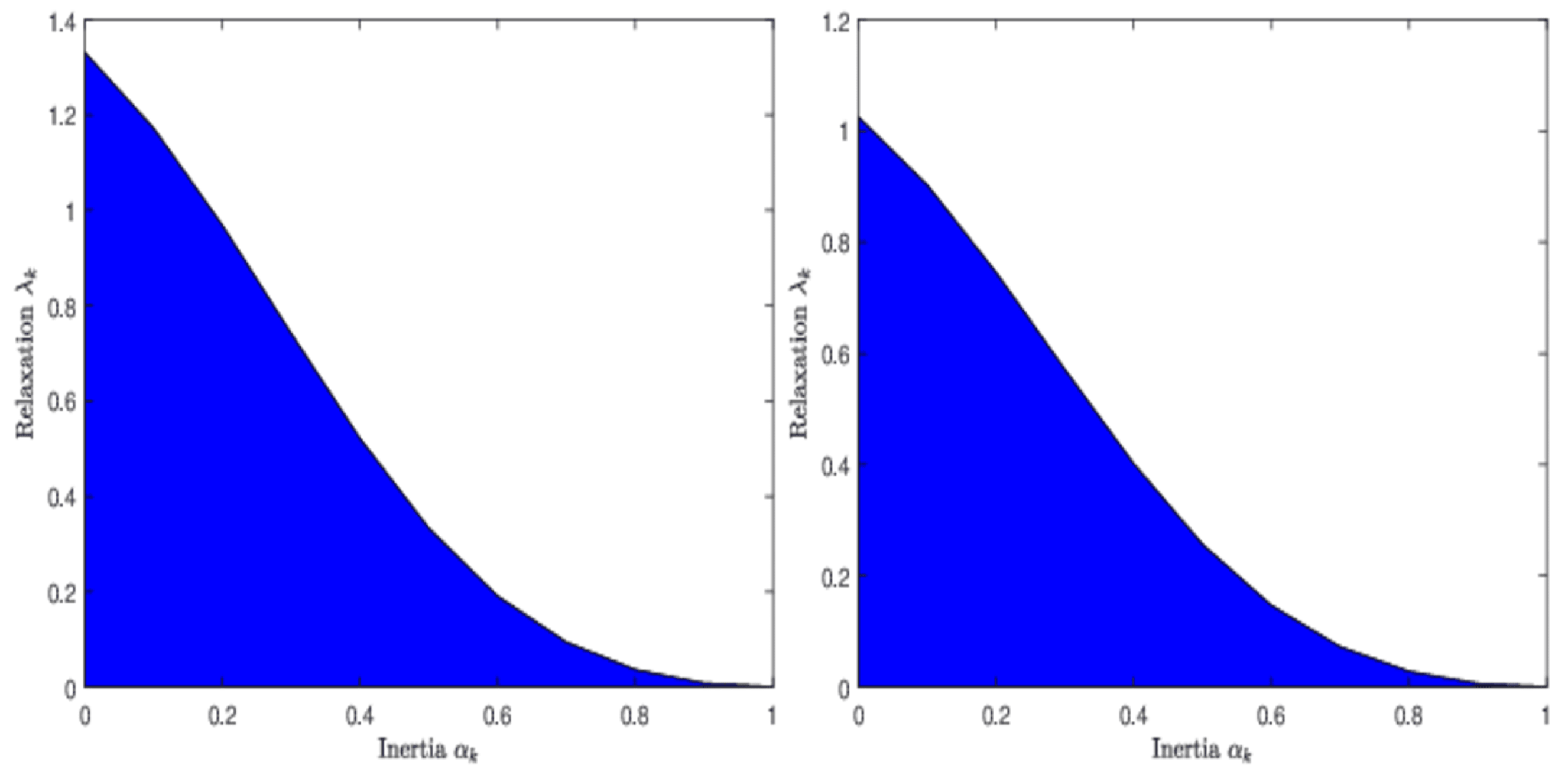
Remark 2

(Inertia versus relaxation). The inequation (19) establishes a relationship between inertial and relaxation parameters. Figure 1 displays the relationship between ${\alpha }_k$ and ${\lambda }_k$ by a graphical representation for some given values of γ and ε, which has a similar graphical representation to Figure 1 in [36]. It is noteworthy that the expression of the upper bound for ${\lambda }_k$ resembles that in ([36], Remark 2) if $\epsilon \searrow 0$. Assume that $\frac{2(1+\gamma L)-\epsilon }{{(1+\gamma L)}^2}$ is constant; it follows from (19) that the upper bound of ${\lambda }_k$ takes the form of ${\lambda }_{max}(\alpha ,\gamma )=\frac{2(1+\gamma L)-\epsilon }{{(1+\gamma L)}^2}\frac{{(1-\alpha )}^2}{(2{\alpha }^2-\alpha +1)}$ with $0\le \alpha <1$. Further, note that the relaxation parameter ${\lambda }_{max}(\alpha ,\gamma )$ is a decreasing function with respect to inertial parameter α on the interval $[0,1]$: for example, when $\alpha \nearrow 1$, then ${\lambda }_{max}(\alpha ,\gamma )\searrow 0$. Of course, we can also get ${\lambda }_{max}\left(\gamma \right)=\frac{2(1+\gamma L)-\epsilon }{{(1+\gamma L)}^2}$ when $\alpha =0$, and ${\lambda }_{max}\left(\gamma \right)$ is also decreasing on $(0,\frac{1}{L})$ because of limiting values $2-\epsilon$ as $\gamma \searrow 0$ and $1-\frac{\epsilon }{4}$ as $\gamma \nearrow \frac{1}{L}$.

Remark 3.

The parameters for FBHF [15] and RIFBHF are given in

Table 1. The parameter selection range for FBHF [15] and RIFBHF.

Algorithms	${\mathit{\gamma }}_{\mathit{k}}$	${\mathit{\alpha }}_{\mathit{k}}$	${lim}_{\mathit{k}\to +\mathit{\infty }}{\mathit{\lambda }}_{\mathit{k}}=\mathit{\lambda }$
FBHF [15]	$[\eta ,\chi -\eta ]$	0	1
RIFBHF	$[\eta ,\chi -\eta ]$	$[0,1)$	$\left(0,\frac{2(1+\gamma L)-\epsilon }{{(1+\gamma L)}^2}\frac{{(1-\alpha )}^2}{(2{\alpha }^2-\alpha +1)}\right)$

, which shows that the two schemes have the same range of step sizes. Different from FBHF [15], RIFBHF introduces relaxation parameter ${\lambda }_k$ and inertial parameter ${\alpha }_k$. Note that RIFBHF can reduce to FBHF [15] if ${\lambda }_k=1$ and ${\alpha }_k=0$.

Remark 4.

The existence of the over-relaxation $({\lambda }_k>1)$ for RIFBHF deserves further discussion. If $0\le \alpha <\frac{\sqrt{{\theta }^2+4(2{\gamma }^2{L}^2+2\gamma L+\epsilon )(1-\epsilon -{\gamma }^2{L}^2)}-\theta }{2(2{\gamma }^2{L}^2+2\gamma L+\epsilon )}$ with $\theta =2\gamma L-{\gamma }^2{L}^2+3-2\epsilon$ for $k\ge k_0$, we conclude that ${\lambda }_k$ has over-relaxation. In addition, observe that the over-relaxation in [36] exists when $0\le \alpha <\frac{\sqrt{{(3-\gamma L)}^2+8\gamma L(1-\gamma L)}-3+\gamma L}{4\gamma L}$ for $k\ge k_0$. Although the upper bounds of α for the two approaches are different, the over-relaxation $({\lambda }_k>1)$ for the two methods is possible when α is in a small range.

4. Composite Monotone Inclusion Problem

The aim of this section is to use the proposed algorithm to solve a more generalized inclusion problem, which is outlined as follows:

$$0\in Ax+L^{*}BLx+Cx,$$

(25)

where $A:\mathcal{H}\to 2^{\mathcal{H}}$ and $B:\mathcal{G}\to 2^{\mathcal{G}}$ represent two maximal monotone operators, $C:\mathcal{H}\to \mathcal{H}$ is a $\beta$-cocoercive operator with $\beta >0$, and $L:\mathcal{H}\to \mathcal{G}$ is a bounded linear operator. In addition, the following assumption is given:

$$\mathrm{zer}(A+L^{*}BL+C)\ne Ø.$$

The key to solving (25) is to know the exact resolvent $J_{L^{*}BL}$. As we know, $J_{L^{*}BL}$ can be estimated exactly using only the resolvent of the operator B, the linear operator L, and its adjoint $L^{*}$ when $L^{*}L=\nu I$ for some $\nu >0$. However, this condition usually does not hold in our interesting problems, such as total variation regularization. To address this challenge, we introduce an efficient iterative algorithm to tackle (25) by combining the primal–dual approach [39] and (6). Specifically, drawing inspiration from the fully splitting primal–dual algorithm studied by Briceño-Arias and Combettes [39], we naturally rewrite (25) as the following problem, letting $\mathcal{K}=\mathcal{H}⨁\mathcal{G}$:

$$\mathrm{find}x\in \mathcal{K}\mathrm{such}\mathrm{that}0\in Mx+Sx+Nx,$$

(26)

where

$$\left\{\begin{array}{c}M:\mathcal{K}\to 2^{\mathcal{K}}:(x,y)\mapsto \left(Ax\right)\times \left(B^{-1}y\right),\hfill \\ S:\mathcal{K}\to \mathcal{K}:(x,y)\mapsto (L^{*}y,-Lx),\hfill \\ N:\mathcal{K}\to \mathcal{K}:(x,y)\mapsto (Cx,0).\hfill \end{array}\right.$$

(27)

Notice that M is maximal monotone and S is monotone Lipschitz continuous within a constant $\parallel L\parallel$, as stated in Proposition 2.7 of [39]. This implies that $M+S$ is also maximal monotone since S is skew-symmetric. A result yields the cocoercivity of N by the cocoercivity of C. Therefore, it follows from (6) and (27) that the following convergence analysis can deal with (26), which implies that (25) is also solved.

Corollary 1.

Suppose that $A:\mathcal{H}\to 2^{\mathcal{H}}$ is maximal monotone; let $B:\mathcal{G}\to 2^{\mathcal{G}}$ be maximal monotone, and assume that $C:\mathcal{H}\to \mathcal{H}$ is β-cocoercive with $\beta >0$. Let $L:\mathcal{H}\to \mathcal{G}$ be a nonzero bounded linear operator. Given initial data $x_0,x_1\in \mathcal{H}$ and $y_0,y_1\in \mathcal{G}$, the iteration sequences are defined:

$$⌊\begin{array}{c}{w}_{1,k}=x_k+{\alpha }_k(x_k-x_{k-1}),\hfill \\ w_{2,k}=y_k+{\alpha }_k(y_k-y_{k-1}),\hfill \\ z_{1,k}=J_{{\gamma }_{k}A}(w_{1,k}-{\gamma }_k(L^{*}{w}_{2,k}+C{w}_{1,k})),\hfill \\ z_{2,k}=J_{{\gamma }_k{B}^{-1}}(w_{2,k}+{\gamma }_{k}L{w}_{1,k}),\hfill \\ t_{1,k}=z_{1,k}+{\gamma }_k(L^{*}{w}_{2,k}-L^{*}{z}_{2,k}),\hfill \\ t_{2,k}=z_{2,k}+{\gamma }_k(-L{w}_{1,k}+L{z}_{1,k}),\hfill \\ x^{k+1}=(1-{\lambda }_k)w_{1,k}+{\lambda }_k{t}_{1,k},\hfill \\ y^{k+1}=(1-{\lambda }_k)w_{2,k}+{\lambda }_k{t}_{2,k},\hfill \end{array}$$

(28)

where $\eta \le {\gamma }_k\le \chi -\eta$, $0<\eta <\frac{\chi }{2}$, χ is defined in Proposition 1, and ${\left\{{\alpha }_k\right\}}_{k\ge 1}$ is non-decreasing such that $0\le {\alpha }_k\le \alpha <1$. Assume that the sequence ${\left\{{\lambda }_k\right\}}_{k\ge 1}$ fulfils the condition

$$0<\underset{k\to +\infty }{lim}{\lambda }_k=\lambda <\frac{2(1+\gamma \parallel L\parallel )-\epsilon }{{(1+\gamma \parallel L\parallel )}^2}\frac{{(1-\alpha )}^2}{(2{\alpha }^2-\alpha +1)},$$

where $\epsilon =\frac{2}{1+\sqrt{1+16{\beta }^2{\parallel L\parallel }^2}}$. Therefore, the iterative sequence ${\left\{x_k\right\}}_{k\ge 1}$ generated by (28) weakly converges to a solution of $zer(A+L^{*}BL+C)$.

Proof. 

Using Proposition 2.7 in [39], we observe that M is maximal monotone and S is Lipschitz continuous together with $\parallel L\parallel$. Considering the $\beta$-cocoercivity of C, it follows that N is also $\beta$-cocoercive. Additionally, for arbitrary $k\ge 1$, let

$$\left\{\begin{array}{c}{x}_k=(x_k,y_k),\hfill \\ w_k=(w_{1,k},w_{2,k}),\hfill \\ z_k=(z_{1,k},z_{2,k}),\hfill \\ t_k=(t_{1,k},t_{2,k}).\hfill \end{array}\right.$$

Therefore, using (27) and Proposition 2.7 (iv) in [39], we can rewrite (28) in the following form:

$$\left\{\begin{array}{c}{w}_k=x_k+{\alpha }_k(x_k-x_{k-1}),\hfill \\ z_k=J_{{\gamma }_{k}M}(w_k-{\gamma }_k(S+N)w_k),\hfill \\ t_k=z_k+{\gamma }_k(S{w}_k-S{z}_k),\hfill \\ x_{k+1}=(1-{\lambda }_k)w_k+{\lambda }_k{t}_k,\hfill \end{array}\right.$$

which has the same structure as (6). Meanwhile, our assumptions guarantee that the conditions of Theorem 1 are held. Hence, according to Theorem 1, the sequence ${\left\{x_k\right\}}_{k\ge 1}$ generated by (28) weakly converges to an element of $\mathrm{zer}(A+L^{*}BL+C)$. □

In the following, we apply the results of Corollary 1 to tackle the convex minimization problem.

Corollary 2.

Consider the convex optimization problem as follows:

$$\underset{x\in \mathcal{H}}{min}f\left(x\right)+g\left(Lx\right)+h\left(x\right),$$

(29)

where $f\in {\Gamma }_0\left(\mathcal{H}\right)$, $g\in {\Gamma }_0\left(\mathcal{G}\right)$, $h:\mathcal{H}\to \mathbb{R}$ is convex differentiable with $\frac{1}{\beta }$-Lipschitz continuous gradient for some $\beta >0$, and $L:\mathcal{H}\to \mathcal{G}$ is a bounded linear operator. For (29), given initial data $x_0,x_1\in \mathcal{H}$ and $y_0,y_1\in \mathcal{G}$, iteration sequences are presented for $k\ge 1$:

$$⌊\begin{array}{c}{w}_{1,k}=x_k+{\alpha }_k(x_k-x_{k-1}),\hfill \\ w_{2,k}=y_k+{\alpha }_k(y_k-y_{k-1}),\hfill \\ z_{1,k}={\mathrm{prox}}_{{\gamma }_{k}f}(w_{1,k}-{\gamma }_k(L^{*}{w}_{2,k}+\nabla h\left(w_{1,k}\right))),\hfill \\ z_{2,k}={\mathrm{prox}}_{{\gamma }_k{g}^{*}}(w_{2,k}+{\gamma }_{k}L{w}_{1,k}),\hfill \\ t_{1,k}=z_{1,k}+{\gamma }_k(L^{*}{w}_{2,k}-L^{*}{z}_{2,k}),\hfill \\ t_{2,k}=z_{2,k}+{\gamma }_k(-L{w}_{1,k}+L{z}_{1,k}),\hfill \\ x_{k+1}=(1-{\lambda }_k)w_{1,k}+{\lambda }_k{t}_{1,k},\hfill \\ y_{k+1}=(1-{\lambda }_k)w_{2,k}+{\lambda }_k{t}_{2,k},\hfill \end{array}$$

(30)

where $\eta \le {\gamma }_k\le \chi -\eta$, $0<\eta <\frac{\chi }{2}$, χ is defined in Proposition 1, and ${\left\{{\alpha }_k\right\}}_{k\ge 1}$ is nondecreasing such that $0\le {\alpha }_k\le \alpha <1$. Assume that the sequence ${\left\{{\lambda }_k\right\}}_{k\ge 1}$ satisfies that

$$0<\underset{k\to +\infty }{lim}{\lambda }_k=\lambda <\frac{2(1+\gamma \parallel L\parallel )-\epsilon }{{(1+\gamma \parallel L\parallel )}^2}\frac{{(1-\alpha )}^2}{(2{\alpha }^2-\alpha +1)},$$

where $\epsilon =\frac{2}{1+\sqrt{1+16{\beta }^2{\parallel L\parallel }^2}}$. If $\mathrm{zer}(\partial f+L^{*}\circ \partial g\circ L+\nabla h)$ is nonempty, then the sequence ${\left\{x_k\right\}}_{k\ge 1}$ weakly converges to a minimizer of (29).

Proof. 

According to [4], $\partial f$ and $\partial g$ are maximal monotone. In view of the Baillon–Haddad theorem, $\nabla h$ is indicated to be $\beta$-cocoercive. Thus, solving (29) with our algorithm is equivalent to (25) under suitable qualification conditions, which gives

$$A=\partial f,B=\partial g\mathrm{a}\mathrm{n}\mathrm{d}C=\nabla h.$$

Therefore, it follows from the same arguments as the proof of Corollary 1 that we arrive at the conclusions of Corollary 2. □

5. Numerical Experiments

This section reports the feasibility and efficiency of (6). In particular, we discuss the impact of parameters on (6). All experiments were conducted using MATLAB on a standard Lenovo machine equipped with an Intel(R) Core(TM) i5-8265U CPU @ 1.60 GHz with 1.80 GHz boost. Our objective is to address the following constrained total variation (TV) minimization problem:

$$\underset{z\in D}{min}\frac{1}{2}{\parallel Az-d\parallel }_2^2+\mu {\parallel z\parallel }_{TV},$$

(31)

in which $A\in {\mathbb{R}}^{m\times n}$ represents the blurring matrix, z signifies the unknown original image in ${\mathbb{R}}^{n^2}$, and D indicates a nonempty closed convex set and represents the prior information regarding the deblurred images. Specifically, D is selected as a nonnegative constraint set, $\mu >0$ indicates the regularization parameter, ${\parallel z\parallel }_{TV}$ denotes the total variation term, and d stands for the recorded blurred image data.

Notice that (31) can be equivalently written with the following structure:

$$\underset{z}{min}\frac{1}{2}{\parallel Az-d\parallel }_2^2+\mu {\parallel z\parallel }_{TV}+{\delta }_D\left(z\right),$$

(32)

where ${\delta }_D\left(z\right)$ represents the indicator function, which equals 0 when $z\in D$ and $+\infty$ otherwise. The term ${\parallel z\parallel }_{TV}$ can be expressed as a combination of a convex function $\phi$ (either using ${\parallel ·\parallel }_1$ for the anisotropic total-variation or ${\parallel ·\parallel }_2$ for the isotropic total-variation) with a first-order difference matrix H, denoted as ${\parallel z\parallel }_{TV}=\phi \left(Hz\right)$ (refer to Section 4 in [41]), where H represents a $2n^2\times n^2$ matrix written as:

$$\begin{array}{c}H:=\left[\begin{array}{c}{I}_n⨂E\\ E⨂I_n\end{array}\right]\mathrm{and}E:={\left[\begin{array}{cccc}0& & & \\ -1& 1& & \\ & \ddots & \ddots & \\ & & -1& 1\end{array}\right]}_{n\times n},\end{array}$$

where $I_n$ denotes the $n\times n$ identity matrix, and ⨂ is the Kronecker product. Consequently, it is evident that (32) constitutes a special instance of (29).

In order to assess the quality of the deblurred images, we employ the signal-to-noise ratio (SNR) [40], which is defined by

$$SNR=10log\frac{{\parallel x\parallel }^2}{\parallel x-x_r{\parallel }^2},$$

where x is the original image, and $x_r$ is the deblurred image. The following stopping criterion is utilized to terminate iterative algorithms by the relative error between adjacent iterative steps. We choose test image “Barbara" with a size of $512\times 512$ and use four typical image blurring scenarios as in

Table 2. Description of image blurring scenarios.

Scenario	Blur Kernel	Gaussian Noise
1	$9\times 9$ box average kernel	$\sigma =1.5$
2	$9\times 9$ box average kernel	$\sigma =3$
3	$7\times 7$ Gaussian kernel with ${\sigma }_a=10$	$\sigma =1.5$
4	$7\times 7$ Gaussian kernel with ${\sigma }_a=10$	$\sigma =3$

. In addition, the range of the values in the original images is $[0,255]$, and the norm of operator A in (31) is equal to 1 for the selected experiments. The cocoercive coefficient $\beta$ is 1, and ${\parallel H\parallel }^2=8$ for the total variation, as estimated in [41], where H is the linear operator. We terminate the iterative algorithms if the relative error is less than $5\times {10}^{-4}$ or if the maximum number of iterations reaches 1000.

Prior to the comparisons, we do a test to display how the performance of RIFBHF is affected by different parameters. For simplicity, we set ${\gamma }_k=\gamma$ for all $k\ge 1$. In view of (19), the relationship between inertial parameter $\alpha$ and relaxation parameter $\lambda$ is presented as follows:

$$0<\underset{k\to +\infty }{lim}{\lambda }_k=\lambda <\frac{2(1+\gamma \parallel L\parallel )-\epsilon }{{(1+\gamma \parallel L\parallel )}^2}\frac{{(1-\alpha )}^2}{(2{\alpha }^2-\alpha +1)},$$

where $0\le \alpha <1$, and $\epsilon =\frac{2}{1+\sqrt{1+16{\beta }^2{\parallel L\parallel }^2}}$. As we know, the upper boundedness of $\lambda$ is similar to the one of ([36], Remark 2) if $\epsilon \searrow 0$. Firstly, we assume $\gamma =\frac{4\beta }{1+\sqrt{1+16{\beta }^2{L}^2}}$, $\alpha =0$, and $\lambda =1$, or $\alpha =0.3$ and $\lambda =0.6$ for RIFBHF. The SNR values and the numbers of iterations used with various $\mu$ for RIFBHF are recorded in

Table 3. SNR values and iterations when $\gamma =\frac{4}{1+\sqrt{1+16\ast 8}}$, $\alpha =0$, and $\lambda =1$ with different parameter $\mu$ for Barbara image in four blurred scenarios.

	Scenario	1		2		3		4
$\mathit{\mu }$		SNR (dB)	Iter	SNR (dB)	Iter	SNR (dB)	Iter	SNR (dB)	Iter
$0.1$		$17.5358$	50	$17.5144$	52	$17.9741$	45	$17.9510$	48
$0.5$		$17.5414$	55	$17.5196$	56	$17.9385$	49	$17.9148$	51
1		$17.5515$	61	$17.5304$	62	$17.9071$	54	$17.8799$	55
2		$17.4859$	65	$17.4658$	65	$17.8012$	56	$17.7788$	57
3		$17.4001$	65	$17.3831$	65	$17.7126$	56	$17.6937$	57
4		$17.3251$	65	$17.3106$	66	$17.6368$	57	$17.6203$	57
5		$17.2584$	67	$17.2443$	68	$17.5713$	58	$17.5553$	59
6		$17.1948$	69	$17.1823$	69	$17.5117$	60	$17.4972$	60
7		$17.1344$	71	$17.1230$	71	$17.4563$	61	$17.4422$	62
8		$17.0779$	73	$17.0663$	74	$17.4033$	63	$17.3895$	64
9		$17.0237$	75	$17.0123$	76	$17.3530$	65	$17.3413$	65
10		$16.9718$	77	$16.9608$	78	$17.3049$	67	$17.2940$	67

and

Table 4. SNR values and iterations when $\gamma =\frac{4}{1+\sqrt{1+16\ast 8}}$, $\alpha =0.3$, and $\lambda =0.6$ with different parameter $\mu$ for Barbara image in four blurred scenarios.

	Scenario	1		2		3		4
$\mathit{\mu }$		SNR (dB)	Iter	SNR (dB)	Iter	SNR (dB)	Iter	SNR (dB)	Iter
$0.1$		$17.4757$	52	$17.4513$	53	$17.9109$	46	$17.8957$	49
$0.5$		$17.4740$	55	$17.4573$	56	$17.8890$	50	$17.8643$	51
1		$17.5060$	62	$17.4884$	63	$17.8783$	56	$17.8545$	57
2		$17.4687$	68	$17.4502$	68	$17.7913$	59	$17.7707$	60
3		$17.3929$	69	$17.3785$	70	$17.7093$	60	$17.6920$	61
4		$17.3214$	70	$17.3072$	70	$17.6367$	61	$17.6212$	61
5		$17.2577$	72	$17.2446$	72	$17.5723$	62	$17.5582$	63
6		$17.1970$	74	$17.1850$	75	$17.5144$	64	$17.5007$	65
7		$17.1384$	76	$17.1277$	76	$17.4600$	66	$17.4480$	66
8		$17.0832$	78	$17.0725$	79	$17.4078$	68	$17.3953$	69
9		$17.0298$	81	$17.0203$	81	$17.3580$	70	$17.3463$	71
10		$16.9787$	83	$16.9686$	84	$17.3103$	72	$17.3005$	72

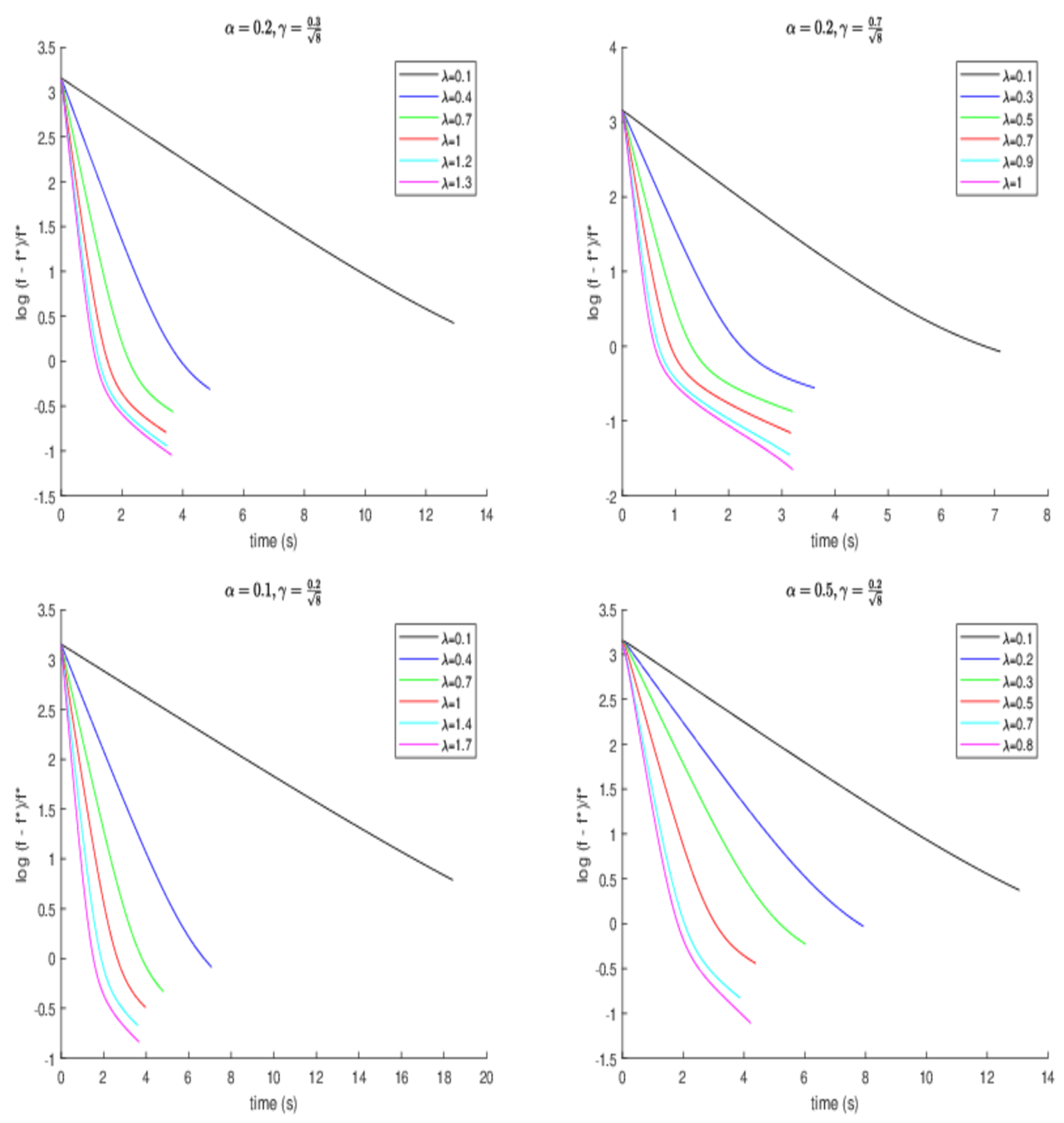
. Observe that the SNR values in image blurring scenarios 1 and 2 are the best when $\mu =1$, while the SNR values in image blurring scenarios 3 and 4 are the best when $\mu =0.1$. Therefore, we choose $\mu =1$ for image blurring scenarios 1 and 2 and $\mu =0.1$ for image blurring scenarios 3 and 4. For the case of $\mu =1$ in image blurring scenario 1, we further study the effect of the other parameters. The development of the SNR value and the normalized error of the objective function $log(f-f^{*})/f^{*}$ along the running time are considered; here, f represents the present objective value, while $f^{*}$ signifies the optimal objective value. To obtain an approximation of the optimal objective value, we set the function value given by running experimental algorithms for 5000 iterations as an estimate of the optimal value. One can observe that a larger $\gamma$ results in better error when $\alpha =0.2$ and $\lambda =0.7$, and a larger $\alpha$ also brings better error when $\gamma =\frac{0.2}{\sqrt{8}}$ and $\lambda =0.7$ in Figure 2. Of course, $\alpha$ and $\gamma$ also affect the value of $\lambda$. Meanwhile, a conclusion that a larger $\lambda$ allows for better error can be given. It is worth noting that over-relaxation ($\lambda >1$) exists, and it enjoys a better effect. 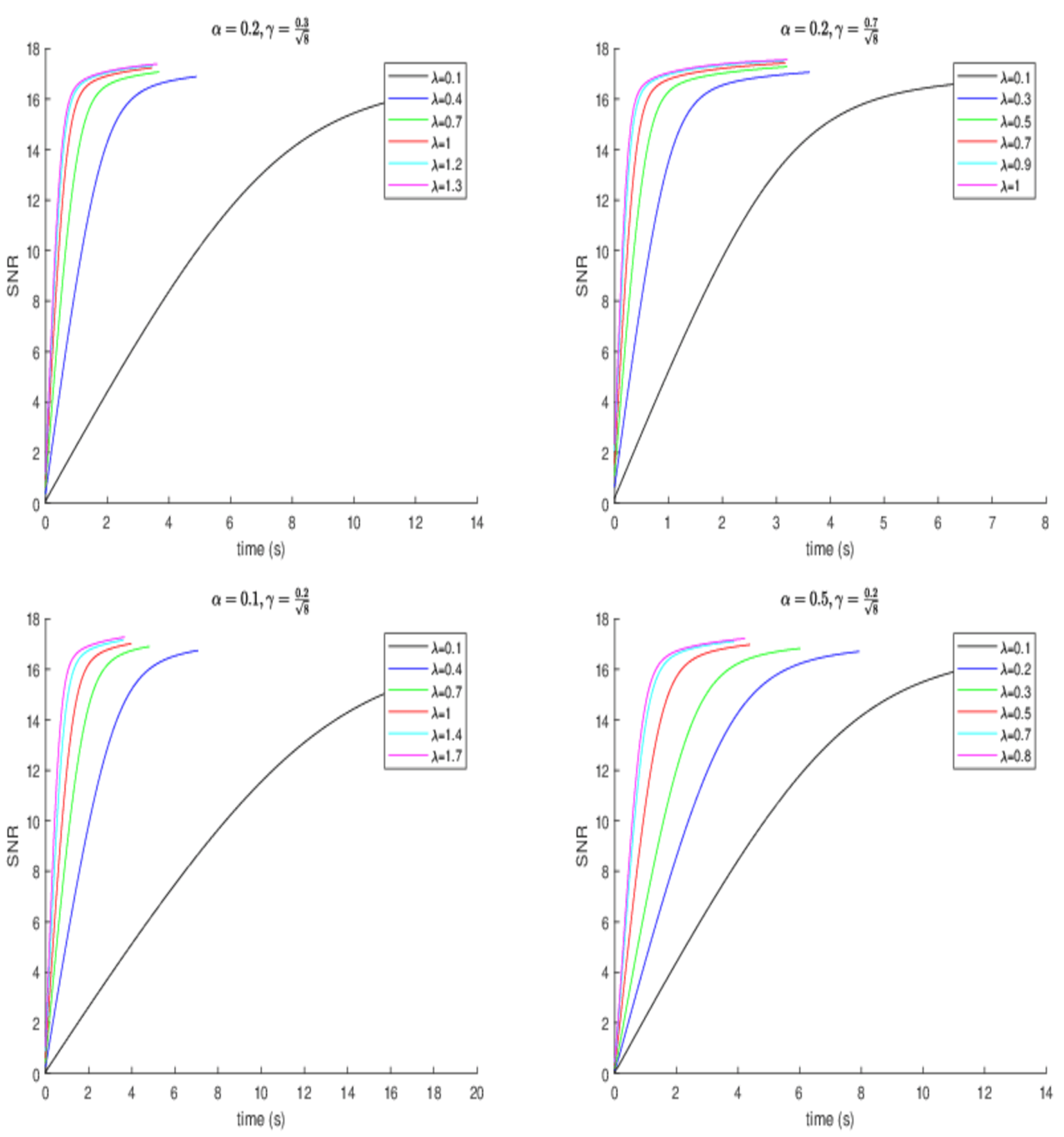Figure 3 shows the development of SNR for different parameters; the experiment results are similar to those in Figure 2.

To further validate the rationality and efficiency of (30), the following algorithms and parameter settings are utilized:

• FBHF [15]: $\gamma =\frac{4\beta }{1+\sqrt{1+16{\beta }^2{L}^2}}$ for four image blurring scenarios.
• PD: the first-order primal–dual splitting algorithm [42] with $\tau =\frac{1}{3}$, $\sigma =\frac{1}{3}$, and $\theta =1$ for four image blurring scenarios.
• RIFBHF: $\gamma =\frac{4\beta }{1+\sqrt{1+16{\beta }^2{L}^2}}$ using $\alpha =0.2$ and $\lambda =0.9$ for image blurring scenarios 1 and 2 and $\alpha =0.6$ and $\lambda =0.8$ for image blurring scenarios 3 and 4.

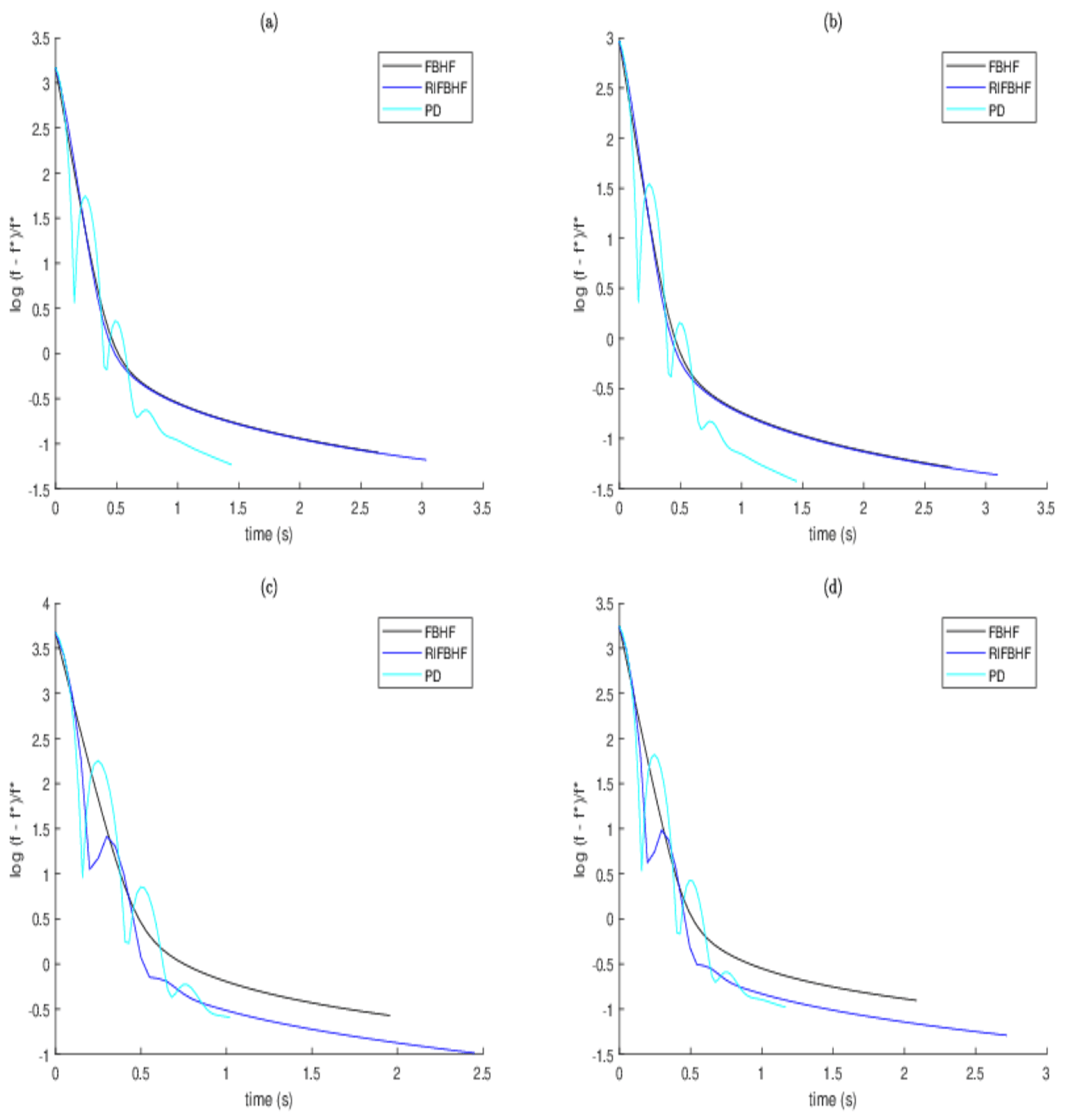
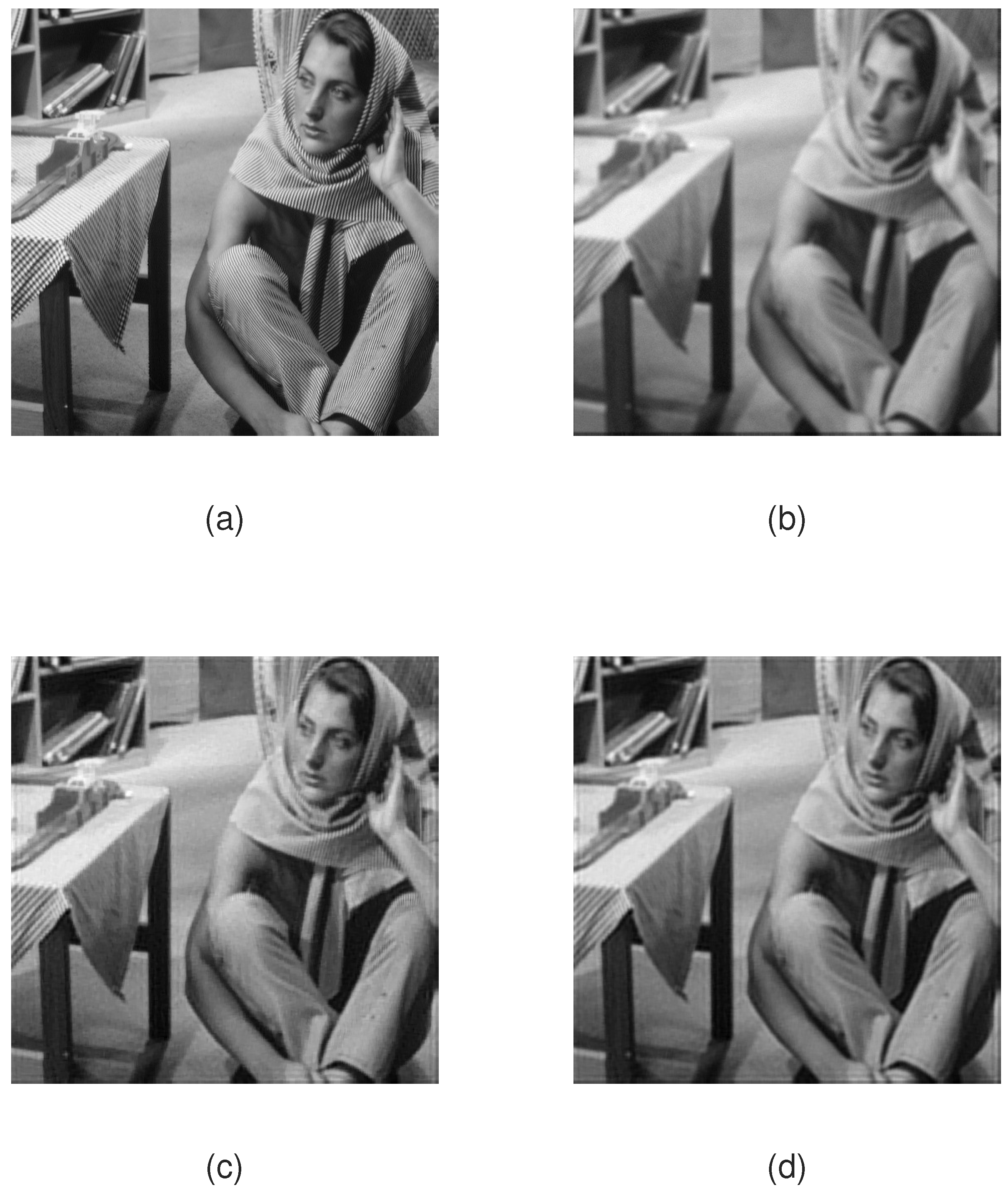
Figure 4 plots the normalized error of the objective function of FBHF, PD, and RIFBHF along the running time. Note that PD appears to be the fastest algorithm. FBHF and RIFBHF are almost the same in image blurring scenarios 1 and 2, while in image blurring scenarios 3 and 4, the effect of RIFBHF is better than that of FBHF, which shows that our algorithm is acceptable. Meanwhile, to succinctly illustrate the deblurring impact of the proposed algorithm, the deblurred results of image blurring scenario 4 are shown in Figure 5. One can observe visually the better deblurred images generated by RIFBHF.

6. Conclusions

In this paper, we proposed an RIFBHF algorithm to solve (1). On the way, the proposed approach was deduced by discretising a continuous-time dynamical system, and a variable stepsize was introduced into the proposed algorithm. Additionally, we studied the theoretical convergence properties of (6) under reasonable parameter conditions. Inspired by the primal–dual scheme, our approach tackled both the composite monotone inclusion problem (25) and analysed the composite convex optimization problem (29). Subsequently, we conducted numerical experiments focused on image deblurring to illustrate the effectiveness of our proposed technique.

References

1. Daubechies, I.; Defrise, M.; De Mol, C. An iterative thresholding algorithm for linear inverse problems with a sparsity constraint. Comm. Pure Appl. Math. 2004, 57, 1413–1457. [Google Scholar] [CrossRef]
2. Combettes, P.L.; Wajs, V.R. Signal recovery by proximal forward-backward splitting. Multiscale Model. Simul. 2005, 4, 1168–1200. [Google Scholar] [CrossRef]
3. Raguet, H.; Fadili, J.; Peyré, G. A generalized forward-backward splitting. SIAM J. Imaging Sci. 2013, 6, 1199–1226. [Google Scholar] [CrossRef]
4. Bauschke, H.H.; Combettes, P.L. Convex Analysis and Monotone Operator Theory in Hilbert Spaces; Springer: London, UK, 2017. [Google Scholar]
5. Goldstein, A.A. Convex programming in Hilbert space. Bull. Am. Math. Soc. 1964, 70, 709–710. [Google Scholar] [CrossRef]
6. Lions, P.-L.; Mercier, B. Splitting algorithms for the sum of two nonlinear operators. SIAM J. Numer. Anal. 1979, 16, 964–979. [Google Scholar] [CrossRef]
7. Combettes, P.L.; Pesquet, J.-C. A Douglas-Rachford splitting approach to nonsmooth convex variational signal recovery. IEEE J. Sel. Top. Signal Process. 2007, 1, 564–574. [Google Scholar] [CrossRef]
8. Tseng, P. A modified forward-backward splitting method for maximal monotone mappings. SIAM J. Control Optim. 2000, 38, 431–446. [Google Scholar] [CrossRef]
9. Raguet, H.; Landrieu, L. Preconditioning of a generalized forward-backward splitting and application to optimization on graphs. SIAM J. Imaging Sci. 2015, 8, 2706–2739. [Google Scholar] [CrossRef]
10. Briceño-Arias, L.M. Forward-Douglas-Rachford splitting and forward-partial inverse method for solving monotone inclusions. Optimization 2015, 64, 1239–1261. [Google Scholar] [CrossRef]
11. Davis, D.; Yin, W.T. A three-operator splitting scheme and its optimization applications. Set-Valued Var. Anal. 2017, 25, 829–858. [Google Scholar] [CrossRef]
12. Raguet, H. A note on the forward-Douglas-Rachford splitting for monotone inclusion and convex optimization. Optim. Lett. 2019, 13, 717–740. [Google Scholar] [CrossRef]
13. Ryu, E.K.; Vũ, B.C. Finding the forward-Douglas-Rachford-forward method. J. Optim. Theory Appl. 2020, 184, 858–876. [Google Scholar] [CrossRef]
14. Rieger, J.; Tam, M.K. Backward-forward-reflected-backward splitting for three operator monotone inclusions. Appl. Math. Comput. 2020, 381, 125248. [Google Scholar] [CrossRef]
15. Briceño-Arias, L.M.; Davis, D. Forward-backward-half forward algorithm for solving monotone inclusions. SIAM J. Optim. 2018, 28, 2839–2871. [Google Scholar] [CrossRef]
16. Alves, M.M.; Geremia, M. Iteration complexity of an inexact Douglas-Rachford method and of a Douglas-Rachford-Tseng’s F-B four-operator splitting method for solving monotone inclusions. Numer. Algorithms 2019, 82, 263–295. [Google Scholar] [CrossRef]
17. Giselsson, P. Nonlinear forward-backward splitting with projection correction. SIAM J. Optim. 2021, 31, 2199–2226. [Google Scholar] [CrossRef]
18. Briceño-Arias, L.; Chen, J.; Roldán, F.; Tang, Y. Forward-partial inverse-half-forward splitting algorithm for solving monotone inclusions. Set-Valued Var. Anal. 2022, 30, 1485–1502. [Google Scholar] [CrossRef]
19. Polyak, B.T. Some methods of speeding up the convergence of iteration methods. USSR Comput. Math. Math. Phys. 1964, 4, 1–17. [Google Scholar] [CrossRef]
20. Nesterov, Y. A method for unconstrained convex minimization problem with the rate of convergence O( 1 k 2 ). Doklady AN SSSR 1983, 269, 543–547. [Google Scholar]
21. Güler, O. New proximal point algorithms for convex minimization. SIAM J. Optim. 1992, 2, 649–664. [Google Scholar] [CrossRef]
22. Alvarez, F.; Attouch, H. An inertial proximal method for maximal monotone operators via discretization of a nonlinear oscillator with damping. Set-Valued Anal. 2001, 9, 3–11. [Google Scholar] [CrossRef]
23. Alvarez, F. Weak convergence of a relaxed and inertial hybrid projection-proximal point algorithm for maximal monotone operators in Hilbert space. SIAM J. Optim. 2003, 14, 773–782. [Google Scholar] [CrossRef]
24. Ochs, P.; Chen, Y.; Brox, T.; Pock, T. iPiano: Inertial proximal algorithm for nonconvex optimization. SIAM J. Imaging Sci. 2014, 7, 1388–1419. [Google Scholar] [CrossRef]
25. Boţ, R.I.; Csetnek, E.R. A hybrid proximal-extragradient algorithm with inertial effects. Numer. Funct. Anal. Optim. 2015, 36, 951–963. [Google Scholar] [CrossRef]
26. Chen, C.; Chan, R.H.; Ma, S.; Yang, J. Inertial proximal ADMM for linearly constrained separable convex optimization. SIAM J. Imaging Sci. 2015, 8, 2239–2267. [Google Scholar] [CrossRef]
27. Dong, Q.; Lu, Y.; Yang, J. The extragradient algorithm with inertial effects for solving the variational inequality. Optimization 2016, 65, 2217–2226. [Google Scholar] [CrossRef]
28. Combettes, P.L.; Glaudin, L.E. Quasi-nonexpansive iterations on the affine hull of orbits: From Mann’s mean value algorithm to inertial methods. SIAM J. Optim. 2017, 27, 2356–2380. [Google Scholar] [CrossRef]
29. Attouch, H.; Cabot, A. Convergence rates of inertial forward-backward algorithms. SIAM J. Optim. 2018, 28, 849–874. [Google Scholar] [CrossRef]
30. Eckstein, J.; Bertsekas, D.P. On the Douglas-Rachford splitting method and the proximal point algorithm for maximal monotone operators. Math. Program. 1992, 55, 293–318. [Google Scholar] [CrossRef]
31. Attouch, H.; Peypouquet, J. Convergence of inertial dynamics and proximal algorithms governed by maximally monotone operators. Math. Program. 2019, 174, 391–432. [Google Scholar] [CrossRef]
32. Attouch, H.; Cabot, A. Convergence of a relaxed inertial proximal algorithm for maximally monotone operators. Math. Program. 2020, 184, 243–287. [Google Scholar] [CrossRef]
33. Attouch, H.; Cabot, A. Convergence rate of a relaxed inertial proximal algorithm for convex minimization. Optimization 2020, 69, 1281–1312. [Google Scholar] [CrossRef]
34. Attouch, H.; Cabot, A. Convergence of a relaxed inertial forward-backward algorithm for structured monotone inclusions. Appl. Math. Optim. 2019, 80, 547–598. [Google Scholar] [CrossRef]
35. Boţ, R.I.; Csetnek, E.R.; Hendrich, C. Inertial Douglas-Rachford splitting for monotone inclusion problems. Appl. Math. Comput. 2015, 256, 472–487. [Google Scholar] [CrossRef]
36. Boţ, R.I.; Sedlmayer, M.; Vuong, P.T. A relaxed inertial forward-backward-forward algorithm for solving monotone inclusions with application to GANs. J. Mach. Learn. Res. 2023, 1–37. [Google Scholar]
37. Tang, Y.; Yang, Y.; Peng, J. Convergence analysis of a relaxed inertial alternating minimization algorithm with applications. In Advanced Mathematical Analysis and Its Applications, 1st ed.; Chapman and Hall/CRC: Boca Raton, FL, USA, 2023; 27p. [Google Scholar]
38. Boţ, R.I.; Csetnek, E.R. Second order forward-backward dynamical systems for monotone inclusion problems. SIAM J. Control Optim. 2016, 54, 1423–1443. [Google Scholar] [CrossRef]
39. Briceño-Arias, L.M.; Combettes, P.L. A monotone+skew splitting model for composite monotone inclusions in duality. SIAM J. Optim. 2011, 21, 1230–1250. [Google Scholar] [CrossRef]
40. Zong, C.; Tang, Y.; Zhang, G. An accelerated forward-backward-half forward splitting algorithm for monotone inclusion with applications to image restoration. Optimization 2024, 73, 401–428. [Google Scholar] [CrossRef]
41. Micchelli, C.A.; Shen, L.; Xu, Y. Proximity algorithms for image models: Denoising. Inverse Problems 2011, 27, 045009. [Google Scholar] [CrossRef]
42. Chambolle, A.; Pock, T. A first-order primal-dual algorithm for convex problems with applications to imaging. J. Math. Imaging Vision 2011, 40, 120–145. [Google Scholar] [CrossRef]
Figure 1. Balance between α k and λ k with ε = 0.1 , γ = 0.45 L (left), and γ = 0.9 L (right).
Symmetry 16 00466 g001
Figure 2. Behaviour of the error of objective value log ( f f * ) / f * against running time for different parameters α , γ , and λ .
Symmetry 16 00466 g002
Figure 3. Behaviour of SNR against running time for different parameters α , γ , and λ .
Symmetry 16 00466 g003
Figure 4. Behaviour of the error of objective value log ( f f * ) / f * against running time for different image burring scenarios, i.e., (a) scenario 1, (b) scenario 2, (c) scenario 3, and (d) scenario 4.
Symmetry 16 00466 g004
Figure 5. (a) The original image of Barbara. (b) The blurred image of Barbara. (c) The deblurred image by FBHF. (d) The deblurred image by RIFBHF.
Symmetry 16 00466 g005