
Dynamics of a Stochastic SVEIR Epidemic Model with Nonlinear Incidence Rate
1
College of Science, Northwest A&F University, Yangling 712100, China
2
Department of Applied Mathematics, Lanzhou University of Technology, Lanzhou 730050, China
*
Author to whom correspondence should be addressed.
Symmetry 2024, 16(4), 467; https://doi.org/10.3390/sym16040467
Submission received: 11 March 2024
/
Revised: 4 April 2024
/
Accepted: 6 April 2024
/
Published: 11 April 2024
(This article belongs to the Special Issue Symmetry/Asymmetry of Differential Equations in Biomathematics)
Abstract
:This paper delves into the analysis of a stochastic epidemic model known as the susceptible–vaccinated–exposed–infectious–recovered (SVEIR) model, where transmission dynamics are governed by a nonlinear function. In the theoretical analysis section, by suitable stochastic Lyapunov functions, we establish that when the threshold value, denoted as , falls below 1, the epidemic is destined for extinction. Conversely, if the reproduction number of the deterministic model surpasses 1, the model manifests an ergodic endemic stationary distribution. In the numerical simulations and data interpretation section, leveraging a graphical analysis with COVID-19 data, we illustrate that random fluctuations possess the capacity to quell disease outbreaks, underscoring the role of vaccines in curtailing the spread of diseases. This study not only contributes to the understanding of epidemic dynamics but also highlights the pivotal role of stochasticity and vaccination strategies in epidemic control and management. The inherent balance and patterns observed in epidemic spread and control strategies, reflect a symmetrical interplay between stochasticity, vaccination, and disease dynamics.
1. Introduction
Over the past two decades, mathematical modeling has played a crucial role in both preventing and controlling infectious diseases, including severe acute respiratory syndrome (SARS) [1], human immunodeficiency virus infection/acquired immune deficiency syndrome (HIV/AIDS) [2], and H1N1 (swine flu) [3]. These models describe the evolution of various subpopulations over time within epidemic models. One widely used model is the SEIR (susceptible–exposed–infectious–recovered) model, which divides the population into four compartments: susceptible (S), individuals who are at risk of infection; exposed (E), individuals who have come into contact with infective individuals but show no symptoms; infectious (I), individuals displaying symptoms; and recovered (R), individuals who have recovered from the disease [4]. The SEIR model has various complex variants, including those with different control measures such as various incidence rates, constant and feedback vaccination and treatment controls, as well as models involving multiple interconnected regions or towns [5,6,7,8,9,10], and others cited within. The rate of incidence is widely recognized as playing a significant role in disease modeling, with factors such as population density and lifestyle influencing the increase and decrease in epidemics [11,12]. Many researchers have employed nonlinear incidence rates in their studies; for more in-depth information, readers are referred to [13,14,15,16,17,18,19] and related references. Vaccination is widely acknowledged as one of the most effective means of disease control and prevention [20], playing a pivotal role in the complete eradication of diseases like smallpox and partial control of diseases such as measles [21]. Numerous scholarly works have explored the dynamics of epidemic models with different vaccination schedules [7,13,19,22,23,24,25,26].
In 2018, Gao and Huang [22] conducted a study on the model described below:
All the parameters in model (1) are positive. The variables S, E, I, R, and V represent the respective counts of susceptible, exposed, infectious, recovered, and vaccinated individuals at time t. Table 1 provides the biological interpretations of the remaining parameters.
The results in [22] showed that the basic reproduction number of model (1) is
It is proved that if , the disease-free equilibrium is globally asymptotically stable and if , model (1) has an endemic equilibrium which is globally asymptotically stable.
The inherent randomness of epidemic growth and spread, attributed to the unpredictable nature of person-to-person contacts [27] and the susceptibility of populations to various disturbances [28], suggests that stochastic models may offer a more suitable approach for modeling epidemics in many scenarios [29,30,31,32,33,34,35,36,37,38,39,40,41,42]. Stochastic models are particularly beneficial in capturing the random occurrences of infectious contacts during the latent and infectious periods [43]. Many realistic stochastic epidemic models can be derived from their deterministic counterparts. For instance, Cai [38] developed a general SIRS epidemic model with a ratio-dependent incidence rate and its corresponding stochastic differential equation version. Ball and Neal [44] explored a general stochastic SIR model within a closed finite population, deriving a threshold parameter that determines the possibility of global epidemics. Yang et al. [45] examined the ergodicity and extinction of stochastic SIR and SEIR epidemic models with saturated incidence. Zhang and Zhang [42] investigated the threshold behavior of a deterministic and a stochastic SIQS epidemic model by considering varying total population sizes.
In its investigation of the stochastic epidemic model, our analysis not only sheds light on the dynamics of disease transmission and control but also unravels the symmetrical aspects inherent in epidemic behavior. By exploring the effects of stochasticity and vaccination strategies on disease spread, we can uncover a symmetrical relationship between these factors and the patterns observed in epidemic outcomes.
This paper focuses on a stochastic SVEIR epidemic model with a nonlinear incidence rate.
The parameters in model (1) remain unchanged, with denoting the intensities of white noise. Additionally, () represents independent standard Brownian motions, initialized at .
In the study of epidemic model behavior, analyzing steady states and their stability is crucial [19]. In deterministic models, this analysis involves examining the stability of the disease-free equilibrium (or endemic equilibrium) through the basic reproduction number . However, in the case of the stochastic model (3), there is no endemic equilibrium. Nevertheless, Khasminskii [46] demonstrated that the presence of an ergodic stationary distribution for model (3) can reveal the persistence of the infection.
The primary objective of this paper is to examine the extinction and the existence of an ergodic stationary distribution for model (3). We establish sufficient conditions for both the extinction and the existence of an ergodic stationary distribution.
The paper is organized as follows: Section 2 introduces the necessary preliminaries for subsequent analysis. Section 3 establishes sufficient conditions for both the extinction and the existence of an ergodic stationary distribution in model (3). Section 4 presents numerical simulations based on published data from COVID-19 to support our findings. Lastly, some concluding remarks summarize the results.
2. Preliminaries
Let be a complete probability space with a filtration satisfying the usual conditions, where it is increasing and right-continuous, and contains all P-null sets. Additionally, define .
We consider the d-dimensional stochastic differential equation (SDE) in general:
here is a function in defined in ×, is a matrix, and f and g are local Lipschitz functions in x. The term represents an m-dimensional standard Brownian motion defined on the complete probability space (,, , P). The notation refers to the family of all non-negative functions defined on such that they are continuously twice differentiable in x and once in t. The differential operator L of Equation (4) is defined [30] as
When the operator L operates on a function V∈,
where , , and . By It’s formula, if is solution of (4), then .
The following lemma pertains to the existence and uniqueness of a global positive solution, which is a prerequisite for investigating the long-term behavior of system (3).
Lemma 1.
Given any initial value , there exists a unique solution of system (3) on and this solution will almost surely remain within .
Proof.
Since the coefficients of the system (3) satisfy the local Lipschitz condition, for any initial value there is a unique local solution in [0, ], where denotes the explosion time [30]. To establish global solution existence, it suffices to demonstrate that almost surely (a.s.). To achieve this, let be sufficiently large such that every component of lies within the interval . For each integer , define the stopping time as follows:
In this paper, we define (where Ø denotes the empty set). It is evident that is increasing as . Let , hence almost surely. If we can prove that almost surely, then ensuring almost surely. for all . Therefore, demonstrating almost surely is crucial for completing the proof. If this assertion is contradicted there exit constants and such that . Consequently, there exists an integer such that for all .
Define a W:
The non-negativity of this function follows from the inequality
Using It’s formula, we have
where
If , then . While if , , and we can obtain that . Therefore, there exists a fixed positive constant F which is independent of , , , , , and t. Thus we obtain
By integrating both sides from 0 to , and taking expectations, we obtain
For any positive , let us define , leading to . Note that for every , at least one of the values in the set is either or k. Therefore, we have , or So we obtain
where is the indicator function of . Setting , we have
This completes the proof. □
The following lemma can be proven by employing the same arguments presented in lemma 3.1 of [47]; hence, we omit its detailed proof here.
Lemma 2.
Consider a regular time-homogeneous Markov process in , characterized by the following:
where the diffusion matrix is given by
The lemma below is crucial for proving the existence of a stationary distribution.
Lemma 3
([46]). The Markov process possesses a unique ergodic stationary distribution m(·) if there exists a bounded domain with a smooth boundary such that its closure satisfies the following properties:
- (i)
- Within the open domain U and its neighborhood, the minimum eigenvalue of the diffusion matrix remains bounded away from zero.
- (ii)
- For any , the average time τ for a trajectory originating from x to each the set U is finite. Additionally, for every compact .
Furthermore, if f(·) is a function integrable with respect to measure m, then
for every .
Remark 1.
To establish condition (i) it is adequate to demonstrate that F exhibits uniform ellipticity in U. Here, . This implies the existence of a positive constant M such that [29,48]. To confirm condition (ii), it is sufficient to establish the existence of a non-negative -function V and a neighborhood U such that for some , LV<, [49].
3. Theoretical Analysis
Stochastic Lyapunov functions play a crucial role in understanding the long-term behavior of stochastic systems and assessing the impact of randomness on system dynamics. However, the derivation and implementation of stochastic Lyapunov functions involve a rigorous mathematical process to analyze the stability of stochastic systems. In the following discussion, we shall construct suitable stochastic Lyapunov functions to obtain the extinction and stationary distribution and ergodicity results for the stochastic system.
3.1. Extinction of the Stochastic Epidemic Model (3)
In this subsection, we will explore the sufficient criteria for the extinction of the infected individuals. Set
Theorem 1.
Proof.
Let . By applying Its formula, we obtain
Integrating (5) from 0 to t, combining with Lemma 2, and noting , we have
which implies that
In other words, the susceptible individuals and the infectious individuals will both exponentially approach zero with probability one. From model (3), it is evident that a.s. This implies that
On the other hand, according to model (3), we have
Integrating (6) from 0 to t on both sides, we can derive
And then, we can obtain
In the same way, we can obtain
According to (7) and (8), we can obtain
By dividing both sides of (9) by t, taking the limit superior, and combining this result with Lemma 2, one can deduce that
And similarly, we can obtain
This completes the proof. □
3.2. Stationary Distribution and Ergodicity of the Stochastic Model (3)
Theorem 2.
Assume , where is defined in (2). If the following conditions are satisfied:
- (i)
- (ii)
Proof.
Since , there is an endemic equilibrium of the deterministic model (1). Then, we have
Define
where
Then, is positive definite and . By virtue of (10), we can obtain
This implies that
If F satisfies the following criteria
then the ellipsoid
is completely contained within . One can choose U to be any neighborhood of the ellipsoid such that , where is the closure of U. Thus, we get for , thus indicating the condition in Lemma 3 hold. Therefore, the stochastic model (3) possesses a stationary distribution and exhibits ergodicity. □
4. Numerical Simulations and Data Interpretation
Since the emergence of COVID-19 in late December 2019, the pandemic remains a substantial concern. However, the situation appears to have improved with the availability of vaccines. The purpose of this section is to provide a numerical example illustrating our main results, and offer recommendations for controlling pandemic based on data from COVID-19.
4.1. Model Validation
Based on official data and the research of various scholars, we have conducted a simple data analysis to obtain important parameters, presented in Table 2.
4.2. Sensitivity Analysis of and
To effectively control infectious diseases, it is crucial to investigate the impact of various factors on disease transmission. Therefore, in this study, we examine the relationship between certain parameters and and , as well as potential measures to mitigate the spread of disease.
Firstly, we demonstrate the influence of the pertinent parameters on the threshold , as depicted in Figure 3a,b.
Upon setting while keeping the remaining parameter values unchanged from those presented in Table 2, we observe that exhibits a decreasing trend as decreases (refer to Figure 3a). Similarly, under the constant parameter values specified in Table 2, when varies within the range [0, 0.5] and , we note that displays a decreasing pattern as increases (see Figure 3b). This observation indicates that the introduction of random fluctuations in our stochastic model can effectively suppress disease outbreaks.
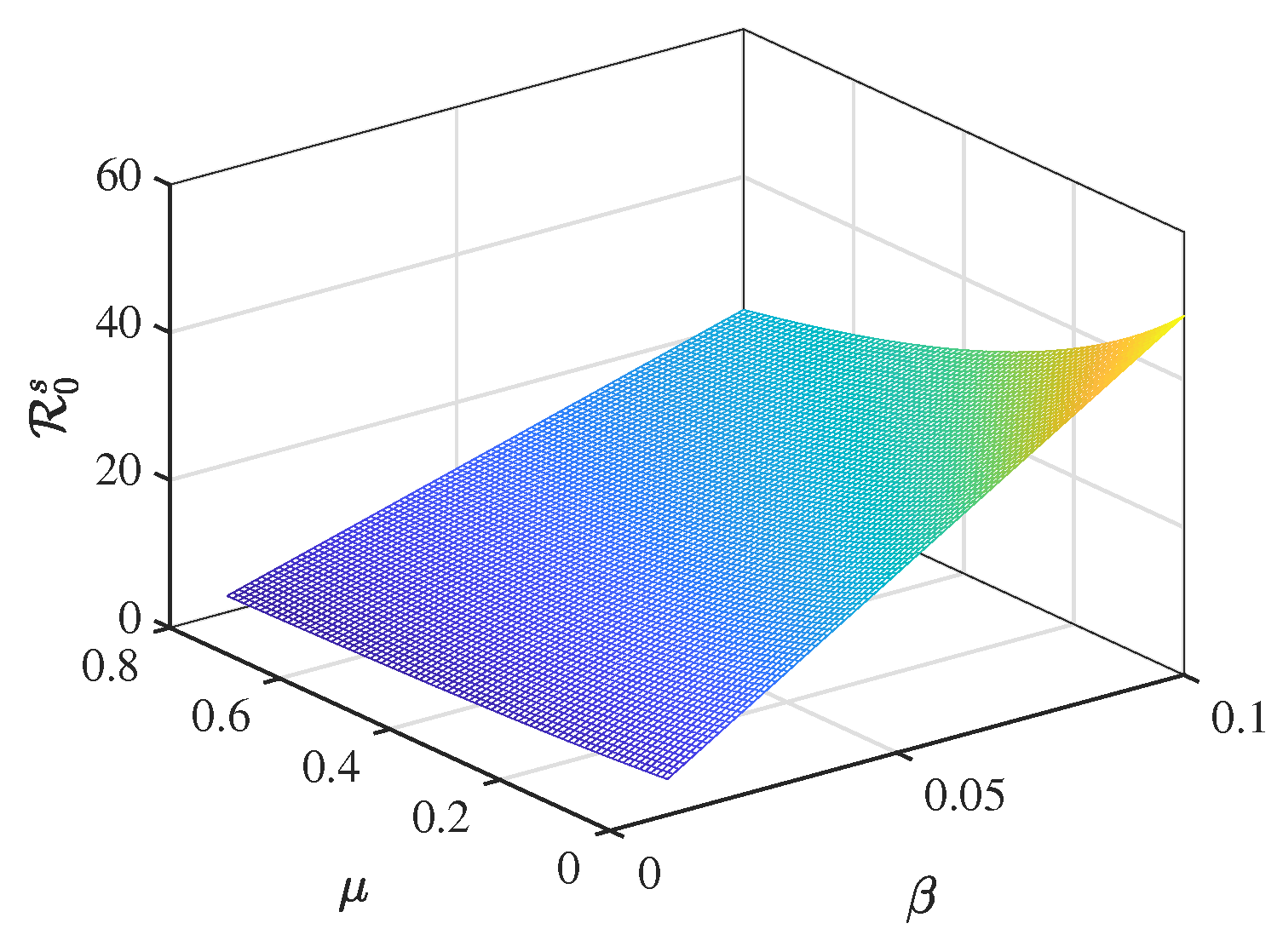
We further investigate the relationship between several parameters and the value of , as depicted in Figure 4. According to the definition of in Equation (2), it is evident that decreases as decreases or increases. To clearly illustrate the impact of and on , we fix , , , , , , and vary within the range [0.01, 0.1] and within the range [0, 0.8]. Through the analysis of Figure 4, it is evident that by reducing interpersonal contact and promoting vaccination efforts, the spread of the disease can be effectively controlled, aligning with the current strategies implemented in response to the ongoing pandemic.
5. Concluding Remarks
In this paper, we considered a stochastic SVEIR epidemic model with a nonlinear incidence rate. We utilized two key values to determine the system dynamics: one is defined as , and the other is the reproduction number of the corresponding deterministic model. We demonstrated that when , the disease will become extinct. On the other hand, if and the other parameter values satisfy the conditions in Theorem 2, the disease will persist.
We extracted feasible coefficients from published studies on COVID-19 transmission to exemplify our findings. Through our sensitivity analysis, we revealed that the stochastic model, with the introduction of random fluctuations, can effectively mitigate disease outbreaks. Specifically, the contact transmission rate and the vaccination rate coefficient exert substantial influence on the value of . These results indicate that reducing interpersonal contact and increasing vaccine usage are effective strategies for controlling epidemic spread.
The utilization of stochastic Lyapunov functions and numerical simulations with COVID-19 data accentuates the symmetrical interplay between random fluctuations, vaccination efficacy, and disease containment. This symmetrical perspective enhances our understanding of epidemic dynamics and underscores the importance of balanced strategies in mitigating disease outbreaks. As such, this study aligns with the principles of symmetry, emphasizing the harmonious interactions and equilibrium present in epidemic modeling and control efforts.
Finally, it should be noted that there are several areas that warrant further investigation in the field of stochastic epidemic modeling. For instance, (1) in the model we assumed Brownian noise, but in reality, some cases involve Lévy noise; (2) in the numerical simulation part, we assumed certain parameter values, but the actual parameter values are still uncertain; (3) the conditions outlined in Theorem 2 are intricate; (4) the nonlinear incidence rate may vary when modeling different diseases; (5) since most vaccines have a time limit, it is essential to incorporate this limitation into the model. In our future work, we will focus on addressing these questions.
Author Contributions
X.W.: conceptualization, investigation, writing—original draft. L.Z.: conceptualization, discussing, writing—review and editing. X.-B.Z.: discussing, writing—review and editing. All authors have read and agreed to the published version of the manuscript.
Funding
This work was partly supported by the Natural Science Foundation of Shaanxi Province (No. 2023-JC-YB-083), and the National Natural Science Foundation of China (Nos. 12361041, 12061033, 12201499).
Data Availability Statement
Data are contained within the article.
Conflicts of Interest
The authors declare that they have no known competing financial interests or personal relationships that could have appeared to influence the work reported in this paper.
References
- Naheed, A.; Singh, M.; Lucy, D. Numerical study of SARS epidemic model with the inclusion of diffusion in the system. Appl. Math. Comput. 2014, 229, 480–498. [Google Scholar] [CrossRef] [PubMed]
- Huo, H.F.; Feng, L.X. Global stability for an HIV/AIDS epidemic model with different latent stages and treatment. Appl. Math. Model. 2013, 37, 1480–1489. [Google Scholar] [CrossRef]
- Pongsumpun, P.; Tang, I.M. Dynamics of a new strain of the H1N1 influenza a virus incorporating the effects of repetitive contacts. Comput. Math. Methods Med. 2014, 2014, 487974. [Google Scholar] [CrossRef] [PubMed]
- Sen, M.; Ibeas, A. On an SE(Is)(Ih)AR epidemic model with combined vaccination and antiviral controls for COVID-19 pandemic. Adv. Differ. Equ. 2021, 2021, 92. [Google Scholar] [CrossRef]
- Xing, Y.; Zhang, L.; Wang, X. Modelling and stability of epidemic model with free-living pathogens growing in the environment. J. Appl. Anal. Comput. 2020, 10, 55–70. [Google Scholar] [CrossRef]
- Zhang, L.; Xing, Y.F. Stability Analysis of a Reaction-Diffusion Heroin Epidemic Model. Complexity 2020, 2020, 3781425. [Google Scholar] [CrossRef]
- Wang, X. An SIRS Epidemic Model with Vital Dynamics and a Ratio-Dependent Saturation Incidence Rate. Discret. Dyn. Nat. Soc. 2015, 2015, 720682. [Google Scholar] [CrossRef]
- Beretta, E.; Takeuchi, Y. Global stability of an SIR epidemic model with time delays. J. Math. Biol. 1995, 33, 250. [Google Scholar] [CrossRef] [PubMed]
- Ruan, S.; Wang, W. Dynamical behavior of an epidemic model with a nonlinear incidence rate. J. Differ. Equ. 2003, 188, 135–163. [Google Scholar] [CrossRef]
- Xiang, H.; Wang, Y.; Huo, H. Analysis of the binge drinking models with demographics and nonlinear infectivity on networks. J. Appl. Anal. Comput. 2018, 8, 1535–1554. [Google Scholar] [CrossRef]
- Rui, X.; Ma, Z. Global stability of a delayed SEIRS epidemic model withsaturation incidence rate. Nonlinear Dyn. 2010, 61, 229–239. [Google Scholar] [CrossRef]
- Alexander, M.; Moghadas, S. Bifurcation analysis of an SIRS epidemic model with generalized incidence. SIAM J. Appl. Math. 2005, 65, 1794–1816. [Google Scholar] [CrossRef]
- Watmough, J.; Mccluskey, C.; Gumel, A. An SVEIR model for assessing potential impact of an imperfect anti-SARS vaccine. Math. Biosci. Eng. 2006, 3, 485–512. [Google Scholar] [CrossRef] [PubMed]
- Khan, M.A.; Badshah, Q.; Islam, S.; Khan, I.; Khan, S.A. Global dynamics of SEIRS epidemic model with non-linear generalized incidences and preventive vaccination. Adv. Differ. Equ. 2015, 2015, 88. [Google Scholar] [CrossRef]
- Khan, M.A.; Khan, Y.; Khan, S.; Islam, S. Global stability and vaccination of an SEIVR epidemic model with saturated incidence rate. Int. J. Biomath. 2016, 9, 59–83. [Google Scholar] [CrossRef]
- Liu, X.; Yang, L. Stability analysis of an SEIQV epidemic model with saturated incidence rate. Nonlinear Anal. Real World Appl. 2012, 13, 2671–2679. [Google Scholar] [CrossRef]
- Yang, Y.; Zhang, C.; Jiang, X. Global stability of an SEIQV epidemic model with general incidence rate. Int. J. Biomath. 2015, 8, 1550020. [Google Scholar] [CrossRef]
- Xu, Z.; Liu, X. Backward bifurcation of an epidemic model with saturated treatment function. J. Math. Anal. Appl. 2008, 348, 433–443. [Google Scholar] [CrossRef]
- Kyrychko, Y.N.; Blyuss, K.B. Global properties of a delayed SIR model with temporary immunity and nonlinear incidence rate. Nonlinear Anal. Real World Appl. 2005, 6, 495–507. [Google Scholar] [CrossRef]
- Farrington, C.P. On vaccine efficacy and reproduction numbers. Math. Biosci. 2003, 185, 89–109. [Google Scholar] [CrossRef]
- Agaba, G.O.; Kyrychko, Y.N.; Blyuss, K.B. Dynamics of vaccination in a time-delayed epidemic model with awareness. Math. Biosci. 2017, 294, 92. [Google Scholar] [CrossRef] [PubMed]
- Gao, D.P.; Huang, N.J.; Kang, S.M.; Zhang, C. Global stability analysis of an SVEIR epidemic model with general incidence rate. Bound. Value Probl. 2018, 2018, 42. [Google Scholar] [CrossRef] [PubMed]
- Rao, F.; Mandal, P.; Kang, Y. Complicated endemics of an SIRS model with a generalized incidence under preventive vaccination and treatment controls. Appl. Math. Model. 2019, 67, 38–61. [Google Scholar] [CrossRef]
- Liu, X.; Takeuchi, Y.; Iwami, S. SVIR epidemic models with vaccination strategies. J. Theor. Biol. 2008, 253, 1–11. [Google Scholar] [CrossRef] [PubMed]
- He, Z.L.; Nie, L.F. The Effect of Pulse Vaccination and Treatment on SIR Epidemic Model with Media Impact. Discret Dyn. Nat. Soc. 2015, 2015, 3129–3132. [Google Scholar] [CrossRef]
- Zhang, T. Permanence and extinction in a nonautonomous discrete SIRVS epidemic model with vaccination. Appl. Math. Comput. 2015, 271, 716–729. [Google Scholar] [CrossRef]
- Spencer, S. Stochastic Epidemic Models for Emerging Diseases. Ph.D. Thesis, University of Nottingham, Nottingham, UK, 2008. [Google Scholar]
- Beddington, J.R.; May, R.M. Harvesting Natural Populations in a Randomly Fluctuating Environment. Science 1977, 197, 463–465. [Google Scholar] [CrossRef] [PubMed]
- Gard, T.C. Introduction to Stochastic Differential Equations; Marcel Dekker Inc.: New York, NY, USA, 1988; Volume 84, p. 19. [Google Scholar]
- Mao, X. Stochastic Differential Equations and Applications, 2nd ed.; Academic Press: Cambridge, MA, USA, 2006. [Google Scholar]
- Jiang, D.; Shi, N.; Li, X. Global stability and stochastic permanence of a non-autonomous logistic equation with random perturbation. J. Math. Anal. Appl. 2008, 340, 588–597. [Google Scholar] [CrossRef]
- Lahrouz, A.; Omari, L. Extinction and stationary distribution of a stochastic SIRS epidemic model with non-linear incidence. Stat. Probab. Lett. 2013, 83, 960–968. [Google Scholar] [CrossRef]
- Chen, C.; Kang, Y. The asymptotic behavior of a stochastic vaccination model with backward bifurcation. Appl. Math. Model. 2016, 40, 6051–6068. [Google Scholar] [CrossRef]
- Liu, Q.; Jiang, D.; Shi, N.; Hayat, T.; Alsaedi, A. Stationary distribution and extinction of a stochastic SIRS epidemic model with standard incidence. Physica A Stat. Mech. Its Appl. 2017, 469, 510–517. [Google Scholar] [CrossRef]
- Zhang, X.; Huo, H.; Xiang, H.; Meng, X. Dynamics of the deterministic and stochastic SIQS epidemic model with non-linear incidence. Appl. Math. Comput. 2014, 243, 546–558. [Google Scholar] [CrossRef]
- Liu, S.; Zhang, L.; Xing, Y. Dynamics of a stochastic heroin epidemic model. J. Comput. Appl. Math. 2019, 351, 260–269. [Google Scholar] [CrossRef]
- Zhang, L.; Liu, S.; Zhang, X. Asymptotic behavior of a stochastic virus dynamics model with intracellular delay and humoral immunity. J. Appl. Anal. Comput. 2019, 9, 1425–1442. [Google Scholar] [CrossRef]
- Cai, Y.L.; Kang, Y.; Wang, W.M. A stochastic SIRS epidemic model with nonlinear incidence rate. Appl. Math. Comput. 2017, 305, 221–240. [Google Scholar] [CrossRef]
- Allen, L. An Introduction to Stochastic Processes with Applications to Biology; CRC Press: Boca Raton, FL, USA, 2010. [Google Scholar]
- Mao, X.; Marion, G.; Renshaw, E. Environmental Brownian noise suppresses explosions in population dynamics. Stoch. Process. Their Appl. 2002, 97, 95–110. [Google Scholar] [CrossRef]
- Zhang, X.B.; Liu, R.J. The stationary distribution of a stochastic SIQS epidemic model with varying total population size. Appl. Math. Lett. 2020, 116, 106974. [Google Scholar] [CrossRef]
- Zhang, X.B.; Zhang, X.H. The threshold of a deterministic and a stochastic SIQS epidemic model with varying total population size. Appl. Math. Model. 2021, 91, 749–767. [Google Scholar] [CrossRef]
- Britton, T. Stochastic epidemic models: A survey. Math. Biosci. 2010, 225, 24–35. [Google Scholar] [CrossRef]
- Ball, F.; Neal, P. A general model for stochastic SIR epidemics with two levels of mixing. Math. Biosci. 2002, 180, 73–102. [Google Scholar] [CrossRef] [PubMed]
- Yang, Q.; Jiang, D.; Shi, N.; Ji, C. The ergodicity and extinction of stochastically perturbed SIR and SEIR epidemic models with saturated incidence. J. Math. Anal. Appl. 2017, 388, 248–271. [Google Scholar] [CrossRef]
- Khasminiskii, R.Z. Stochastic Stability of Differential Equations; Springer: Berlin/Heidelberg, Germany, 2012. [Google Scholar]
- Zhang, X.; Huo, H.; Xiang, H.; Shi, Q.; Li, D. The threshold of a stochastic SIQS epidemic model. Physica A Stat. Mech. Its Appl. 2017, 482, 362–374. [Google Scholar] [CrossRef]
- Strang, G. Linear Algebra and Its Applications; Harcourt Brace Jovanovich: Orlando, FL, USA, 1988. [Google Scholar]
- Zhu, C.; Yin, G. Asymptotic properties of hybrid diffusion systems. SIAM J. Control Optim. 2007, 46, 1155–1179. [Google Scholar] [CrossRef]
- Sinan, M.; Ali, A.; Shah, K.; Assiri, T.A.; Nofal, T.A. Stability Analysis and Optimal Control of COVID-19 Pandemic SEIQR Fractional Mathematical Model with Harmonic Mean Type Incidence Rate and Treatment. Results Phys. 2021, 22, 103873. [Google Scholar] [CrossRef] [PubMed]
- Chen, M.; Li, M.; Hao, Y.; Liu, Z.; Hu, L.; Wang, L. The introduction of population migration to SEIAR for COVID-19 epidemic modeling with an efficient intervention strategy-ScienceDirect. Inf. Fusion 2020, 64, 252–258. [Google Scholar] [CrossRef] [PubMed]
- Al Kaabi, N.; Zhang, Y.; Xia, S.; Yang, Y.; Al Qahtani, M.M.; Abdulrazzaq, N.; Nusair, M.A.; Hassany, M.; Jawad, J.S.; Abdalla, J.; et al. Effect of 2 Inactivated SARS-CoV-2 Vaccines on Symptomatic COVID-19 Infection in Adults: A Randomized Clinical Trial. JAMA 2021, 326, 35–45. [Google Scholar] [CrossRef] [PubMed]
- Wang, X.; Tang, S.; Chen, Y.; Feng, X.; Xiao, Y.; Xu, Z. When will be the resumption of work in Wuhan and its surrounding areas during COVID-19 epidemic? A data-driven network modeling analysis. Sci. Sin. Math. 2020, 50, 969–978. (In Chinese) [Google Scholar]
Figure 1.
The spread of COVID-19 when .
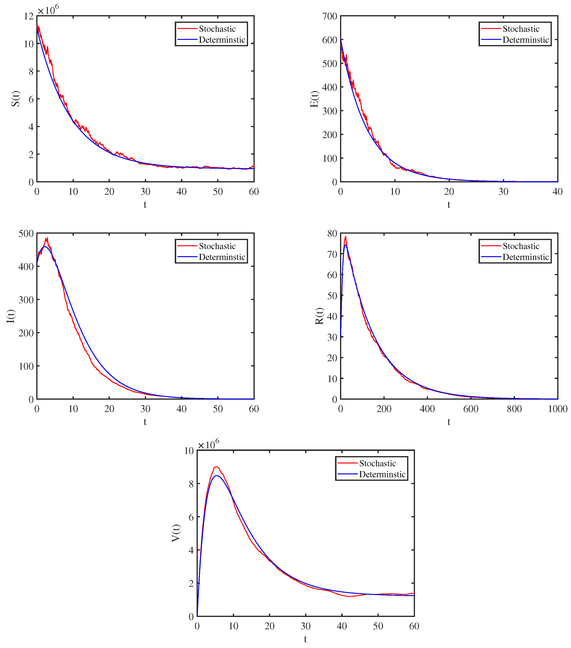
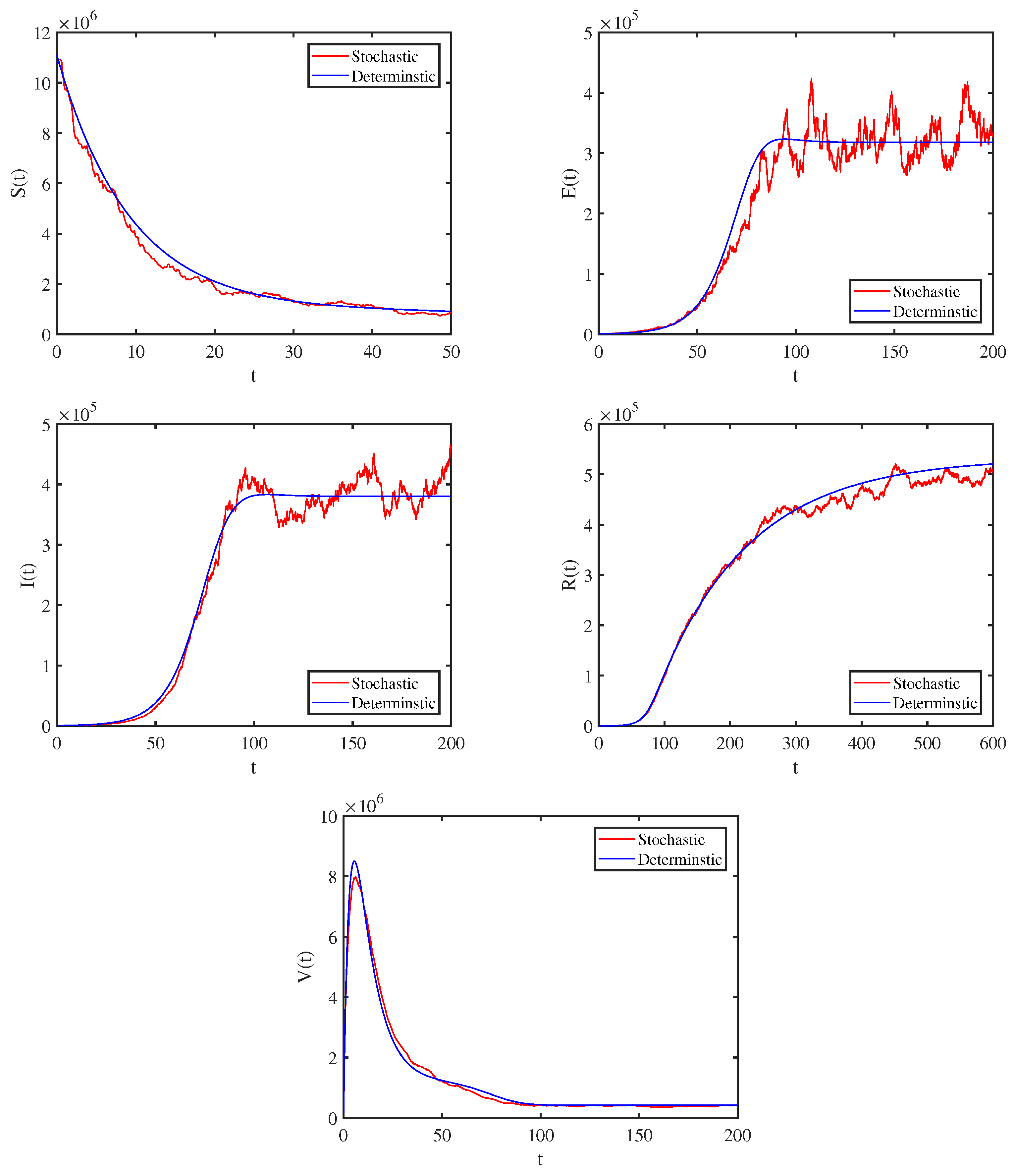
Figure 2.
The spread of COVID-19 when .

Figure 3.
The relationship between and related parameters. (a) Relationship between and . (b) Relationship between and .
Figure 3.
The relationship between and related parameters. (a) Relationship between and . (b) Relationship between and .
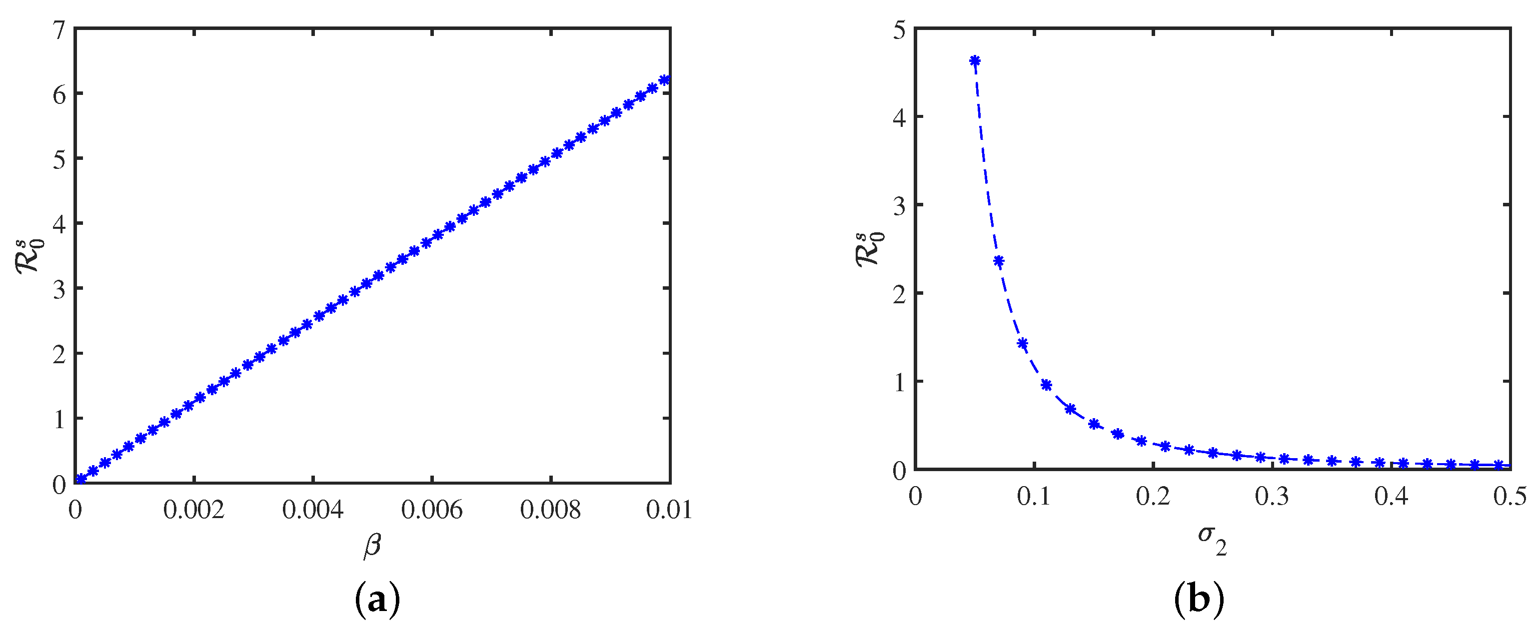
Figure 4.
Relationship between and , .


Table 1.
Biological interpretations of variables and parameters in model (1).
Table 1.
Biological interpretations of variables and parameters in model (1).
| Parameter | Description |
|---|---|
| A | The recruitment rate of new individuals |
| The contact rate or the rate of transfer of virus from an infectious individual to the susceptible | |
| The natural mortality rate | |
| The rate at which the vaccinated individuals lose their immunity and join the susceptible class | |
| The vaccination rate coefficient | |
| The rate at which exposed individuals become infectious | |
| The recovery rate of the infectious individuals | |
| The disease-related death rate of infectious individuals | |
| a | The proportion constant related to susceptible individuals |
| b | The proportion constant related to infectious individuals |
Disclaimer/Publisher’s Note: The statements, opinions and data contained in all publications are solely those of the individual author(s) and contributor(s) and not of MDPI and/or the editor(s). MDPI and/or the editor(s) disclaim responsibility for any injury to people or property resulting from any ideas, methods, instructions or products referred to in the content. |
© 2024 by the authors. Licensee MDPI, Basel, Switzerland. This article is an open access article distributed under the terms and conditions of the Creative Commons Attribution (CC BY) license (https://creativecommons.org/licenses/by/4.0/).
Share and Cite
MDPI and ACS Style
Wang, X.; Zhang, L.; Zhang, X.-B. Dynamics of a Stochastic SVEIR Epidemic Model with Nonlinear Incidence Rate. Symmetry 2024, 16, 467. https://doi.org/10.3390/sym16040467
AMA Style
Wang X, Zhang L, Zhang X-B. Dynamics of a Stochastic SVEIR Epidemic Model with Nonlinear Incidence Rate. Symmetry. 2024; 16(4):467. https://doi.org/10.3390/sym16040467
Chicago/Turabian StyleWang, Xinghao, Liang Zhang, and Xiao-Bing Zhang. 2024. "Dynamics of a Stochastic SVEIR Epidemic Model with Nonlinear Incidence Rate" Symmetry 16, no. 4: 467. https://doi.org/10.3390/sym16040467
Note that from the first issue of 2016, this journal uses article numbers instead of page numbers. See further details here.