

A 3D Descriptive Geometry Problem-Solving Methodology Using CAD and Orthographic Projection


Abstract
1. Introduction
2. Materials and Methods
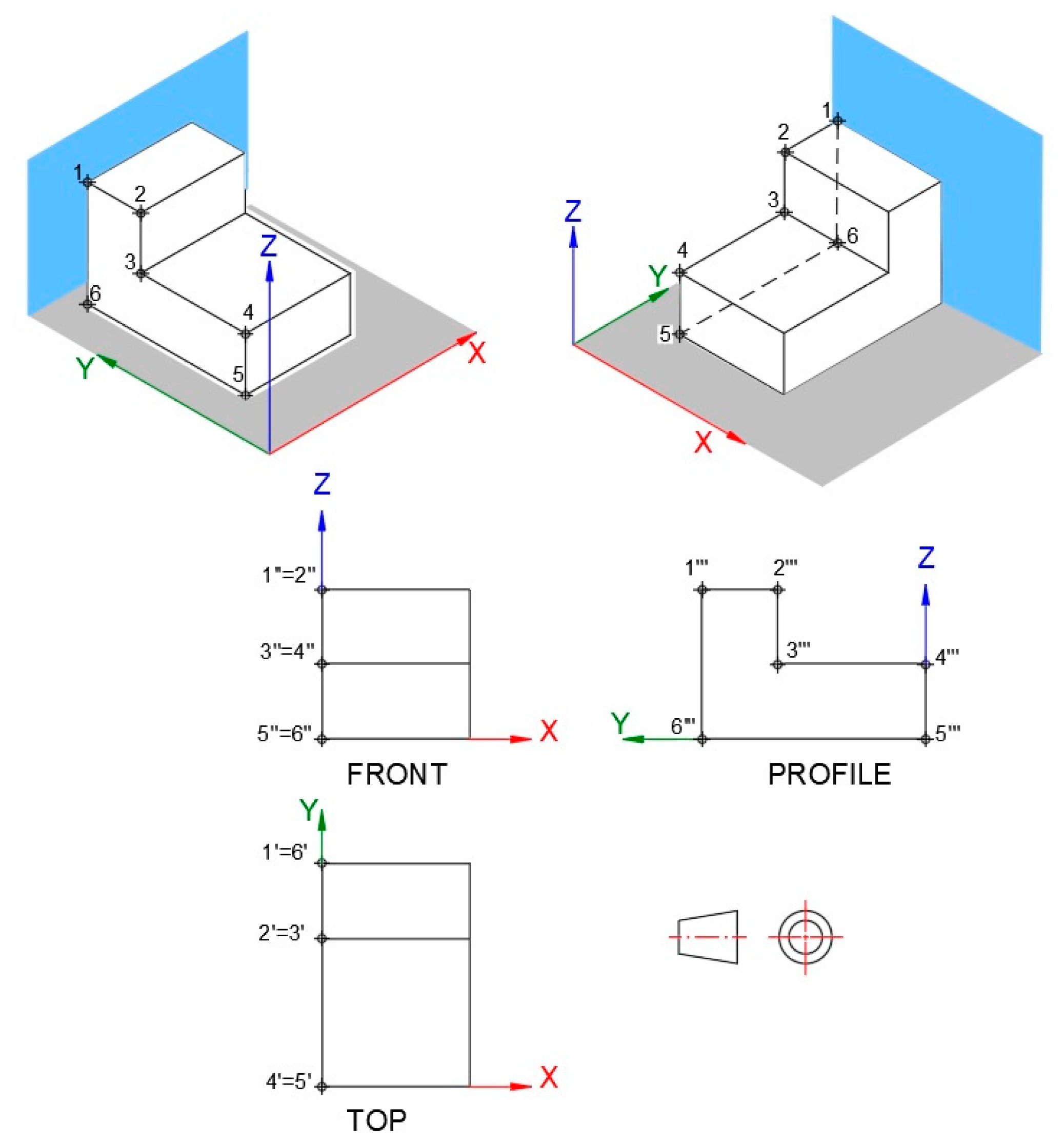
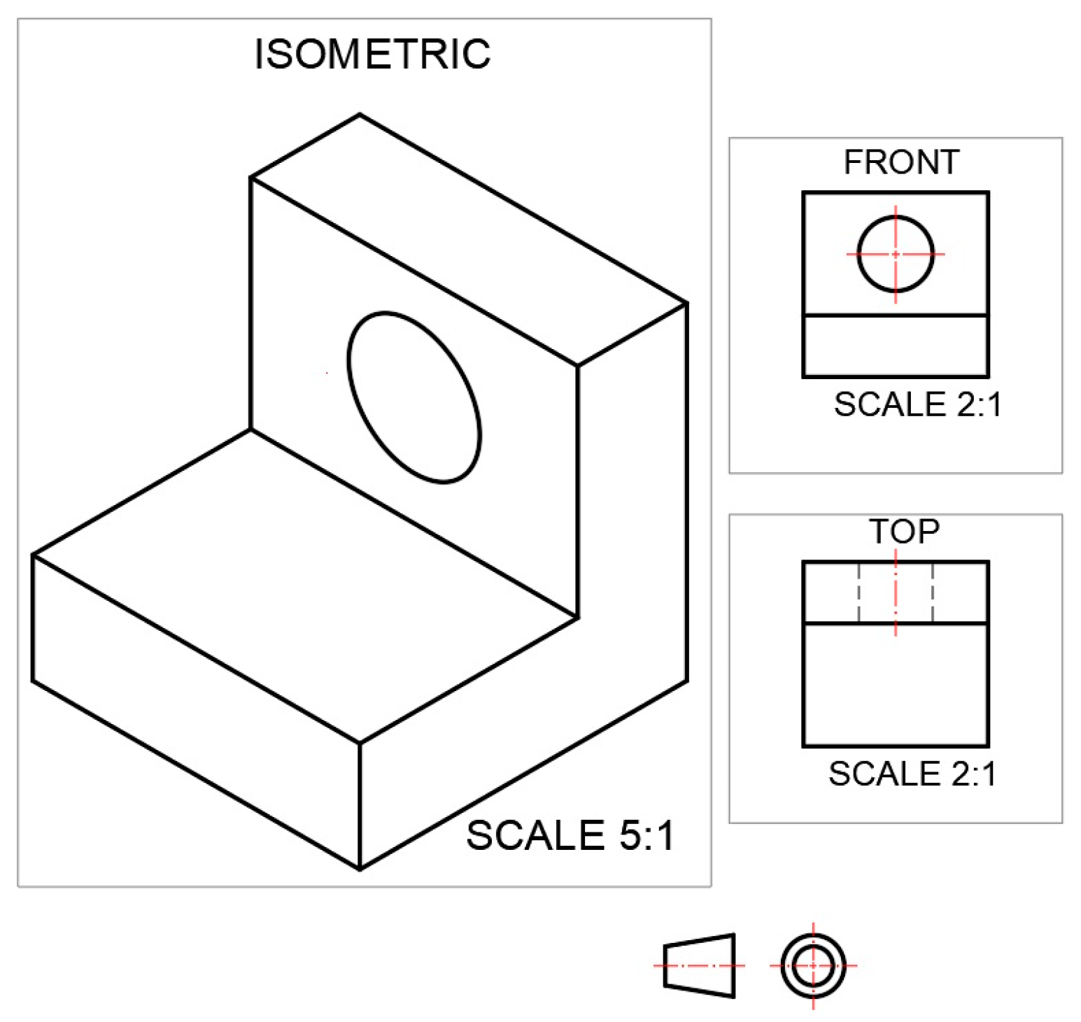
- Orthogonal views.
- Three-dimensional definition and creation of the plane main lines.
- Defining and creating views to show the true magnitude of lines and plane figures.
- Identifying, defining, and creating lines: intersecting, parallel, and perpendicular.
- Determining the angle between two coplanar lines, line and plane, and two planes.
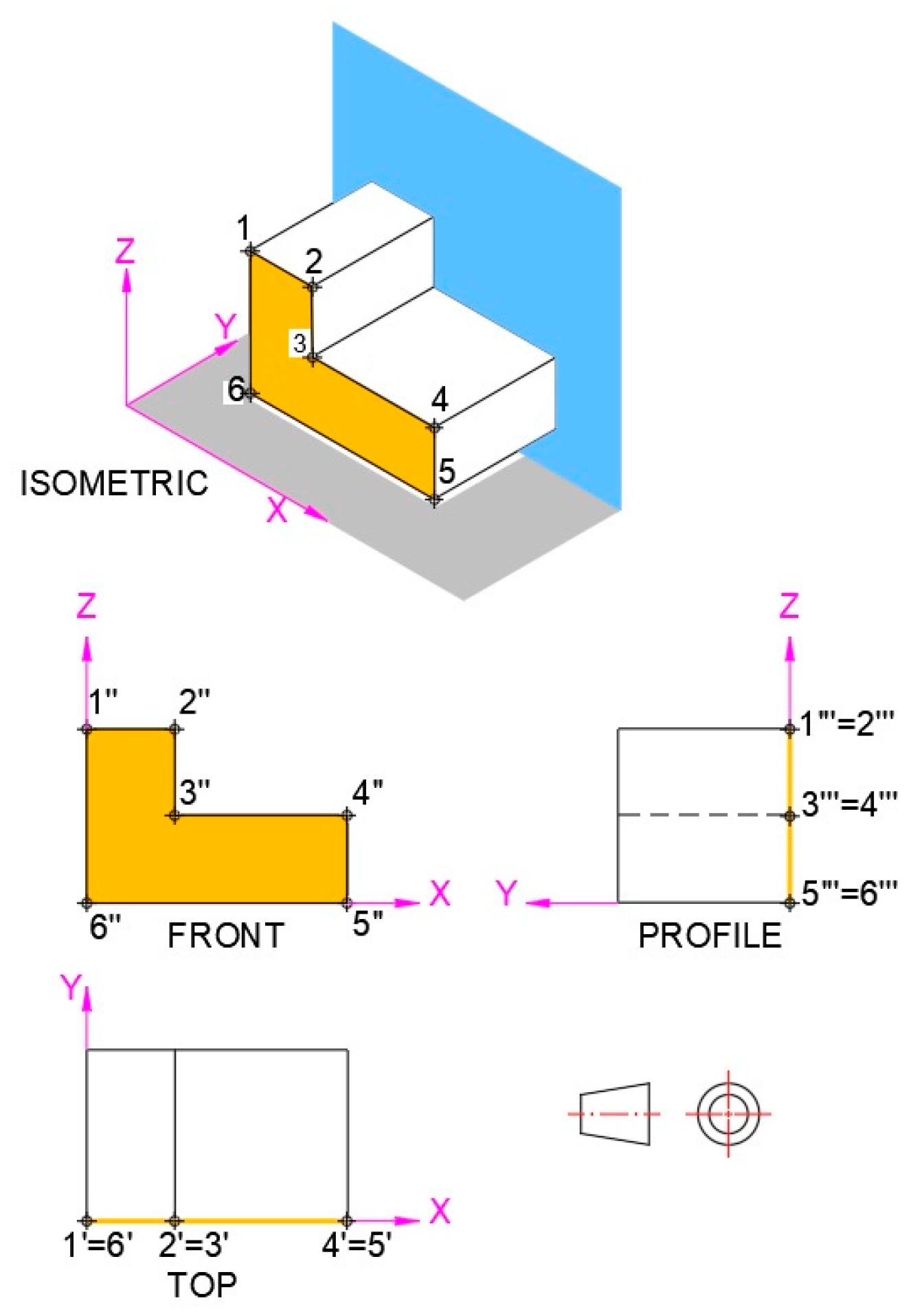
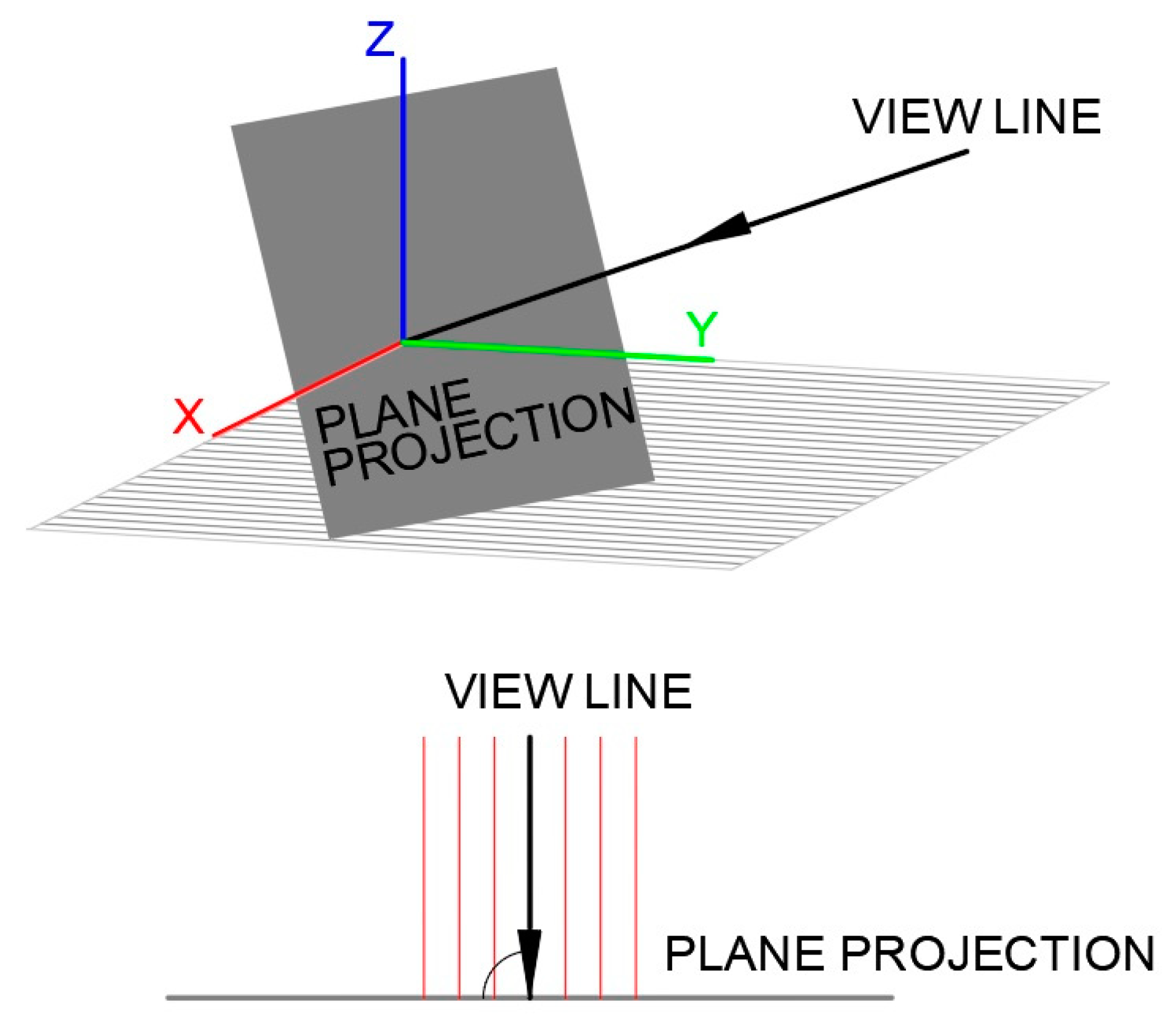
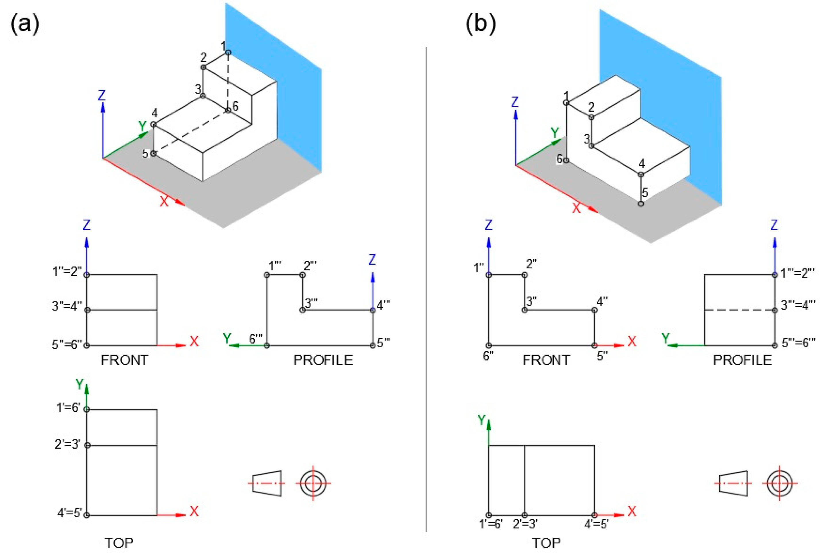
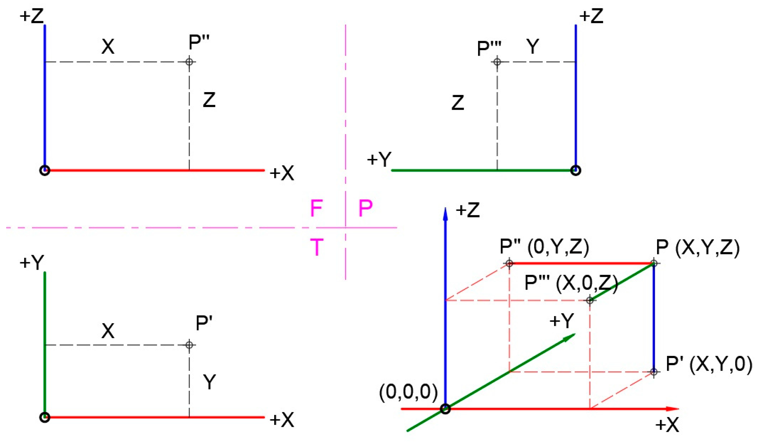
2.1. Orthographic Projection Fundamentals
2.2. CAD Fundamentals
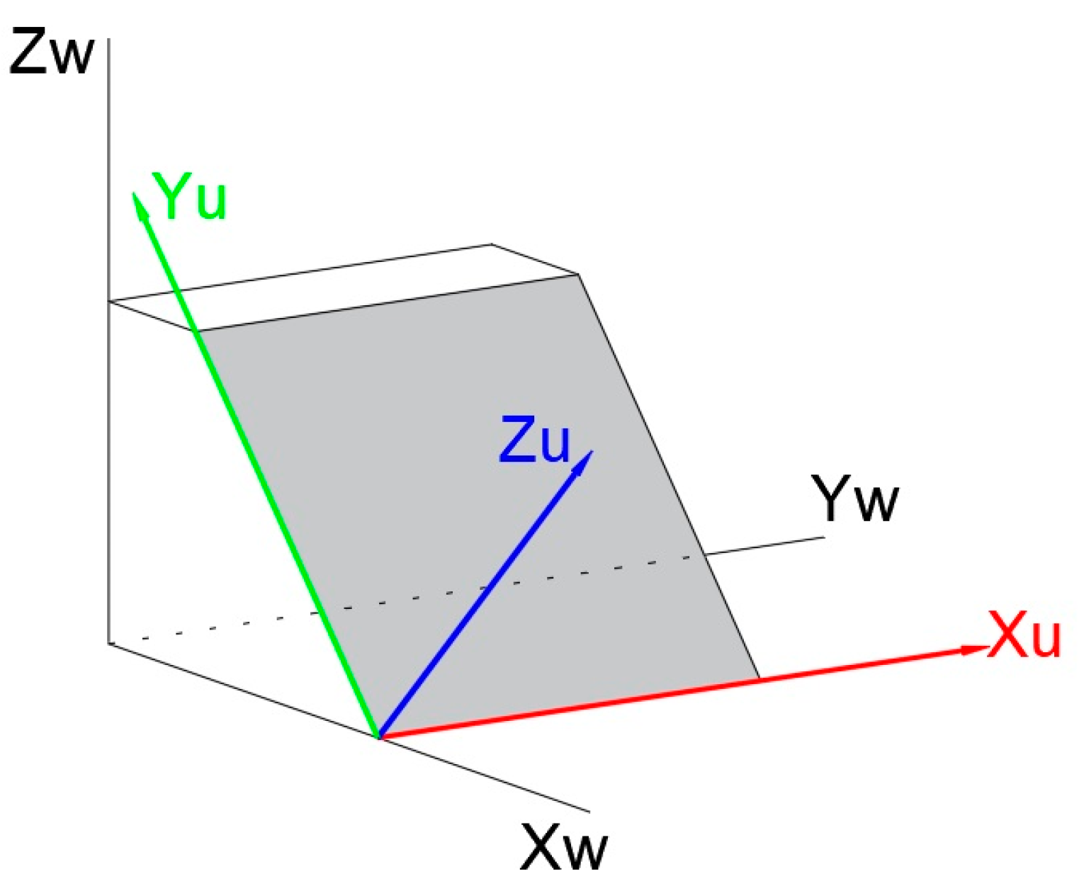
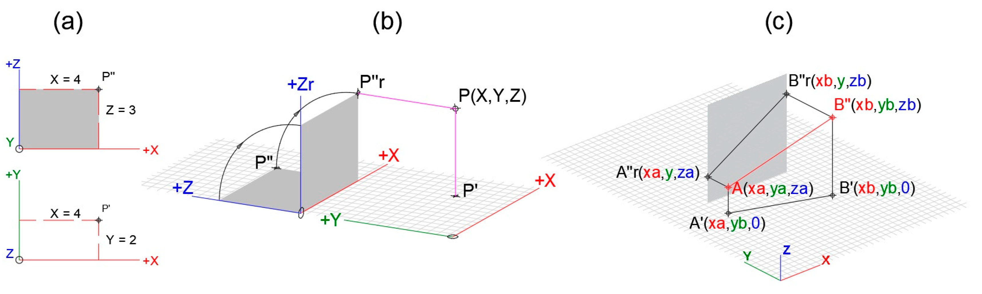
2.2.1. Reference System
- World and User Coordinate Systems
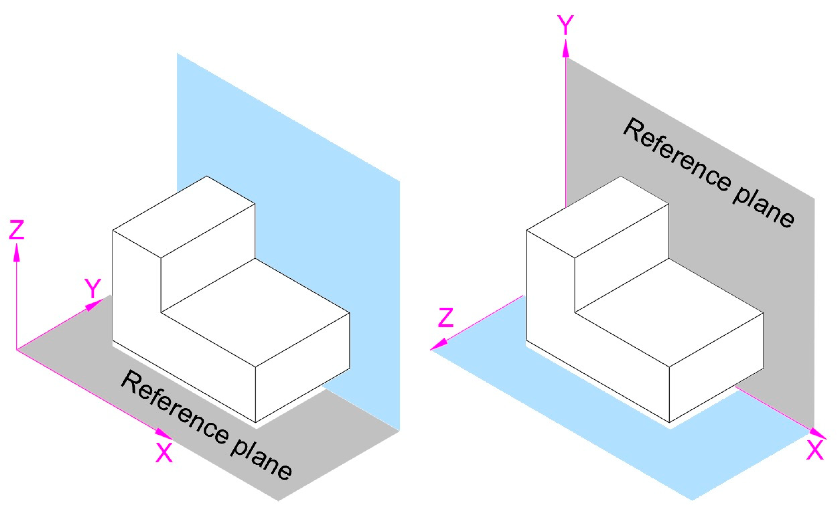
- Reference Plane
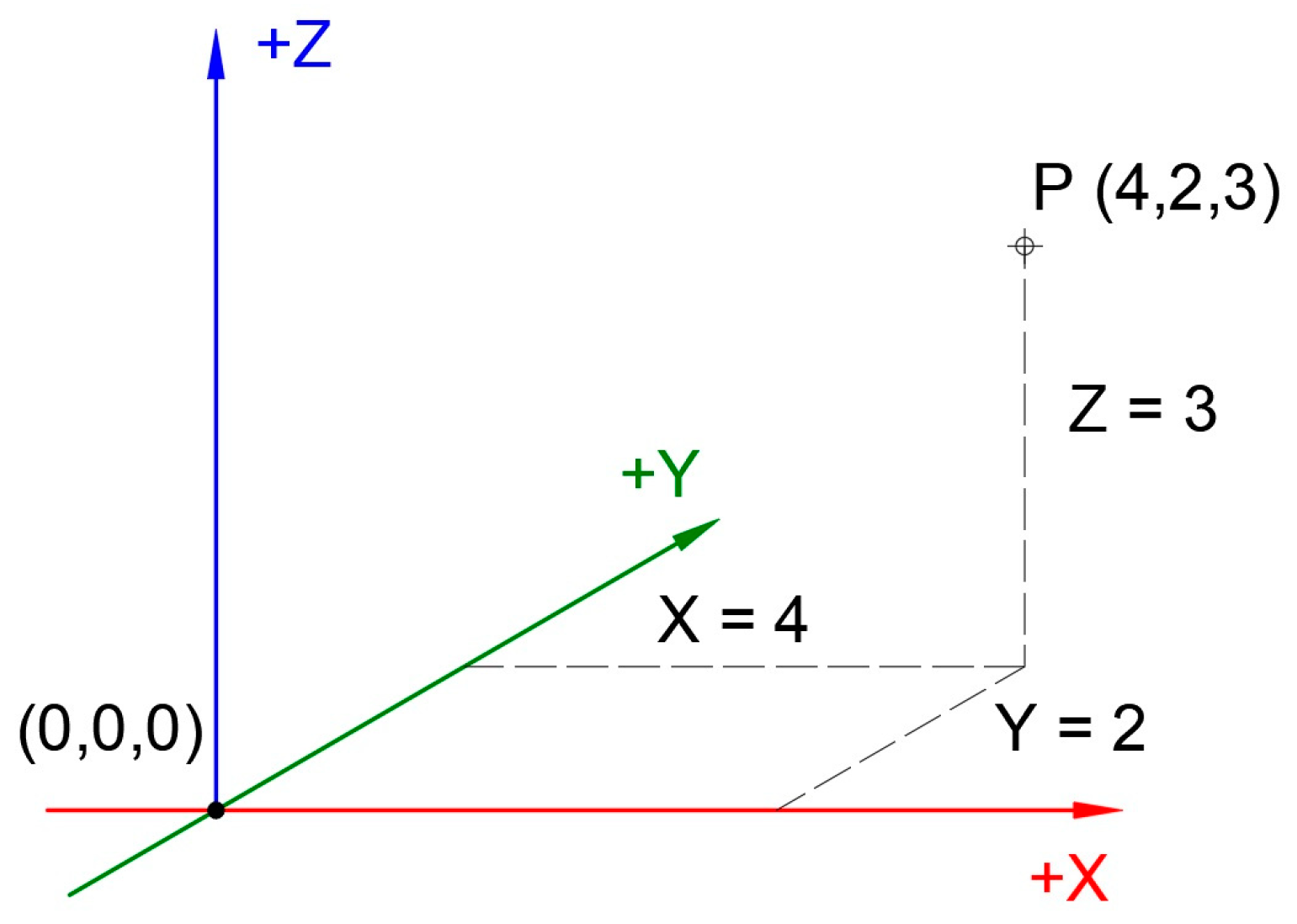
- Coordinate system
2.2.2. Viewpoint
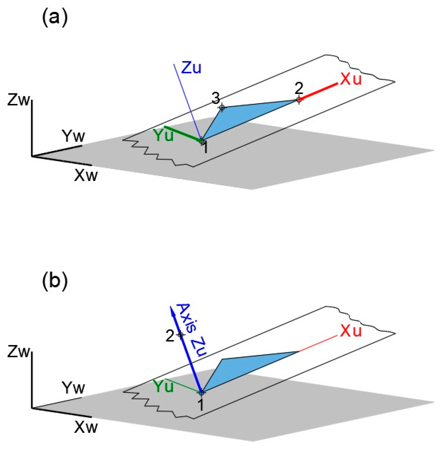
2.2.3. User Coordinate System
2.2.4. Viewports
2.3. CAD Tools
2.3.1. Rotation
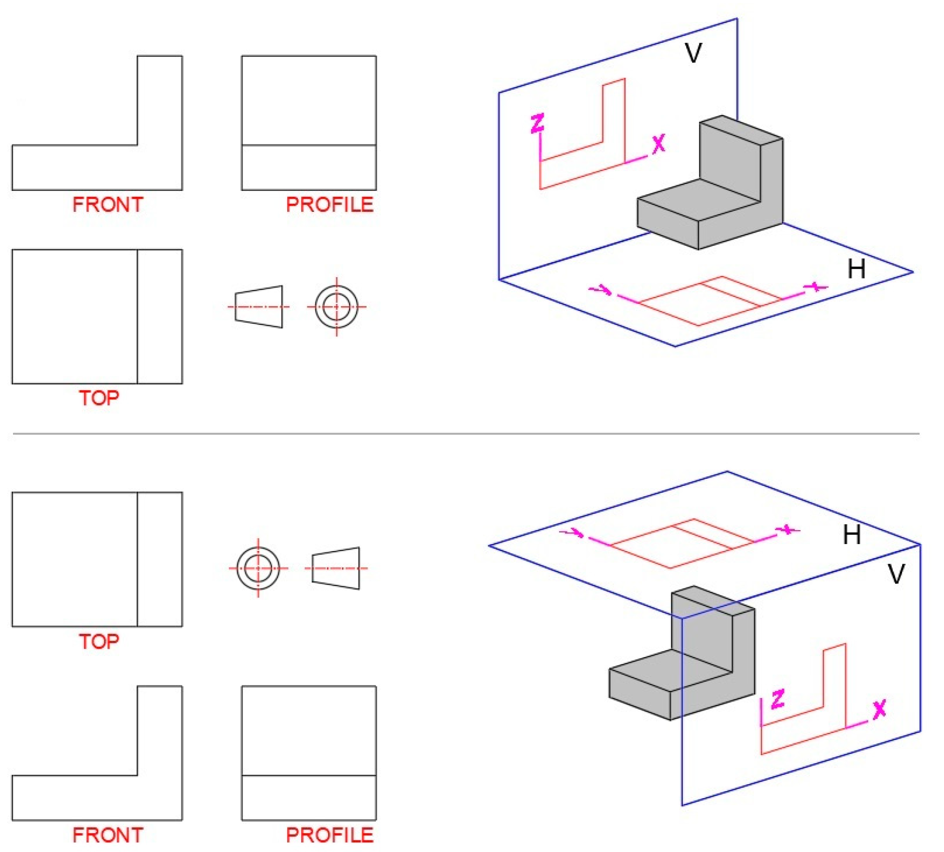
2.3.2. First-Angle and Third-Angle Projection
2.3.3. Point Filters
3. Results
3.1. Orthogonal Views
3.2. Identifying, Defining, and Creating Principal Lines of a Plane
3.3. True Length of a Line and True Size of a Plane
3.4. Parallelism and Perpendicularity
3.4.1. Parallelism between Lines
3.4.2. Parallelism between Line and Plane
3.4.3. Parallelism between Planes
3.4.4. Perpendicularity between Lines
3.4.5. Perpendicular Line from a Point to a Line
3.4.6. Perpendicular Line and Shortest Distance between Two Skew Lines
- CADOP vs. traditional method.
- CADOP solving procedure step by step.
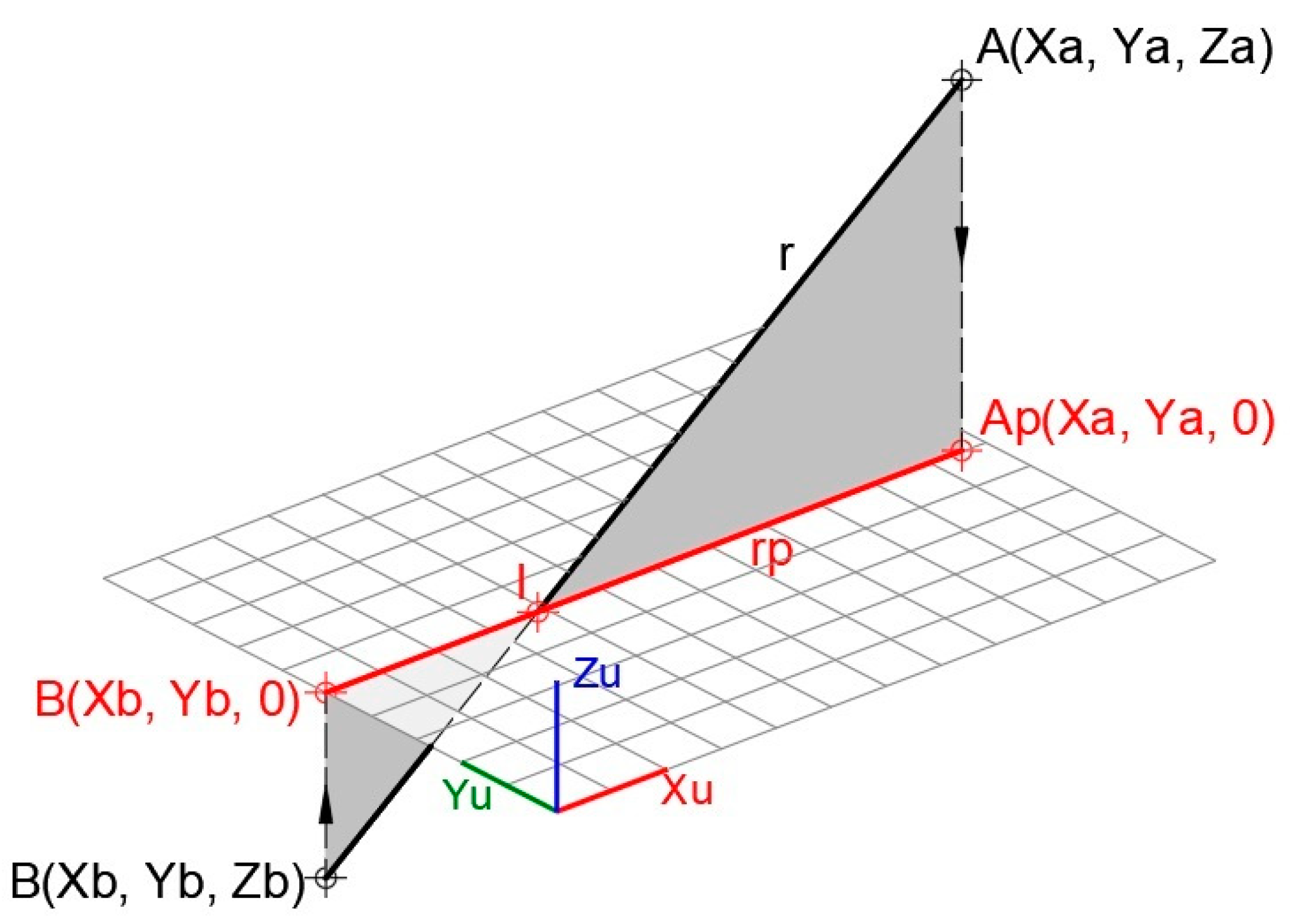
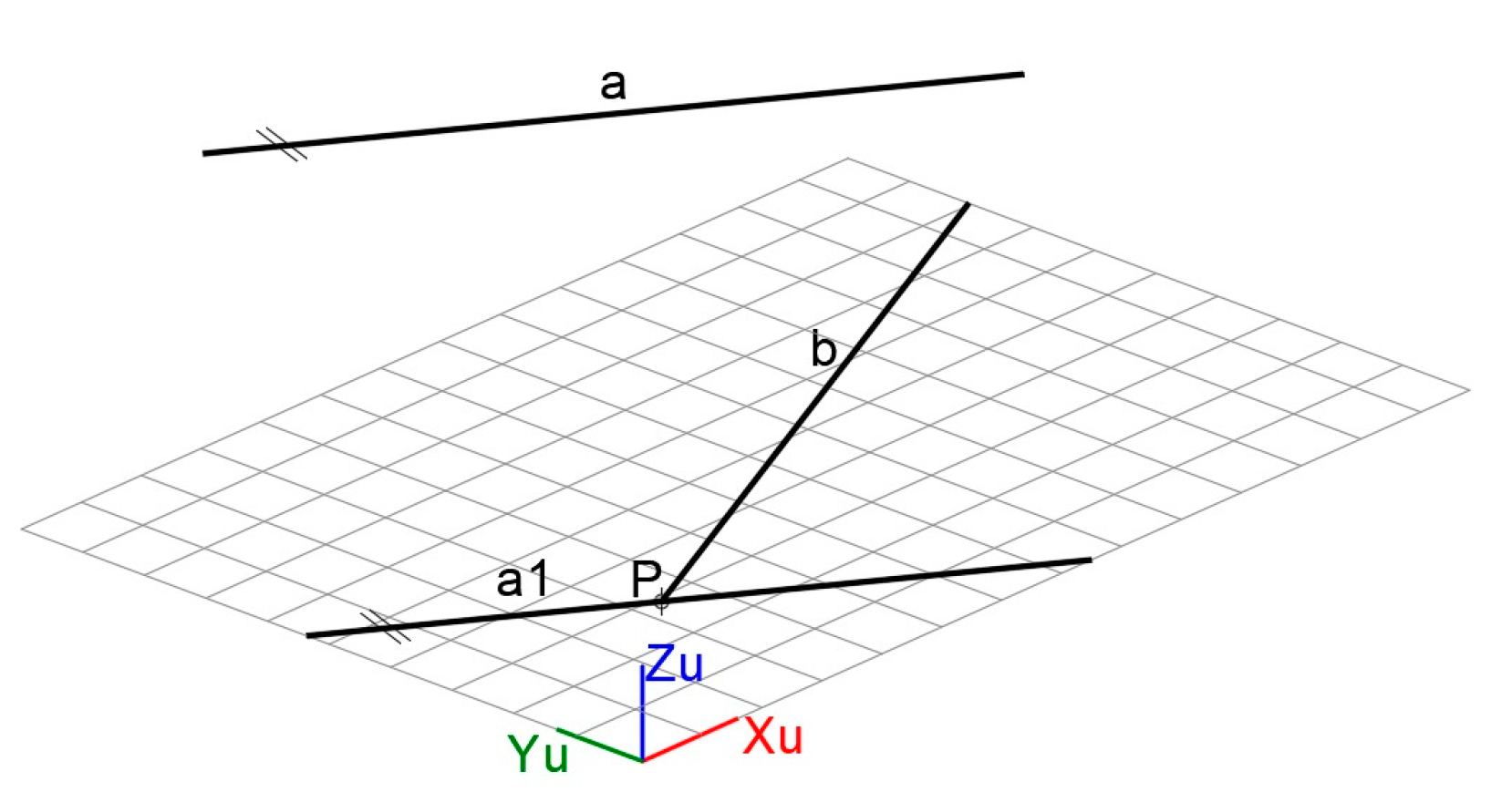
- The plane is defined through line b parallel to line a (Figure 26). Line a1 is a copy of line a through any point P on line b. The plane is determined by obtaining the UCS formed by line a1 and b.
- 2.
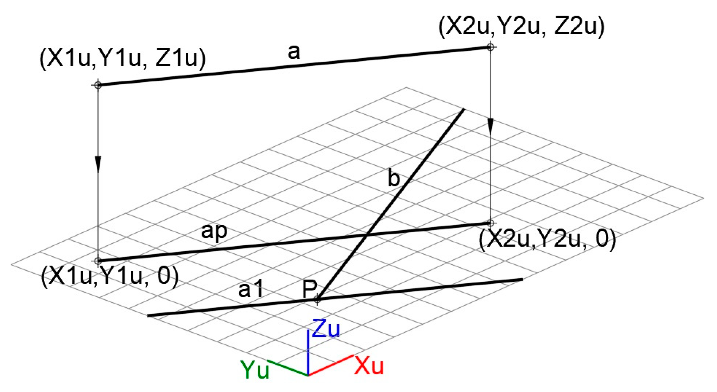
- Making Zu = 0 for any two points on line a results in a projection onto the UCS defined before. Figure 27 shows line ap resulting from the projection.
- 3.
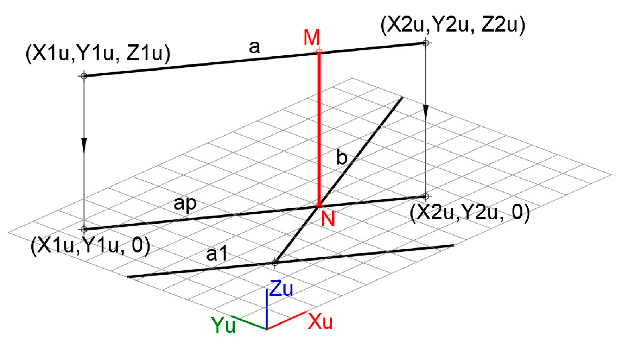
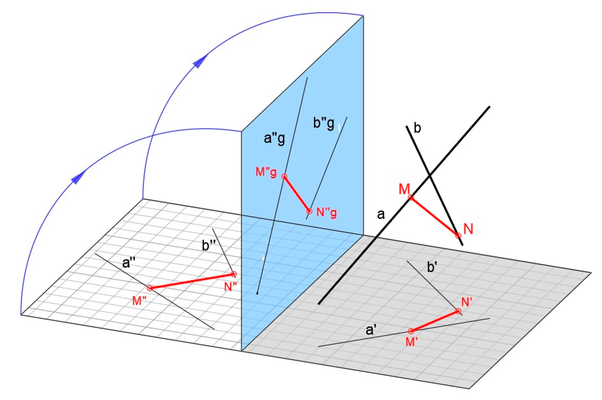
- The perpendicular line and shortest distance segment MN between lines a and b are obtained. As shown in Figure 28, the intersection of the projected line ap and line b determines point N which is one of the ends of the solution segment. The other end, point M, is the intersection of line a with the line that, drawn through N, is perpendicular to the plane defined by the UCS. Segment MN is parallel to the Z axis of this UCS, and its true length is obtained directly from the information provided by CAD.
- 4.
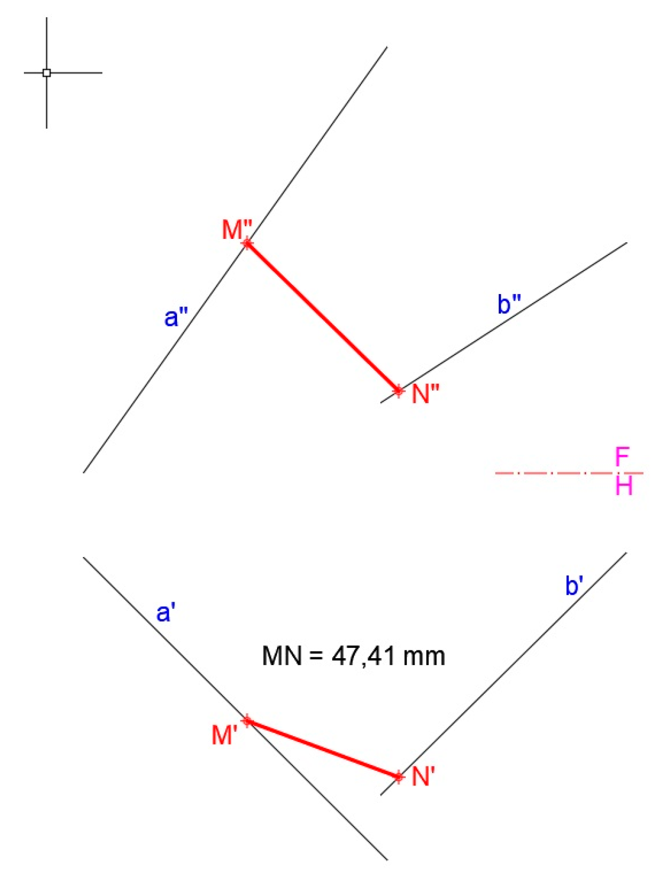
- Finally, the top and front views and true length dimension of segment MN are obtained. Figure 30 shows the solution provided by applying CADOP.
3.5. Angles
3.5.1. Angle between Two Coplanar Lines
3.5.2. Angle between Line and Plane
3.5.3. Angle between Two Planes
3.6. Regular Polyhedra
4. Conclusions
Supplementary Materials
Author Contributions
Funding
Data Availability Statement
Acknowledgments
Conflicts of Interest
References
- Bertoline, G.R.; Wiebe, E.N.; Hartman, N.W.; Ross, W.A. Technical Graphics Communications, 4th ed.; Bertoline, G.R., Ed.; McGraw-Hill Higher Education: Boston, MA, USA, 2009; pp. 691–778. ISBN 978-0-07-312837-5. [Google Scholar]
- Bokan, N.; Ljucovic, M.; Vukmirovic, S. Computer-Aided Teaching of Descriptive Geometry. J. Geom. Graph. 2009, 13, 221–229. [Google Scholar]
- Taleyarkhan, M.; Dasgupta, C.; García, J.M.; Magana, A.J. Investigating the Impact of Using a CAD Simulation Tool on Students’ Learning of Design Thinking. J. Sci. Educ. Technol. 2018, 27, 334–347. [Google Scholar] [CrossRef]
- Deng, Y.; Mueller, M.; Rogers, C.; Olechowski, A. The multi-user computer-aided design collaborative learning framework. Adv. Eng. Inform. 2022, 51, 101446. [Google Scholar] [CrossRef]
- Hunde, B.R.; Woldeyohannes, A.D. Future prospects of computer-aided design (CAD)—A review from the perspective of artificial intelligence (AI), extended reality, and 3D printing. Results Eng. 2022, 14, 100478. [Google Scholar] [CrossRef]
- Huet, A.; Pinquié, R.; Segonds, F.; Véron, P. A cognitive design assistant for context-aware computer-aided design. Procedia CIRP 2023, 119, 1029–1034. [Google Scholar] [CrossRef]
- Ramatsetse, B.; Daniyan, I.; Mpofu, K.; Makinde, O. State of the art applications of engineering graphics and design to enhance innovative product design: A systematic review. Procedia CIRP 2023, 119, 699–709. [Google Scholar] [CrossRef]
- Gradinscak, Z.B. A study on computer-based geometric modelling in engineering graphics. Comput. Netw. ISDN Syst. 1998, 30, 1915–1922. [Google Scholar] [CrossRef]
- Gradinscak, Z.B. Constructional graphics application in engineering computer graphics. J. Geom. Graph. 2001, 5, 165–179. [Google Scholar]
- Hughes, J.F.; van Dam, A.; McGuire, M.; Sklar, D.; Foley, J.; Feiner, S.; Akeley, K. Computer Graphics: Principles and Practice, 3rd ed.; Addison-Wesley: Upper Saddle River, NJ, USA, 2014; pp. 221–288. ISBN 978-0-321-39952-6. [Google Scholar]
- Boudet, J.M.F.; Talon, J.L.H. Use of Wiki as a Postgraduate Education Learning Tool: A Case Study. Int. J. Eng. Educ. 2012, 28, 1334–1340. [Google Scholar]
- Ferdiánová, V. GeoGebra Materials for LMS Moodle Focused Monge on Projection. Electron. J. E-Learn. 2017, 15, 259–268. [Google Scholar]
- Guedes, K.B.; Guimarães, M.d.S.; Méxas, J.G. Virtual Reality Using Stereoscopic Vision for Teaching/Learning of Descriptive Geometry. In eLmL 2012—Proceedings of the Fourth International Conference on Mobile, Hybrid, and On-Line Learning, Valencia, Spain, 30 January–4 February 2012; IARIA XPS Press: Wilmington, DE, USA, 2012; pp. 24–30. ISBN 978-1-61208-180-9. [Google Scholar]
- Christou, C. Virtual Reality in Education. In Affective, Interactive and Cognitive Methods for E-Learning Design: Creating an Optimal Education Experience; Tzanavari, A., Tsapatsoulis, N., Eds.; IGI Global: Hershey, PA, USA, 2010; pp. 228–243. [Google Scholar] [CrossRef]
- Chivai, C.H.; Soares, A.A.; Catarino, P. Application of GeoGebra in the Teaching of Descriptive Geometry: Sections of Solids. Mathematics 2022, 10, 3034. [Google Scholar] [CrossRef]
- Barison, M.B. Transfer of Geometric Drawing, Descriptive Geometry and Technical Drawing Classes to a Remote Model. In ICGG 2022—Proceedings of the 20th International Conference on Geometry and Graphics, São Paulo, Brazil, 15-19 August 2022; Cheng, L.-Y., Ed.; Lecture Notes on Data Engineering and Communications Technologies; Springer International Publishing: Cham, Switzerland; Boca Raton, FL, USA, 2023; Volume 146, pp. 832–842. ISBN 978-3-031-13587-3. [Google Scholar]
- Buchner, J.; Kerres, M. Media Comparison Studies Dominate Comparative Research on Augmented Reality in Education. Comput. Educ. 2023, 195, 104711. [Google Scholar] [CrossRef]
- Yaniawati, P.; Sudirman, S.; Mellawaty, M.; Indrawan, R.; Mubarika, M.P. The Potential of Mobile Augmented Reality as a Didactic and Pedagogical Source in Learning Geometry 3D. J. Technol. Sci. Educ. 2023, 13, 4–22. [Google Scholar] [CrossRef]
- Psycharis, S.; Sdravopoulou, K.; Botsari, E. Augmented Reality in STEM Education: Mapping Out the Future. In Creative Approaches to Technology-Enhanced Learning for the Workplace and Higher Education; Guralnick, D., Auer, M.E., Poce, A., Eds.; Lecture Notes in Networks and Systems; Springer Nature: Cham, Switzerland, 2023; Volume 767, pp. 677–688. ISBN 978-3-031-41636-1. [Google Scholar]
- Pasalidou, C.; Fachantidis, N.; Orfanidis, C. Utilizing Augmented Reality and Mobile Devices to Support Robotics Lessons. In Open Science in Engineering; Auer, M.E., Langmann, R., Tsiatsos, T., Eds.; Lecture Notes in Networks and Systems; Springer Nature: Cham, Switzerland, 2023; Volume 763, pp. 491–503. ISBN 978-3-031-42466-3. [Google Scholar]
- Singh, G.; Singh, G.; Tuli, N.; Mantri, A. Hyperspace AR: An Augmented Reality Application to Enhance Spatial Skills and Conceptual Knowledge of Students in Trigonometry. Multimed. Tools Appl. 2023. [Google Scholar] [CrossRef]
- Yeh, S.-H.; Qian, C.; Song, D.; Aguilar, S.D.; Burte, H.; Yasskin, P.; Ashour, Z.; Shaghaghian, Z.; Monjoree, U.; Yan, W. AR-Classroom: Augmented Reality Technology for Learning 3D Spatial Transformations and Their Matrix Representation. In Proceedings of the 2023 IEEE Frontiers in Education Conference (FIE), Madrid, Spain, 18–21 October 2023; IEEE: College Station, TX, USA, 2023; pp. 1–8. [Google Scholar]
- Anamova, R.; Dubrovin, A. About Didactic Materials Creation for the Discipline “Engineering Graphics” Based on Augmented Reality Technology. In AIP Conference Proceedings, ASEDU-II 2021—Proceedings of the II International Scientific Conference on Advances in Science, Engineering and Digital Education, Krasnoyarsk, Russian, 28 October 2021; AIP Publishing: Melville, NY, USA, 2022; Volume 2647, p. 040077. [Google Scholar] [CrossRef]
- Gutierrez de Ravé, E.G.; Jiménez-Hornero, F.J.; Ariza-Villaverde, A.B.; Taguas-Ruiz, J. DiedricAR: A Mobile Augmented Reality System Designed for the Ubiquitous Descriptive Geometry Learning. Multimed. Tools Appl. 2016, 75, 9641–9663. [Google Scholar] [CrossRef]
- Merkulova, V.A.; Tretyakova, Z.O.; Shestakova, I.G. Innovation in engineering education using AR technology on the example of disciplines “Descriptive Geometry” and “Engineering Graphics”. Perspect. Sci. Educ. 2022, 58, 243–265. [Google Scholar] [CrossRef]
- Hwang, W.-Y.; Nurtantyana, R.; Purba, S.W.D.; Hariyanti, U. Suprapto Augmented Reality with Authentic GeometryGo App to Help Geometry Learning and Assessments. IEEE Trans. Learn. Technol. 2023, 16, 769–779. [Google Scholar] [CrossRef]
- Khamrakulov, A. Organization of Effective Use of the AutoCAD Feature in Teaching Descriptive Geometry. J. Pharm. Negat. Results 2022, 13, 2644–2648. [Google Scholar] [CrossRef]


Disclaimer/Publisher’s Note: The statements, opinions and data contained in all publications are solely those of the individual author(s) and contributor(s) and not of MDPI and/or the editor(s). MDPI and/or the editor(s) disclaim responsibility for any injury to people or property resulting from any ideas, methods, instructions or products referred to in the content. |
© 2024 by the authors. Licensee MDPI, Basel, Switzerland. This article is an open access article distributed under the terms and conditions of the Creative Commons Attribution (CC BY) license (https://creativecommons.org/licenses/by/4.0/).
Share and Cite
Gutiérrez de Ravé, E.; Jiménez-Hornero, F.J. A 3D Descriptive Geometry Problem-Solving Methodology Using CAD and Orthographic Projection. Symmetry 2024, 16, 476. https://doi.org/10.3390/sym16040476
Gutiérrez de Ravé E, Jiménez-Hornero FJ. A 3D Descriptive Geometry Problem-Solving Methodology Using CAD and Orthographic Projection. Symmetry. 2024; 16(4):476. https://doi.org/10.3390/sym16040476
Chicago/Turabian StyleGutiérrez de Ravé, Eduardo, and Francisco J. Jiménez-Hornero. 2024. "A 3D Descriptive Geometry Problem-Solving Methodology Using CAD and Orthographic Projection" Symmetry 16, no. 4: 476. https://doi.org/10.3390/sym16040476
APA StyleGutiérrez de Ravé, E., & Jiménez-Hornero, F. J. (2024). A 3D Descriptive Geometry Problem-Solving Methodology Using CAD and Orthographic Projection. Symmetry, 16(4), 476. https://doi.org/10.3390/sym16040476