Abstract
There are deep historical connections between symmetry, harmonic functions, and stratified sets. In this article, we prove an analog of the removable singularity theorem for bounded harmonic functions on stratified sets. The harmonic functions are understood in the sense of the soft Laplacian. The result can become one of the main technical components for extending the well-known Poincaré–Perron’s method of proving the solvability of the Dirichlet problem for the soft Laplacian.
1. Introduction
There are deep historical connections between symmetry, harmonic functions, and stratified sets. A beautiful paper [1] by G. W. Mackey gives a systematic overview of the interplay of harmonic analysis and symmetry. At the same time, stratified sets often appear as quotients under symmetry group actions (see, for instance, [2]).
In 1926, R. Courant considered (see [3]) the oscillations of an elastic medium of a composite type: a membrane with an attached grid of strings. After a timelapse, at the end of the 1950s, M. Schechter published a series of articles that can be attributed to this subject too (see, for instance, [4]). Systematic studies in the field began at the end of the 1980s and were related to vibrations of string systems that have the form of a one-dimensional stratified set (in other words, a geometric graph, quantum graph, or topological network; see, for instance, [5]). Finally, in the 1990s, the first generalizing attempts were made to construct the theory of differential equations describing the oscillations or equilibria of intricate structures composed of elastic continua of arbitrary dimension that adjoin each other like cells in a cell complex. Such a structure is called a stratified set.
Significant progress was made in the field of elliptic second-order partial differential equations on stratified sets. The progress was achieved due to new principles for modeling such structures based on the concept of stratified measure and differential operators induced by this measure (see [6]).
The description of removable singularities for solutions of partial differential equations in a given functional space traditionally attracts significant attention from researchers. The classical result in this direction is the theorem claiming the removability of a relatively closed set of zero (harmonic) capacity for a bounded harmonic function on a domain of Euclidean space .
In this paper, we prove an analog of this theorem for bounded harmonic functions in the sense of the “soft Laplacian” on stratified sets with flat interior strata.
The main result asserts that for a bounded harmonic function on an n-dimensional stratified set satisfying the “strong sturdiness condition”, a relatively closed set is removable whenever its intersection with the closure of any n-dimensional stratum has capacity zero in that stratum.
This result can become one of the main technical components for extending the well-known Poincaré–Perron’s method of proving the solvability of the Dirichlet problem for a soft Laplacian. Previously (see [7]), this could only be done in the two-dimensional case.
This paper is further organized as follows: In Section 2, we collect preliminary information, including the definitions of a stratified set (Section 2.2); stratified measure (Section 2.2); and basic differential operators: gradient, divergence, and Laplacian (Section 2.3). In Section 2.4, we recall the mean value theorem and Harnack’s inequality for harmonic functions on stratified sets.
In Section 3, we establish our main result, namely, the removable singularity theorem, which is a straightforward consequence of Lemmas 1 and 2. The proof of Lemma 2 relies on Lemma 3, which has a rather long technical proof.
Section 4 is entirely devoted to the proof of Lemma 3. In Section 4.1, we present estimates for the gradient of a harmonic function on a stratified set (Theorem 4). These estimates generalize the corresponding results for harmonic functions in Euclidean space. In Section 4.3, we prove Theorem 5, claiming that the gradient of a harmonic function has zero flux through any admissible sphere. For harmonic functions in Euclidean space, this fact is a direct consequence of the divergence theorem, but in the setting of stratified sets, its proof becomes delicate in view of possible unboundedness of the gradient of a harmonic function near strata of dimension , where n is the dimension of the stratified set under consideration. The proof of Lemma 3 is finished in Section 4.3, and this completes the proof of the main result.
In the closing Section 5, we formulate the conclusions of the research.
2. Preliminaries
In this section we collect preliminary information concerning stratified sets, basic differential operators, and harmonic functions on stratified sets. In a more general setting, the definitions for stratified set and related notions can be found in [8,9]. To a great extent, these definitions are inspired by [10].
2.1. Stratified Sets
In this paper, by a stratified set , we mean a connected subset of the Euclidean space that consists of finitely many pairwise disjoint connected (boundaryless) submanifolds called strata. The set of all strata is denoted by , while the strata themselves are denoted by :
The first subscript indicates the dimension of a stratum, while the second enumerates the strata of the given dimension. We impose the following requirements on the mutual disposition of strata:
- The closure of every stratum is compact and the boundary is the union of some strata in ;
- For any two strata , the intersection of their closures is either empty or consists of some strata in .
Henceforth, the relation designates that . In this case, we say that the strata are contiguous (to one another).
We use the interior metric d on , where is defined as usual to be the infimum of the lengths of curves through in . It is easy to see that the metric topology agrees with the topology induced in by the inclusion . All topological notions below refer to this topology.
Also, we represent as the union (“interior” and “boundary”), in which is an open connected subset of composed of some strata in and satisfies the equality ; the remaining part is then the topological boundary of .
In this paper, all interior strata are assumed to be flat in the following sense: every stratum is a subdomain of a k-dimensional affine subspace of .
2.2. Stratified Measure
We call a set μ-measurable if every intersection is measurable with respect to the k-dimensional Lebesgue measure on . It is easy to see that the set of all -measurable sets is a -algebra on . The stratified measure on (more precisely on ) is defined as
where is the k-dimensional Lebesgue measure of the set . The measurability of a function is defined routinely: f is -measurable if all Lebesgue sets belong to for . It is easy to see that the Lebesgue integral of a -measurable function over a -measurable set reduces to the sum
We frequently omit in the notation , hoping that the stratified set under consideration is uniquely identified by the context.
2.3. Gradient, Divergence, and Laplacian
Henceforth, by , we mean the space of tangent vector fields F on whose restrictions to the strata belong to the spaces .
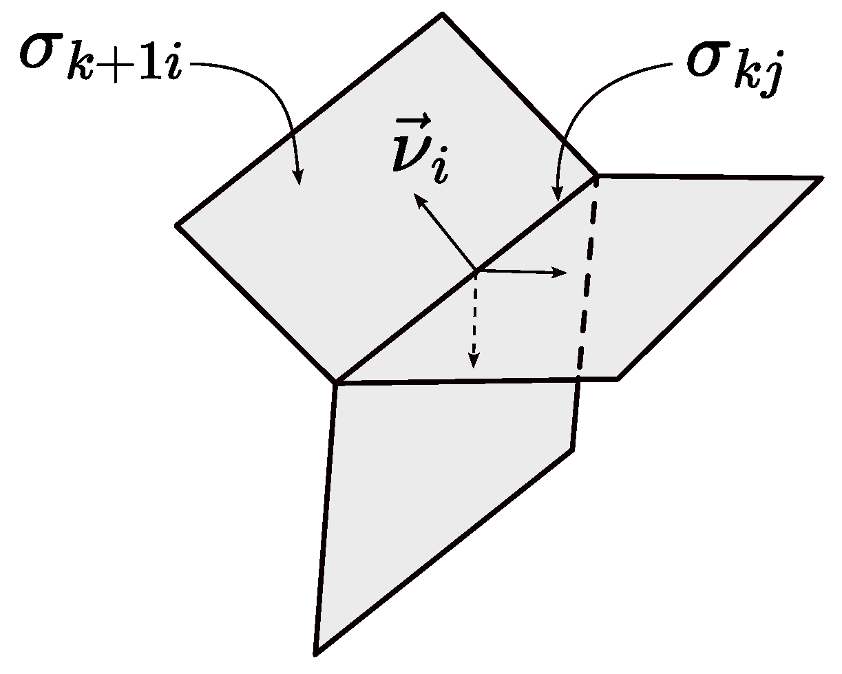
The divergence of a vector field at a point is defined to be
where the summation is carried out over all -dimensional strata contiguous to . Here, on the right-hand side denotes the operator of the conventional k-dimensional divergence applied to the restriction of to , is the unit inward normal to in at X, and is the limit of as tends to X inside in the direction of . See Figure 1 for an illustration.
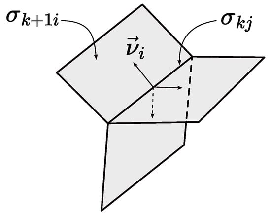
Figure 1.
Unit normals.
The so-defined divergence is a genuine analog of the classical one. It can be shown that as in the ordinary setup, the divergence is the density of the flux of the vector field at X with respect to the stratified measure defined in the previous section. Furthermore, for , we have the following stratified analog of the divergence theorem (see [6]; the sign “−” is caused by the choice of the inward normal):
where for :
with the summation taken over all not lying in .
For a sufficiently smooth scalar function u, its gradient is a tangent vector field (in this case, is simply the collection of the gradients of the restrictions of u to the strata). It would be rather natural to define the Laplacian on a stratified set as . The so-defined Laplacian is often called “hard”. At present, the qualitative theory of harmonic functions in the sense of this Laplacian is developed weakly. Therefore, here, we restrict ourselves to considering the so-called “soft” Laplacian.
We call a stratum free if it is not contiguous to any stratum of greater dimension. The soft Laplacian of a function u on is defined to be
where on the free strata and on the remaining strata.
The explicit expression of the soft Laplacian at the points of free strata coincides with the ordinary Laplacian (in the case of nonflat strata, with the Laplace–Beltrami operator).
If the stratum is not free but there exist free strata , then at a point , the expression of the soft Laplacian looks like
where the summation is taken over all free strata .
Finally, if a stratum is neither free nor contiguous to any free stratum of dimension greater by one, then, in accordance with (2), on this stratum, we have .
For an open set , we denote as the set of functions that satisfy the following conditions:
- u is continuous on U;
- For every free stratum , the restriction is twice continuously differentiable and the gradient of the restriction has a continuous extension to each point of any interior stratum contiguous to .
A function is said to be harmonic on U if and u satisfies the equation
for all .
2.4. Mean Value Theorem and Harnack’s Inequality
The functions on a stratified set that are harmonic in the sense of the soft Laplacian inherit a number of important properties of the ordinary harmonic functions. In particular, analogs of the mean value theorem and Harnack’s inequality are valid.
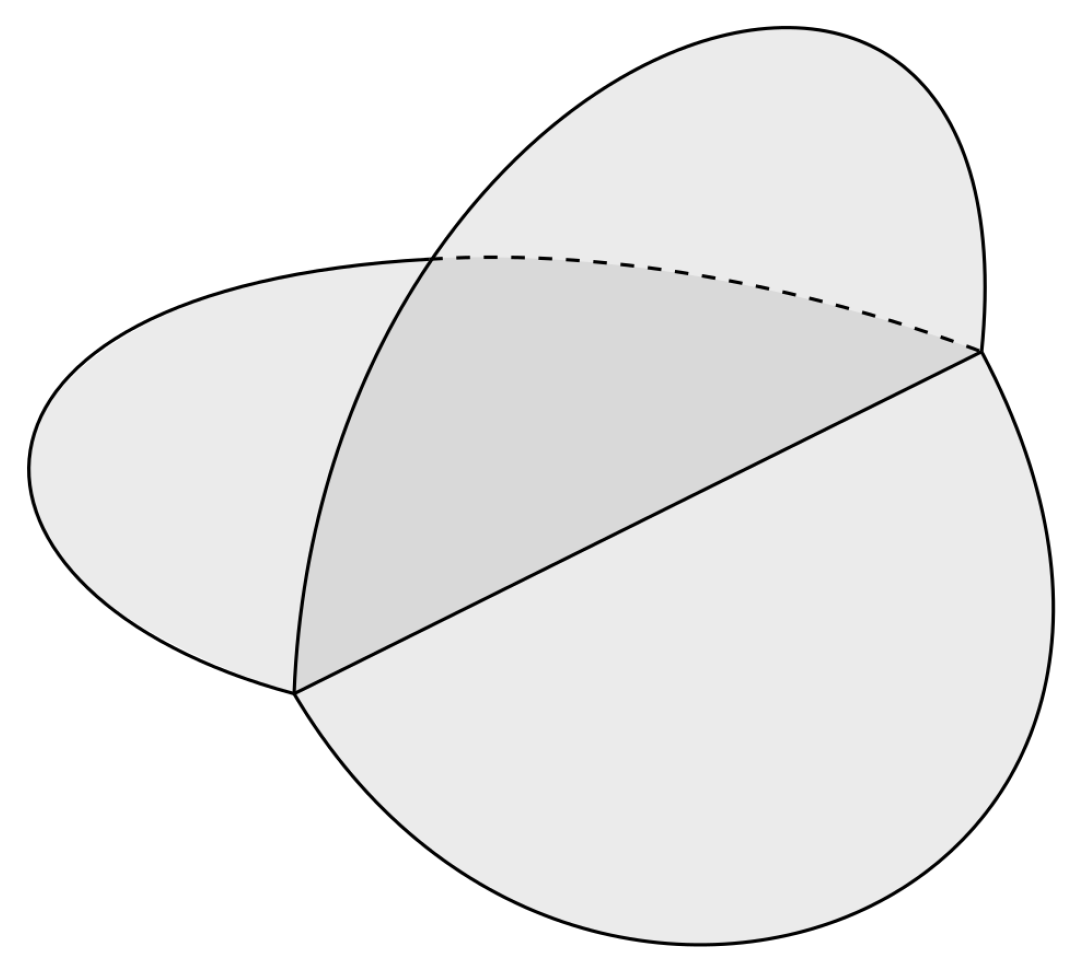
We call a ball admissible, or, in more detail, an open ball of admissible radius with center , if r is less than the distance from to any stratum whose closure does not contain . In this event, the set is called an admissible sphere. Figure 2 shows several examples of admissible balls.
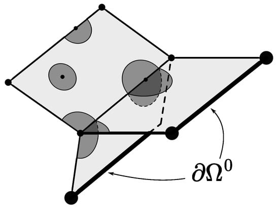
Figure 2.
Admissible balls.
Admissible balls and spheres obtain a natural stratification from . For example, for an admissible sphere S, all nonempty intersections , , are its -dimensional strata. The stratified measure on a stratified sphere S is defined as for any other stratified set (see Section 2.2).
Let be a stratified set in which all free strata have the same dimension n. Then on all n-dimensional strata and p vanishes on all other strata in .
For and an admissible sphere , consider the spherical mean:
where .
Theorem 1 ([11]).
(Mean Value Theorem) Let Ω be a stratified set whose free strata have the same dimension; let u be a harmonic function on ; and let , , be an admissible sphere. Then:
Remark 1.
A similar assertion is true with the means calculated over admissible balls in place of admissible spheres.
Theorem 2 ([12]).
(Harnack’s Inequality) Let Ω be a stratified set and let K be an arbitrary compact set in . Then, the inequality
holds for every nonnegative harmonic function u on with a constant independent of u.
3. The Main Result
In this section, we establish our main result, namely, the removable singularity theorem. It is a straightforward consequence of Lemmas 1 and 2. The proof of Lemma 2 relies on Lemma 3, which has a rather long technical proof. The proof of Lemma 3 is postponed to Section 4.
Given a stratified set , we define as the union of all interior strata of dimension k and define as the union of all interior strata of dimension at most k:
A stratified set is called sturdy (see [12]) if all free strata have the same dimension n and the set is connected. Let us call strongly sturdy if all free strata have the same dimension n and, for every , there exists an admissible ball such that the set is connected.
The following theorem is the main result of the present article.
Theorem 3 (Removable Singularity Theorem).
Let Ω be a strongly sturdy stratified set, be a relatively closed set whose intersection with the closure of any free stratum has harmonic capacity zero in the affine space including the stratum, and be a bounded harmonic function. Then, u has a harmonic extension to all of .
The theorem is a straightforward consequence of the next two lemmas.
Lemma 1.
Under the conditions of Theorem 3, the function u extends to a bounded harmonic function on .
Lemma 2.
Let Ω be a strongly sturdy stratified set of dimension n and be a bounded harmonic function. Then, u has a harmonic extension to all of .
Remark 2.
The strong sturdiness condition is essential.
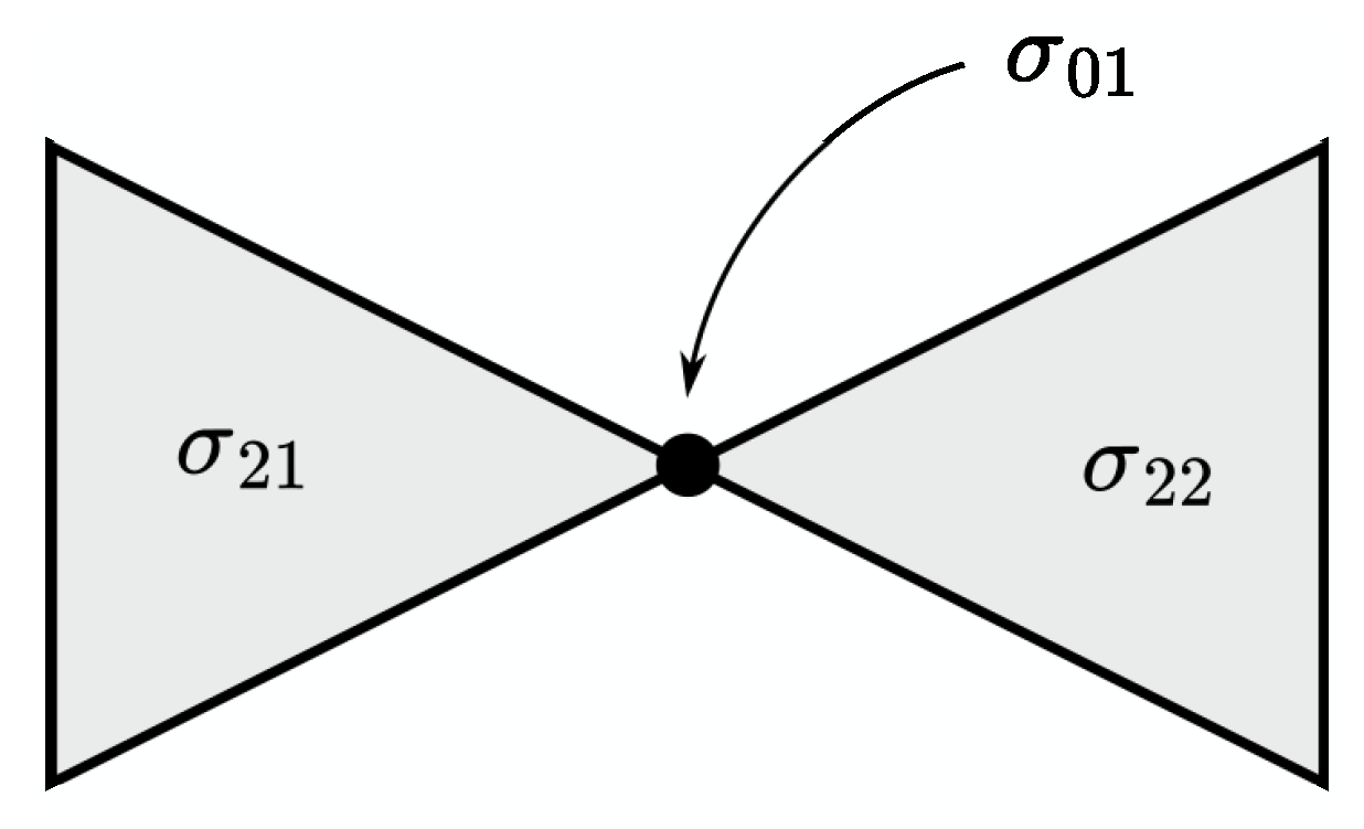
As an example, consider a two-dimensional set composed of two planar triangles with one common vertex and no other points in common (see Figure 3). Set , i.e., . The function u, which is equal to 0 on one triangle and to 1 on the other, is harmonic on , but fails to have a harmonic extension to all of .
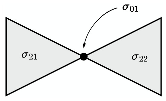
Figure 3.
Regarding Remark 2.
Proof of Lemma 1.

It suffices to prove that for every point and any admissible ball , the restriction admits an extension to a bounded harmonic function on .
If , then the existence of a sought extension follows from the removability of a relatively closed set of capacity zero for bounded harmonic functions on subdomains of . Therefore, suppose that belongs to an -dimensional stratum and let be an admissible ball. Without loss of generality, we assume to be the closed stratified ball in which serves as the interior and as the boundary (see Figure 4).
Figure 4.
Stratified ball.
Let be all strata contiguous to .
If we have exactly two strata, i.e., and , then (with its interior metric) is isometric to the usual Euclidean ball B of radius r in ; moreover, and go under isometry into half-balls separated by the -dimensional disk that is the image of . The function corresponding to u under isometry is an ordinary harmonic function on , where is the image of under isometry. Applying the standard removable singularity theorem to , we obtain a harmonic extension of to B. Executing the inverse isometry, we obtain a harmonic extension of u to .
If we have an odd number of strata, then we double their number by slightly rotating the ball around and extend u to the new strata by using this rotation.
Thus, we may assume that there are strata in total, i.e., , , that are contiguous to . Again, we take a Euclidean ball B of radius r in divided into two half-balls and resting on an equatorial -dimensional disk D. Let be an arbitrary collection of l distinct numbers and let be the complementary collection. Now, map , , onto and map , , onto isometrically so that the stratum goes onto D. Let be the union of the images of over all j under isometry. Translating u by isometry from to , we receive functions , . Proceeding similarly, we also receive functions , . It is easily seen that the function , which is equal to on and equal to on (notice that both the functions agree on the intersection of their domains), is an ordinary harmonic function on . Applying to it the standard removable singularity theorem, we obtain a harmonic extension of to the whole ball B. Since this is true for every collection J, easy combinatorics show that each individual function obtains an extension rather than their combination. Returning to u, we obtain an extension of u to the whole set for every j; furthermore, the resultant function is harmonic on the whole ball . □
Proof of Lemma 2.
Equation (3) imposes no conditions on the strata of dimension . Thus, the lemma asserts, in fact, that u extends continuously to .
We extend u from to by using spherical means. To this end, we state the following lemma whose proof is postponed to the next section.
Lemma 3 (Equality of Means).
Under the conditions of Theorem 3, for every and any admissible radii and , the equality of means holds:
Leaning on this lemma, we set
where r is any admissible radius.
Note that
Let us prove by induction on k decreasing from to 0 that is continuous on . Then, gives us the sought after extension of u.
The induction base is trivial. Suppose that is continuous on , , and hence harmonic on . Take for a k-dimensional stratum . We are to prove that
This justifies the induction step and, therefore, completes the proof of Lemma 2.
The proof of (4) is divided into Lemmas 4–6. □
Lemma 4.
Proof.
Let , , and as . Let be an admissible sphere and let be an admissible ball of a greater radius . Since the points lie on the same stratum as , the translated spheres are admissible too and lie within for large enough i. For , define
The sequence converges pointwise to u and is uniformly bounded. Therefore,
Hence,
which finishes the proof of the lemma. □
Lemma 5.
.
Proof.

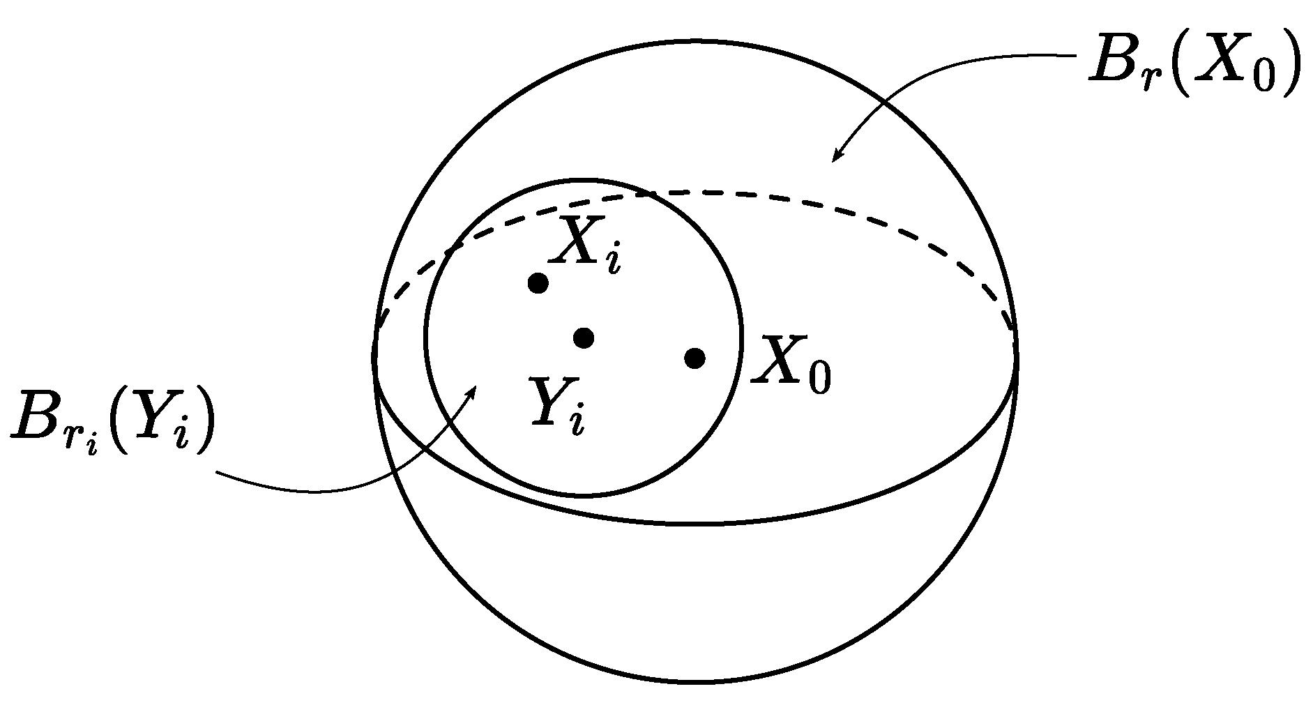
Choose so that and . Let be the k-dimensional affine plane including . Let be the projection of to . Since and , the balls , , are admissible for large enough i (see Figure 5).
Figure 5.
Regarding the proof of Lemma 5.
Since , while m is the lower limit of at , it follows that
Indeed, for any , there exists such that
Then
Notice that as . Therefore,
Inequalities (6) and (8) imply the inequality
which, by the arbitrariness of , yields
In turn, (9) and (7) imply the validity of (5).
Put
Then, are nonnegative bounded functions that are harmonic on according to the induction assumption; moreover, as .
Since all and lie on the same stratum, all (admissible) balls are similar to one admissible ball . Let denote the corresponding similarity transformation. Then,
For , define
Then, are nonnegative bounded harmonic functions on .
Let be an arbitrary compact set. Since all points are at a positive distance from the boundary of , there exists a compact set including H, as well as all the points . Taking it into account that as and applying Harnack’s inequality to the functions on and the compact set K (it is here that we use the strong sturdiness condition of ), we conclude that the functions converge uniformly to zero on K and, as a consequence, on H.
Since the compact set H can be taken arbitrarily close to and the are uniformly bounded, the means of over the spheres with center tend to zero. Indeed, let C be an upper bound for the functions and let be arbitrary. For , set
Choose so small that
Now, take the compact set
Choose N to have , , for . Then, for :
For , we obtain
Therefore, as because the spherical means of the functions and coincide in view of the equality for .
From Lemma 4, we also have . Hence, . □
Lemma 6.
.
For a proof, it suffices to apply Lemma 5 to the function , leaning upon the equality .
Lemmas 5 and 6 yield . This and Lemma 4 imply (4), thus finishing the Proof of Lemma 2.
4. Proof of Lemma 3
This section is entirely devoted to the proof of Lemma 3. In Section 4.1, we present estimates for the gradient of a harmonic function on a stratified set (Theorem 4). These estimates generalize the corresponding results for harmonic functions in Euclidean space. In Section 4.2, we prove Theorem 5, claiming that the gradient of a harmonic function has zero flux through any admissible sphere. For harmonic functions in Euclidean space, this fact is a direct consequence of the divergence theorem, but in the setting of stratified sets, its proof becomes delicate in view of possible unboundedness of the gradient of a harmonic function near strata of dimension , where n is the dimension of the stratified set under consideration. The proof of Lemma 3 is finished in Section 4.3, and this completes the proof of the main result.
4.1. Gradient Estimate
We need an estimate for the gradient of a harmonic function on a stratified set. In the classical case when u is a bounded harmonic function on a domain , we have the following gradient estimate:
where (see, for instance, [13]). We prove a similar estimate in the stratified setup.
Theorem 4 (Gradient Estimate).
Let Ω be a stratified set whose free strata have the same dimension n and let be a bounded harmonic function. Then, for every , the following estimate holds:
where is a constant depending only on the structure of the stratified set Ω and .
We first give an estimate over admissible balls.
Lemma 7.
For every and any admissible ball , the following estimate holds:
where is a constant depending only on the structure of Ω.
Proof.
We use the same trick as in the proof of Lemma 1.
If belongs to an n-dimensional stratum, then the required estimate follows from the above-mentioned classical result. We, therefore, assume that belongs to some -dimensional stratum and let be an admissible ball. Without loss of generality, we consider to be the closed stratified ball in which serves as the interior and as the boundary (Figure 4).
Let be all strata contiguous to .
If we have only two strata, namely, and , then (with its interior metric) is isometric to the ordinary Euclidean ball of radius r in ; moreover, under isometry, the strata and go onto two half-balls separated by an -dimensional disk, which is the image of . The function corresponding to u under isometry is an ordinary harmonic function on the Euclidean ball and the required estimate is valid for it. By isometry, the required estimate holds for u too.
Proceeding as in the proof of Lemma 1, we may assume that we have strata , , contiguous to . Repeating the construction from the proof of Lemma 1, we take a Euclidean ball B of radius r in divided into two half-balls and resting on an -dimensional disk D. Next, for an arbitrary collection of l distinct numbers and the complementary collection , we obtain the functions on , , and the functions on , , that correspond to the functions , , and the functions , , by isometry. Then, the function , which is equal to on and equal to on , is an ordinary harmonic function on B, and for it, we have the required estimate. Since this is true for any J, easy combinatorics show that the sought estimate is valid for each function , , and for the function u by isometry. □
Another proof can be accessed by utilizing the Poisson integral representation in admissible stratified balls centered at points of an -dimensional stratum.
The following lemma is geometrically quite evident.
Lemma 8.
If , then is an admissible radius for X. There exists (depending on Ω) such that if , then is an admissible radius for X.
Proof of Theorem 4.
Take and
If , then there is an -dimensional stratum and a point such that . Observe that . By Lemma 8, is an admissible radius for , and by Lemma 7,
If , then, by Lemma 8, is an admissible radius for X, and by Lemma 7,
Either way, we obtain the required estimate. □
4.2. Gradient Flux
Theorem 5.
Let Ω be a stratified set whose free strata have the same dimension n and let u: be a bounded harmonic function. Then, has zero flux through any admissible sphere :
Proof.

If , then the conclusion of the lemma follows from the application of the divergence theorem, which is expressed by (1), to the vector field , with the equality taken into account.
Therefore, assume . Let
be all strata whose closures contain X and dimensions do not exceed . Consider the dimensions to increase:
Note that there is exactly one stratum, namely, , of dimension , and .
Let and
Choose , , so that the sets
be pairwise disjoint for and do not intersect the strata , , that are not contiguous to .
Proceeding by induction, finally choose , , so that the sets
are pairwise disjoint for .
Set for
and consider the stratified set
with boundary
where
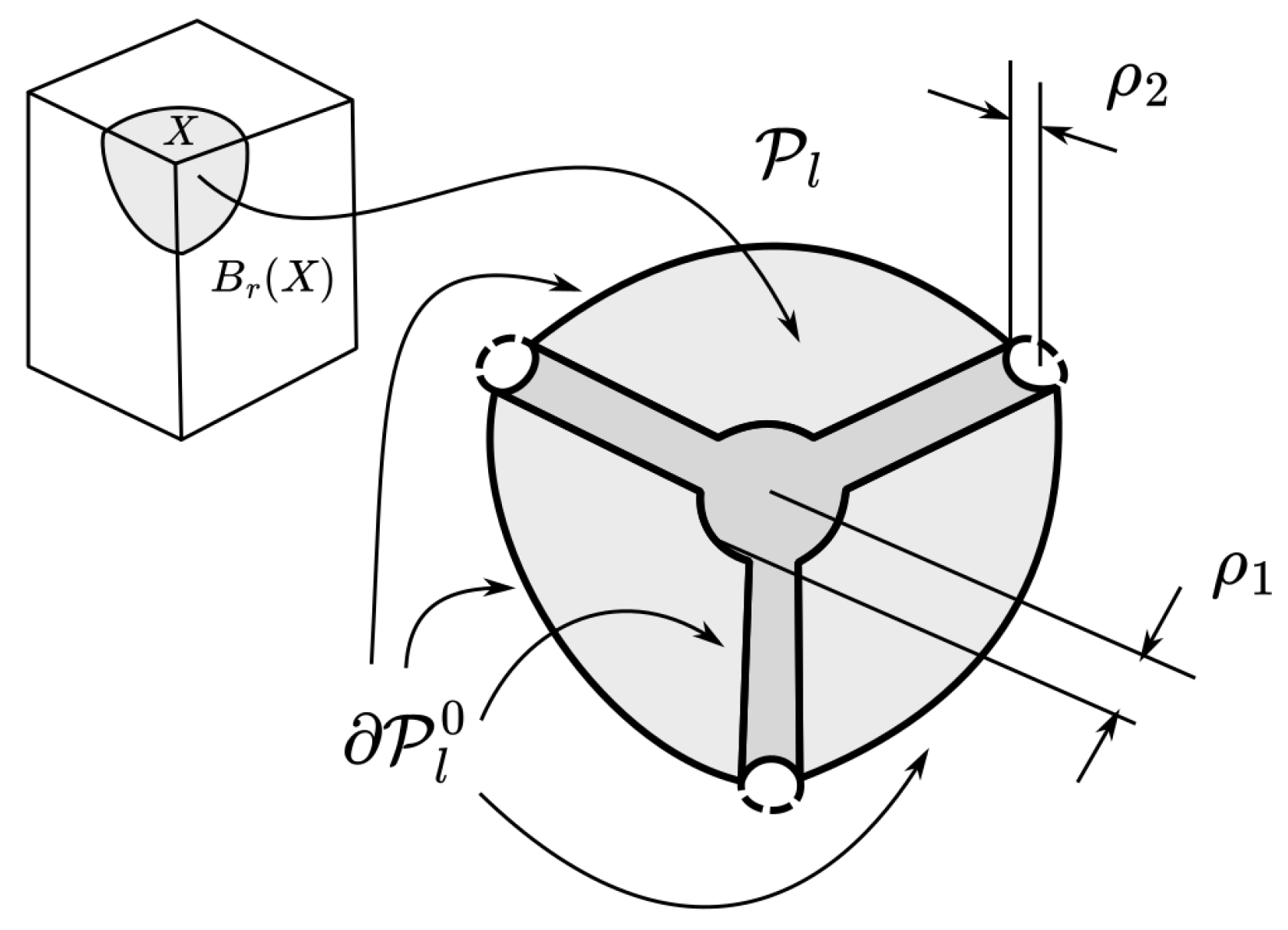
Figure 6 shows what remains after erasing the “cylinders” from the ball; in three-dimensional space, the process of constructing is not very diverse and might involve only one or two steps that depend on the dimension of the stratum containing the center of the ball. In this figure, the invisible part of the sphere is also included in the boundary .
Figure 6.
Regarding the construction of .
Inducting on l decreasing from to 0, let us prove that
where is the stratified measure on .
Take . The set represents a neighborhood of the set . Then, , and the divergence theorem (see (1)) gives
which justifies the induction base.
Assuming (11) is true, let us validate the equality for . We have
Hence,
where the signs of the integrals on the right-hand side are chosen in accordance with the fact that is part of the boundary of .
The next relations are justified below:
Applying them, we obtain the following from (12):
completing the validation of the induction step.
Since on the strata of dimension n and on the other strata, we have
where the summation is over all n-dimensional strata whose closures contain X, and is the surface -measure.
By Theorem 4, the following estimate holds:
The following lemma is rather obvious and we leave it without proof.
Lemma 9.
Let be a d-dimensional affine subspace of , , and G be an -dimensional compact piecewise smooth surface in , which is smooth in a neighborhood of the intersection and is transversal to . Then, the function
is integrable with respect to the surface -measure on G.
Note that for :
where is the affine subspace including , and is the distance from Z to inside . From (15) and (16) and Lemma 9, we then conclude that is -integrable on . This proves (13).
Fix a stratum contiguous to and consider
First, suppose that . In view of (16),
The following assertion is proven by straightforward calculations.
Lemma 10.
Let be a d-dimensional and an m-dimensional affine subspaces of , , let be a bounded open subset, and
Then,
From (19) and Lemma 10, we obtain when .
Now, we examine the case . In this case, and . To simplify the notations, we henceforth denote by , the stratum by , the stratum by , and by . Then,
and is a neighborhood of .
Let us show that the limit exists. Fix an arbitrary admissible value for and, considering , define the stratified set
whose interior and boundary are determined relative to the topology of . Note that , and by the divergence theorem:
Hence,
The last integral can be treated in the same way as in the deduction of (13). This proves the existence of the limit .
Suppose this limit is nonzero, say .
Denote by G the projection of to ,
and
If is small enough, the -measure of the difference between G and the projection of to is arbitrarily small for . In view of Theorem 4 and Lemma 10 applied with , we conclude that for sufficiently small , the values of the functions and differ by a quantity that is arbitrarily small for and, as a consequence, the following inequality holds (with some ):
Look at the integral
In the n-dimensional affine subspace including , consider the coordinates , where are the Cartesian coordinates of the projection of to the affine -dimensional subspace including , and are the polar coordinates with center in the plane orthogonal to in .
4.3. Proof of Lemma 3
Without loss of generality, we assume to have the structure of a stratified ball of admissible radius with center at a point . Consider spherical coordinates with center . Then,
For small enough , we have
where is the set of directions corresponding to the -dimensional regions of the stratified sphere . Since u is smooth on the n-dimensional strata, it follows that as :
By the finite increment formula, we have for some :
By Theorem 4:
The last inequality holds because the distance from X to increases when X moves from along a radius. Thus,
is dominated by an integrable function. By Lebesgue’s dominated convergence theorem:
The last integral vanishes in virtue of Theorem 5.
Thus,
and the value of does not depend on r, which completes the proof of Lemma 3.
5. Conclusions
The solutions of elliptic second-order partial differential equations on stratified sets inherit many properties of solutions to such equations on domains of Euclidean space. In particular, previous investigations show that analogs of the maximum priciple, the normal derivative lemma, Harnack’s inequality, etc., are valid. In this research, we established that for harmonic functions on stratified sets, an analog of the removable singularity theorem is valid as well. This result can become one of the main technical components for extending the well-known Poincaré–Perron’s method of proving the solvability of the Dirichlet problem for a soft Laplacian.
Author Contributions
Writing—original draft, N.S.D., O.M.P. and D.V.S.; Project administration, N.S.D. The authors contributed equally to this work. All authors read and agreed to the published version of the manuscript.
Funding
This research was funded by the Ministry of Science and Education of the Republic of Kazakhstan (Project AP14871251).
Data Availability Statement
The data are contained within the article.
Conflicts of Interest
The authors declare no conflicts of interest.
References
- Mackey, G.W. Harmonic analysis as the exploration of symmetry—a historical survey. Bull. Amer. Math. Soc. 1980, 3, 543–698. [Google Scholar] [CrossRef]
- Weinberger, S. The Topological Classification of Stratified Spaces (Chicago Lectures in Mathematical Series); The University of Chicago Press: Chicago, IL, USA; London, UK, 1994. [Google Scholar]
- Courant, R. Über die Anwendung der Variationsrechnung in der Theorie der Eigenschwingungen und über neue Klassen von Funktionalgleichungen. Acta Math. 1926, 49, 1–68. [Google Scholar] [CrossRef]
- Schechter, M. A Generalization of the Problem of Transmission. Ann. Della Sc. Norm. Super. Pisa 1960, 14, 207–236. [Google Scholar]
- Kuchment, P. Quantum graphs: I. Some basic structures. Waves Random Media 2004, 14, 107–128. [Google Scholar] [CrossRef]
- Pokornyi, Y.; Penkin, O.; Pryadiev, V. Differential Equations on Graphs; Fizmatlit: Moscow, Russia, 2004. [Google Scholar]
- Nicaise, S.; Penkin, O. Poincaré–Perron’s method for the Dirichlet problem on stratified sets. J. Math. Anal. Appl. 2004, 296, 504–520. [Google Scholar] [CrossRef]
- Dairbekov, N.S.; Penkin, O.M.; Sarybekova, L.O. An analog of the Sobolev inequality on a stratified set. St. Petersburg Math. J. 2019, 30, 869–875. [Google Scholar] [CrossRef]
- Dairbekov, N.S.; Penkin, O.M.; Sarybekova, L.O. The Poincaré inequality and p-connectedness of a stratified Set. Sib. Math. J. 2018, 59, 1024–1033. [Google Scholar] [CrossRef]
- Pham, F. Introduction a l’étude Topologique des Singularités de Landau; Gauthier-Villars Éditeur: Paris, France, 1967. [Google Scholar]
- Oshchepkova, S.N.; Penkin, O.M. The mean-value theorem for elliptic operators on stratified sets. Math. Notes 2007, 81, 365–372. [Google Scholar] [CrossRef]
- Dairbekov, N.S.; Penkin, O.M.; Savasteev, D.V. Harnack’s inequality for harmonic functions on stratified sets. Sib. Math. J. 2023, 64, 1137–1144. [Google Scholar] [CrossRef]
- Gilbarg, D.; Trudinger, N.S. Elliptic Partial Differential Equations of Second Order; Springer: Berlin/Heidelberg, Germany; New York, NY, USA, 2001. [Google Scholar]

Disclaimer/Publisher’s Note: The statements, opinions and data contained in all publications are solely those of the individual author(s) and contributor(s) and not of MDPI and/or the editor(s). MDPI and/or the editor(s) disclaim responsibility for any injury to people or property resulting from any ideas, methods, instructions or products referred to in the content. |
© 2024 by the authors. Licensee MDPI, Basel, Switzerland. This article is an open access article distributed under the terms and conditions of the Creative Commons Attribution (CC BY) license (https://creativecommons.org/licenses/by/4.0/).