Power Transformer On-Load Capacity-Regulating Control and Optimization Based on Load Forecasting and Hesitant Fuzzy Control

Abstract

The operational stability of a power transformer exerts an extremely important impact on the power symmetry, balance, and security of power systems. When the grid load fluctuates greatly, if the load factor of the transformer cannot be maintained within a reasonable range, it leads to increased instability in grid operation. Adjusting the transformer capacity based on load changes is of great significance. The existing control methods for on-load capacity-regulating (OLCR) transformers have low timeliness, and the daily switching frequency of the capacity-regulating switch is not controlled. To ensure the safe and stable operation of transformers, this paper proposes a control method for OLCR transformers based on load prediction and fuzzy control. Firstly, the operating principle of OLCR transformers is analyzed, and a multi-strategy enhanced dung beetle optimizer (MSDBO) combined with a CNN−LSTM model is proposed for load forecasting. On this basis, the daily switching frequency of the capacity-regulating transformer is introduced, and hesitant fuzzy control is used to select the optimal capacity-regulating strategy relying on three factors: loss, economy, and switching frequency. Finally, simulation models are constructed using the MATLAB/SIMULINK platform and simulation analysis is conducted to verify the effectiveness and superiority of the proposed control method. For the three scenarios in this paper, the method reduces daily power loss by 28.5% to 56.3% and daily operating costs by 25.4% to 50.8%. The method used in this paper can sacrifice 3.5% to 9.2% of the loss reduction capability in exchange for reducing the number of switch operations by 28.6% to 57.1%, significantly extending the lifespan of the switches and thereby increasing the operational lifespan of the transformer.

1. Introduction

Power transformers play a crucial role in ensuring the three-phase symmetry and stability of power transmission in the power system [1]. Serving as the infrastructure for power transmission and distribution, transformers are widely used in industries, agriculture, transportation, and other fields [2]. With the development of various sectors, the scale of power generation and consumption is continuously expanding, leading to a gradual increase in the capacity and voltage levels of power transformers [3]. As the scale of transformers expands, their ability to operate stably has become one of the key factors determining whether the power system can maintain symmetry and balance [4,5].

Excessive or insufficient load on transformers can present a potential hazard to the functioning of the electrical grid [6]. Prolonged operation of transformers under overload conditions may result in significant temperature rises and even lead to safety incidents, such as damage [7,8]. On the other hand, extended periods of light or no load can cause substantial power losses and economic damage [9,10]. Therefore, it is of paramount importance to judiciously adjust the rated capacity of transformers in engineering applications based on actual circumstances.

The use of on-load capacity-regulating transformers has proven to be effective in addressing the above issues. On-load capacity-regulating (OLCR) transformers are divided into two modes: high capacity and low capacity. When the grid load is high, exceeding the transformer’s critical load, the transformer adjusts to the high-capacity mode, effectively avoiding overload issues. Conversely, when the grid load is low, below the transformer’s critical load, the transformer switches to the low-capacity mode, effectively preventing significant power losses in light or no-load conditions [11,12].

Scholars from both domestic and international backgrounds have extensively researched the topic of the control of OLCR transformers. This includes analyses of the principles behind OLCR transformers, the selection of OLCR schemes, and the application of neural network methods to the control of on-load capacity regulation.

Reference [13] has demonstrated the feasibility of two methods for capacity regulation: no-load capacity regulation with automatic voltage regulation and on-load capacity regulation. Reference [14] conducts an analysis of the structural characteristics of OLCR transformers, elucidating the principles behind capacity regulation. Additionally, it provides OLCR schemes for such transformers from an economic perspective. In reference [15], a capacity regulation scheme for on-load transformers with composite switches is proposed. The study demonstrates that the parallel connection of buffering resistors at both ends of the capacity-regulating switch can effectively suppress overcurrent and overvoltage generated during capacity regulating. Based on the principles of capacity-regulating transformers, reference [16] conducts an analysis of the changes in losses, magnetic flux density, and impedance before and after capacity regulating in on-load capacity-regulating transformers. The study proposes a method for calculating the optimal capacity-regulating selection node. Reference [17] explores and designs strategies for the economic and safe operation of on-load capacity-regulating transformers. Reference [18] provides a method for calculating critical economic capacity. The study includes the design of a control system for no-load capacity-regulating transformers and proposes a switching strategy based on a gray theory load forecasting model. The above methods focus on selecting the optimal capacity-regulating node based on the economic considerations of the transformer but do not address the control of the daily switch operation frequency. In response to the issue of the irrational setting of the optimal capacity-regulating node, reference [19] proposes a method for selecting the optimal capacity-tap node for OLCR transformers based on fuzzy control. Reference [20] introduces an improved model that combines the fuzzy consistent matrix control method with the fuzzy preference method. This model applies fuzzy matrix conversion relationships to determine the weights of various indicators. Comparative analysis of the comprehensive evaluation results for a case with the analytic hierarchy process, evidence theory, and super-efficiency data envelopment analysis further demonstrates the applicability and credibility of this evaluation method. Reference [21] introduces a control strategy for on-load capacity-regulating transformers based on load forecasting. The effectiveness of this strategy is validated through experimentation. The mentioned studies primarily focus on transformer power losses and economic factors. They achieve capacity-regulating control by periodically monitoring actual values or using load forecasting. However, there is a lack of comprehensive consideration for factors such as transformer power losses, economic aspects, and the daily frequency of capacity-regulating switch operations.

This paper proposes a power transformer OLCR control and optimization method based on both load forecasting and fuzzy control, which comprehensively consider power losses, economic aspects, and the daily switching frequency all together. To address the issue of insufficient capacity switching for power transformers during frequent grid fluctuations, a method using load forecasting is proposed. This method involves training neural network models on the daily load data of transformers to construct a load forecasting model that enables real-time load prediction and capacity regulation of transformers. Furthermore, hesitant fuzzy control is employed to optimize the capacity-regulating scheme. This approach aims to proactively understand and perceive transformer loads, ultimately achieving rapid and accurate regulation of transformer capacity. The main contributions of this paper are summarized as follows:

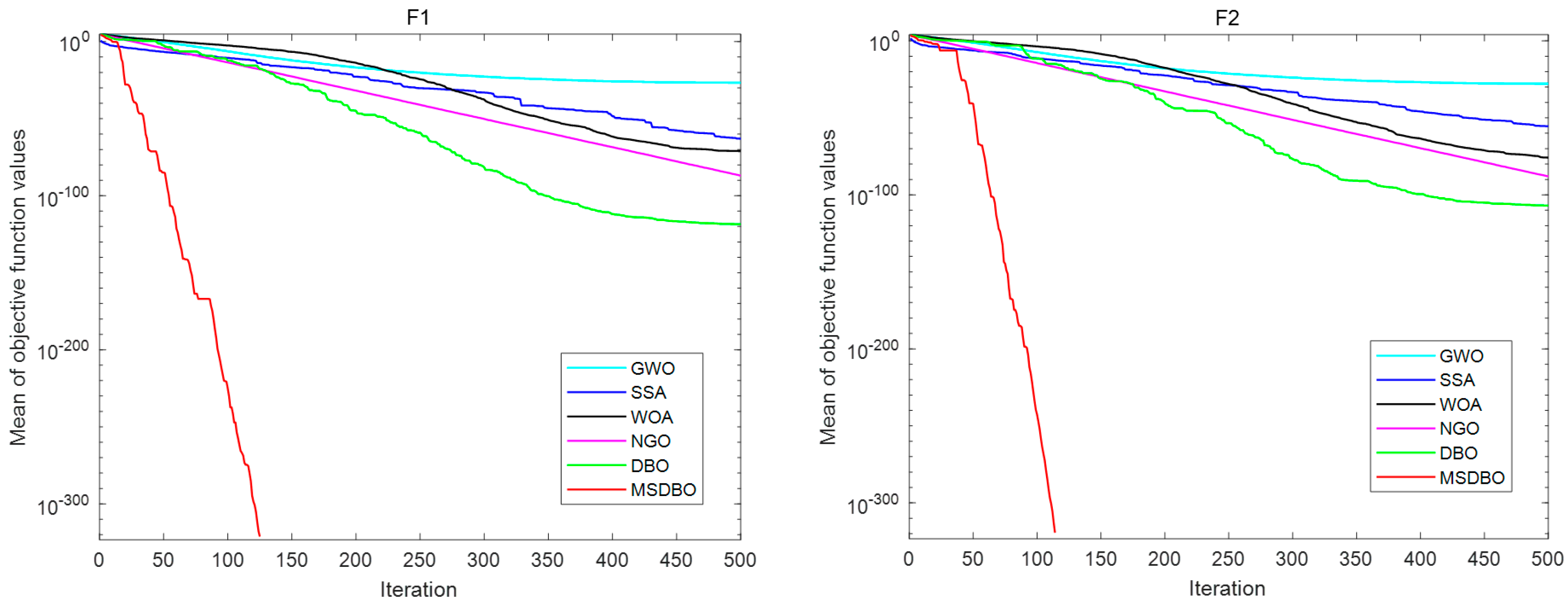
• A multi-strategy enhanced dung beetle optimizer (MSDBO), named the MSDBO–CNN–LSTM model for load forecasting, is proposed to adjust the hyperparameters of a CNN−LSTM. This adjustment enhances the model’s accuracy. Additionally, different optimization algorithms are compared to validate that the proposed MSDBO algorithm achieves the highest accuracy and the fewest iterations.
• Due to the difficulty of accurately analyzing the importance of various factors for transformer capacity-regulating control and the lack of weights on different factors, conventional fuzzy control methods perform poorly. For multifactor problems with unknown weights, hesitant fuzzy control combines the different opinions of multiple decision-makers for a more comprehensive analysis, resulting in decisions that are more relevant to the integrated opinions of multiple control. Compared to conventional fuzzy control, hesitant fuzzy control provides more accurate and comprehensive results.
• The effectiveness of the proposed capacity control method is assessed through simulation using the MATLAB/SIMULINK platform. The simulation results show that transformers using load forecasting models can accurately and promptly switch capacities. Transformers that combine load forecasting with hesitant fuzzy control can reduce the number of daily capacity switch operations while ensuring low power and economic losses.

The rest of this paper is organized as follows: Section 2 discusses the capacity-regulating principle of on-load capacity-regulating transformers. Section 3 introduces the CNN−LSTM model and the multi-strategy dung beetle optimization (MSDBO) algorithm. Through testing, it demonstrates the superiority of the MSDBO algorithm for optimization. Section 4 determines the regulating schemes for capacity nodes of transformers, introduces the use of hesitant fuzzy control, and presents an overall control strategy for on-load capacity regulation based on a combination of neural networks and fuzzy control. The case study is presented in Section 5. Finally, the conclusions and discussion are presented in Section 6.

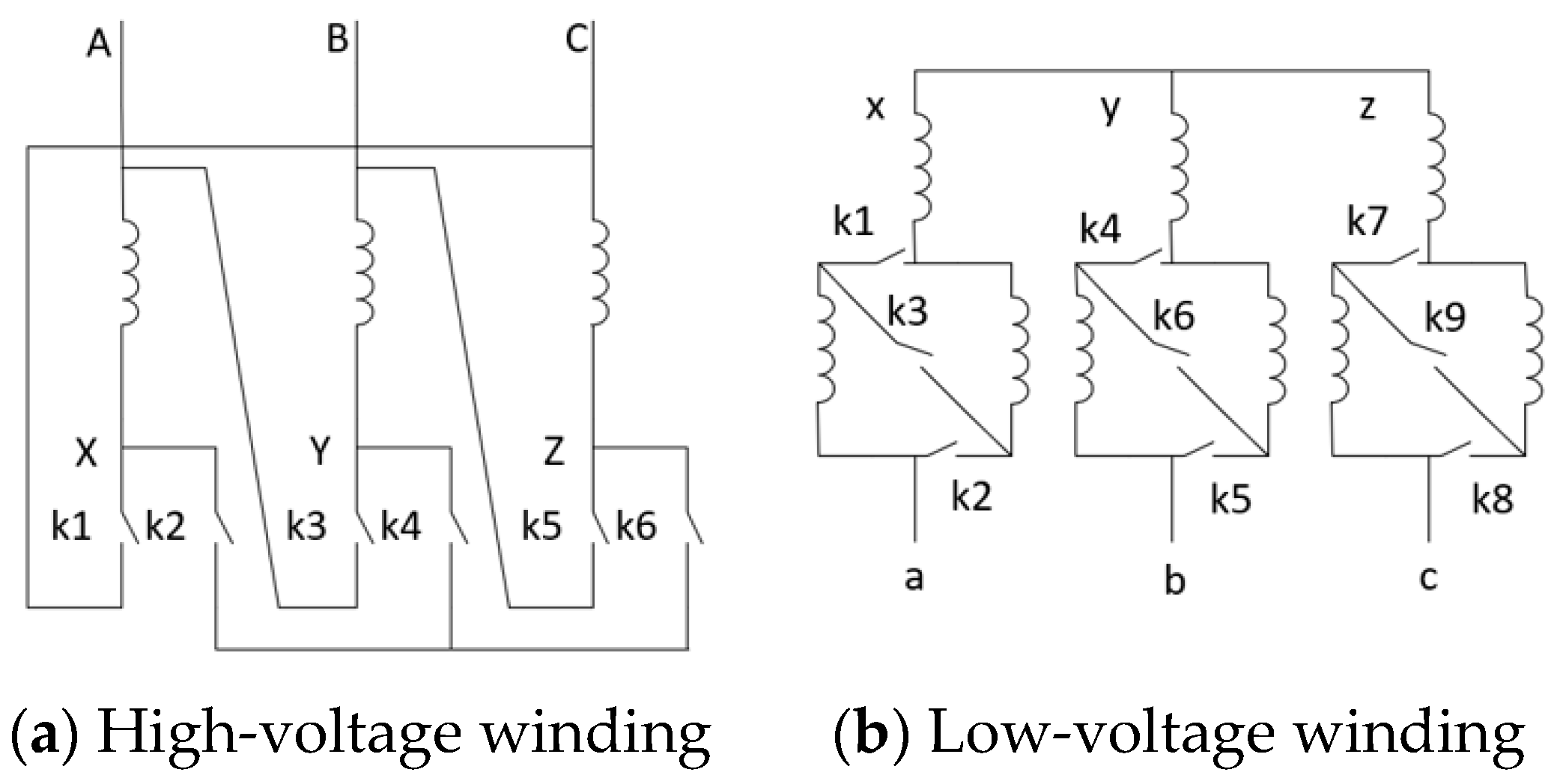
2. On-Load Capacity-Regulating Transformer Operating Principles

The study in this paper primarily focuses on on-load capacity-regulating transformers that employ a high-voltage winding star–delta transformation and a low-voltage winding series–parallel transformation, as illustrated in Figure 1. This capacity-regulating method is characterized by its effective loss reduction and widespread applicability. During the transformation of an OLCR transformer from low to high capacity, the number of turns in the low-voltage winding decreases. Simultaneously, the high-voltage winding changes to a Y connection, resulting in an increase in the phase voltage on the high-voltage side. The reduction in the number of turns and the increase in voltage are proportional, ensuring that the output voltage remains constant while the capacity is switched.

Figure 1a illustrates the high-voltage winding side. In this diagram, k1~k6 represent capacity-regulating switches. Figure 1b illustrates the low-voltage winding side. In this diagram, k1~k9 represent capacity-regulating switches.

When the high-voltage winding is connected in a delta configuration, and the low-voltage winding is connected in parallel with the second and third sections of the winding and in series with the first section of the winding, the transformer is in a high-capacity mode. On the other hand, when the high-voltage winding is connected in a star configuration and the low-voltage winding is connected in a series configuration with all three sections, the transformer operates in the low-capacity mode.

3. On-Load Capacity-Regulating Control Based on Load Forecasting

The existing OLCR transformer determines its operational state based on periodic monitoring of the load condition. It compares the determined state with its current state to decide whether the OLCR switch should be activated, thus controlling the OLCR switch operation. However, in situations where the load fluctuates frequently, the issue of delayed switch operation arises.

This chapter proposes an on-load transformer capacity-regulating control method based on MSDBO−CNN−LSTM (multi-strategy enhanced dung beetle optimizer—convolutional neural network—long short-term memory). The MSDBO−CNN−LSTM algorithm is employed for load forecasting and enhances prediction accuracy.

3.1. Load Forecasting Based on CNN−LSTM

The convolutional neural network (CNN) belongs to the category of feedforward neural networks, characterized by a deep structure and incorporating convolutional computations. The CNN comprises convolutional layers and pooling layers, utilizing convolutional computations to extract latent features from the data and employing pooling layers for downsampling and compression of network parameters. A one-dimensional CNN is employed in this study, and the architecture is illustrated in Figure 2.

The long short-term memory (LSTM) network is a variant of the recurrent neural network (RNN), specifically designed to mitigate the challenge of preserving long-term dependencies, a limitation often encountered in conventional RNNs. It enhances the basic RNN structure by introducing forget gates, input gates, and output gates, as shown in Figure 3. The LSTM network, through the incorporation of memory cells and gate mechanisms, is better equipped to capture and handle long-term dependencies within input sequences.

The forget gate, utilizing the input, the intermediate state, and the state memory unit, aims to retain useful information while avoiding the transmission of irrelevant information from the previous time step to the next. The roles of the input gate and the output gate include reading data and passing the processed data to the next time step. The computational formulas are presented as Formulas (1)–(6):

$$f_t=\sigma \left(H_{fx}{x}_t+H_{fh}{h}_{t-1}+b_f\right)$$

(1)

$$i_t=\sigma \left(H_{ix}{x}_t+H_{ih}{h}_{t-1}+b_i\right)$$

(2)

$$n_t=\varphi \left(H_{nx}{x}_t+H_{nh}{h}_{t-1}+b_n\right)$$

(3)

$$o_t=\sigma \left(H_{ox}{x}_t+H_{oh}{h}_{t-1}+b_o\right)$$

(4)

$$s_t=g_t\odot i_t+s_{t-1}\odot f_t$$

(5)

$$h_t=\varphi (s_t)\odot o_t$$

(6)

where $f_t$, $i_t$, $n_t$, $o_t$, $s_t$, and $h_t$ represent the states of the forget gate, input gate, input node, output gate, state unit, and intermediate output, respectively. $H_{fx}$, $H_{fh}$, $H_{ix}$, $H_{ih}$, $H_{nx}$, $H_{nh}$, $H_{ox}$, and $H_{oh}$ denote the matrix weights for the corresponding gates, input $x_t$, and intermediate input $h_{t-1}$. $b_f$, $b_i$, $b_n$, and $b_o$ are the bias terms for the respective gates. $\odot$ indicates element-wise multiplication in the vector, $\sigma$ represents the sigmoid function transformation, and $\varphi$ signifies the tanh function transformation.

The CNN–LSTM neural network combines CNN with LSTM. It utilizes input features such as the three-phase current amplitudes, three-phase voltage amplitudes, active power, reactive power, and oil temperature data for the transformer every half hour. The network is employed to predict the load on the transformer.

The predictive method consists of two parts: the CNN part for feature extraction and the LSTM part for load prediction. The CNN in this study comprises two convolutional layers, both of which are one-dimensional (Conv1D). The rectified linear unit (ReLU) is selected as the activation function for both convolutional layers. Following the convolutional layers, max-pooling operations are employed to downsample the features extracted by the convolutional layers, reducing the model parameters. There are also two layers of max-pooling (MaxPooling1D). After the two layers of convolution and pooling, the extracted vector arrays are passed as features to the LSTM network.

Through LSTM, the extracted features are thoroughly learned to capture the intrinsic relationships and periodic patterns among the data, enabling the prediction of future data. The LSTM network consists of one layer of LSTM with 48 neurons, using ReLU as the activation function. Finally, the output is passed through a fully connected layer (Dense) to generate a vector in the specified format.

3.2. The Multi-Strategy Enhanced Dung Beetle Optimizer

3.2.1. Dung Beetle Optimizer

Dung beetle optimizer (DBO) is an optimization algorithm grounded in the behavioral traits observed in dung beetles. This algorithm leverages five distinct behavioral characteristics exhibited by dung beetles—ball rolling, dancing, foraging, stealing, and reproduction—to acquire globally optimal weights and thresholds.

(1)

When the dung beetle encounters no obstacles, it navigates using the sun. The repositioning of the dung beetle rolling dung balls is influenced by

$$x_i(t+1)=x_i(t)+a\cdot k\cdot x_i(t-1)+b\cdot \left|x_i(t)-X^W\right|$$

(7)

where $t$ represents the number of iterations, $x_i(t)$ represents the position of the $i$th dung beetle, $a\in \left[0,1\right]$ represents the degree of offset caused by natural factors, $k\in \left[0,2\right]$ represents the perturbation coefficient $b\in \left[0,1\right]$, and $\left|x_i(t)-X^W\right|$ represents the change in light intensity, where a larger value indicates a lower light intensity and $X^W$ represents the worst position.

(2)

When a dung beetle encounters an obstacle and cannot move forward, it repositions itself through a dance, and its new position is updated to

$$x_i(t+1)=x_i(t)+\tan \theta \left|x_i(t)-x_i(t-1)\right|$$

(8)

where $\theta \in \left[0,\pi \right]$ represents the perturbation angle; when $\theta$ is 0 or $\frac{\pi }{2}$, the position remains unchanged. $\left|x_i(t)-x_i(t-1)\right|$ represents the offset of the $i$th dung beetle’s position.

(3)

The breeding area is simulated using a boundary selection strategy, defined as

$$x_i(t+1)=x_{gbest}(t)+g_1(x_i(t)-L_{g\ast })+g_2\left|x_i(t)-U_{g\ast }\right|$$

(9)

where $x_{gbest}(t)$ represents the global best position; $g_1$ and $g_2$ are two independent random vectors of size $1\times D$, where $D$ represents the dimension of the optimization problem; $L_{g\ast }$ and $U_{g\ast }$ represent the lower and upper bounds of the breeding area, respectively.

(4)

When dung beetles forage, the formula for position change is

$$x_i(t+1)=x_i(t)+C_1(x_i(t)-L_{g(t)})+C_2\left|x_i(t)-U_{g(t)}\right|$$

(10)

where $L_{g(t)}$ and $U_{g(t)}$ represent the lower and upper bounds of the foraging area, respectively, $C_1$ represents random numbers drawn from a normal distribution, and $C_2$ represents random vectors of size $1\times D$.

(5)

When dung beetles steal, the formula for position change is

$$x_i(t+1)=x_{lbest}(t)+Qf(\left|x_i(t)-x_{gbest}(t)\right|+\left|x_i(t)-x_{lbest}(t)\right|)$$

(11)

where $x_{lbest}(t)$ represents the best food source, $Q$ represents a constant value, and $f$ is a random vector of size $1\times D$ drawn from a normal distribution.

3.2.2. The Multi-Strategy Enhanced Dung Beetle Optimizer (MSDBO)

DBO is widely utilized for its simple structure and high accuracy. However, it is susceptible to becoming trapped in local optima, resulting in poor global optimization capabilities. To address this issue, this paper proposes a multi-strategy-enhanced DBO.

(1)

Bernoulli chaos mapping

The traditional DBO initializes the population positions using random number generation, which may not cover all positions in the environment, thus affecting the optimization effectiveness and convergence rate of the algorithm. Using Bernoulli chaotic mapping to explore as many positions in the environment as possible, the expression is given by

$$Z(t+1)=\left\{\begin{array}{ll}Z(t)/(1+\rho )\hfill & Z(t)\in \left(0,1-\rho \right]\hfill \\ \left(Z(t-1)+\rho \right)/\rho \hfill & Z(t-1)\in \left(1-\rho ,1\right)\hfill \end{array}\right.$$

(12)

where $Z(t)$ represents the current value of the chaotic sequence at the $t$th iteration and $\rho$ is the control coefficient. When $\rho =0.5$, the algorithm exhibits the best exploratory behavior.

(2)

Levy flight strategy

The Levy flight mechanism, which involves long-range, short-distance roaming, is beneficial for enhancing the diversity of the population. Long-range jumps with variable directions ensure detailed exploration of the nearby regions, and the mechanism’s mutation provides certain advantages for exploring a large space. By combining short-range and long-range flight modes, it reflects thorough optimization of the search space, thereby improving the algorithm’s global search capability.

If a dung beetle exhibiting stealing behavior becomes stuck in a local optimum, and its position update stagnates, applying the Levy flight strategy to update the individual’s position can help it escape from the local optimum and diffuse to more distant positions. The position is updated to

$$x_i(t+1)=x_i(t)+\alpha \oplus Levy(\lambda )$$

(13)

where $\alpha$ represents a random step length, $\oplus$ represents the dot product, and Levy is a random search path following the Levy distribution, constrained as follows:

$$Levy(\lambda )\sim \frac{\phi u}{{\left|v\right|}^{1/2}}$$

(14)

$$\phi ={\left[\frac{\Gamma (1+\lambda )\sin (\pi \lambda /2)}{\Gamma (1+\lambda /2)\lambda 2^{(\lambda -1)/2}}\right]}^{1/\lambda }$$

(15)

where $u$, $v$ follow a normal distribution and $\lambda =1.5$.

3.2.3. MSDBO Testing

To evaluate the effectiveness of the MSDBO algorithm, we selected test functions for performance testing and compared it with traditional algorithms, such as GWO, SSA, WOA, NGO, and DBO. The test functions included four unimodal functions and four multimodal functions, as shown in

Table 1. Test function.

Test Function	Value Range
$F_1\left(x\right)={\displaystyle \sum _{i=1}^n{x}_i^2}$	$\left[-100,\hspace{0.33em}100\right]$
$F_2\left(x\right)={\displaystyle \sum _{i=1}^{\mathrm{n}}\left|x_i\right|}+{\displaystyle \prod _{i=1}^n\left|x_i\right|}$	$\left[-10,\hspace{0.33em}10\right]$
$F_3\left(x\right)={{\displaystyle \sum _{i=1}^n\left({\displaystyle \sum _{j-1}^i{x}_j}\right)}}^2$	$\left[-100,\hspace{0.33em}100\right]$
$F_7\left(x\right)={\displaystyle \sum _{i=1}^{n}i{x}_i^4}+random\left[0,\left.1\right)\right.$	$\left[-1.28,\hspace{0.33em}1.28\right]$
$F_9\left(x\right)=\left[x_i^2-10\cos \left(2\pi x_i\right)+10\right]$	$\left[-5.12,\hspace{0.33em}5.12\right]$
$F_{10}\left(x\right)=-20\exp \left(-0.2\sqrt{\frac{1}{n}{\displaystyle \sum _{i=1}^n{x}_i^2}}\right)-\exp \left[\frac{1}{n}{\displaystyle \sum _{i=1}^n\cos \left(2\pi x_i\right)}\right]+20+e$	$\left[-32,\hspace{0.33em}32\right]$
$F_{11}\left(x\right)=\frac{1}{4000}\ast {\displaystyle \sum \left(x_i^2\right)-{\displaystyle \prod \left(\cos \left(\frac{x_i}{\sqrt{i}}\right)\right)}}+1$	$\left[-600,\hspace{0.33em}600\right]$
$F_{12}\left(x\right)=\frac{\pi }{n}\left\{10\sin \left(\pi y_1\right)+{\displaystyle \sum _{i=1}^{n-1}{\left(y_i-1\right)}^2}\left[1+10{\sin }^2\left(\pi y_{i+1}\right)\right]+{\left(y_n-1\right)}^2\right\}+{\displaystyle \sum _{i=1}^{n}u\left(x_i,10,100,4\right)}$	$\left[-50,\hspace{0.33em}50\right]$

.

Using MATLAB, simulation experiments were conducted on the test functions. To ensure fair comparison, the maximum number of iterations was uniformly fixed at 500, the population size was N = 30, and the dimension was D D = 30. Each algorithm was run 50 times, and the simulation results are shown in Figure 4.

From Figure 4, it can be observed that for both unimodal and multimodal functions, the MSDBO algorithm converges faster, achieves higher accuracy, and requires fewer iterations compared to other traditional algorithms. The optimal and average values obtained by the MSDBO algorithm are closer to the optimal value of the function, which demonstrates the significant advantages of the MSDBO algorithm used in this study over the other algorithms.

3.3. MSDBO−CNN−LSTM

To address the issue of local optima and improve the predictive performance of the CNN–LSTM neural network, this study utilizes the MSDBO algorithm to optimize the hyperparameters of the CNN−LSTM, such as the dropout rate and batch size. This optimization algorithm exhibits strong global search capabilities and fast convergence, effectively resolving the inherent problems of the CNN−LSTM. By applying the optimized hyperparameters to the CNN−LSTM, the optimization of the CNN−LSTM is achieved, resulting in more accurate load prediction results.

Figure 5 illustrates the architecture of the MSDBO−CNN−LSTM neural network.

4. On-Load Capacity Regulation and Optimization Based on Fuzzy Control

4.1. Calculation and Economic Analysis of Capacity-Regulating Nodes

The power loss of a transformer with different capacity levels is composed of no-load loss and short-circuit loss, as expressed by the following formula:

$$S_H=S_{OH}+{\beta }_H^2{S}_{XH}$$

(16)

$$S_L=S_{OL}+{\beta }_L^2{S}_{XL}$$

(17)

where $S_H$, $S_L$ represent the power loss for a transformer with different capacity levels, $S_{OH}$, $S_{OL}$ represent the no-load loss for a transformer with different capacity levels, ${\beta }_H$, ${\beta }_L$ represent the load factors for a transformer with different capacity levels, and $S_{XH}$, $S_{XL}$ represent the short-circuit loss for a transformer with different capacity levels.

$${\beta }_L=\frac{{\beta }_H{S}_{NH}}{S_{NL}}$$

(18)

where $S_{NH}$, $S_{NL}$ represent the rated capacity of the transformer for different capacity levels.

If we assume that $S_H=S_L$, meaning that the power loss is the same for different capacity levels, then, based on Formulas (16) and (17), the expression for the critical load can be obtained as follows:

$$S^{L-H}=\sqrt{\frac{P_{OH}-P_{OL}}{\frac{P_{XL}}{S_{NL}^2}-\frac{P_{XH}}{S_{NH}^2}}}$$

(19)

The operational cost calculation formula for the transformer is given by

$$C_y=[T_1\times (P_0+0.05\times I_0\times S_N/100)+T_2\times (P_x+0.05\times U_x\times S_N/100)]\times C$$

(20)

where $T_1$, $T_2$ represent the transformer no-load time and equivalent full-load time, respectively, $P_0$, $P_x$ represent the transformer no-load loss and load loss, respectively, $I_0$, $U_x$ represent the transformer no-load current and short-circuit impedance, respectively, and $S_N$, $C$ represent the transformer rated capacity and electricity price, respectively, where $C=0.5$ yuan/kWh and is a constant value.

The formula for calculating the power loss of a transformer is given by [16]:

$$\left\{\begin{array}{l}{P}_{0z}=P_0+K_Q{Q}_0+K_P{P}_0\\ P_{kz}=P_k+K_Q{Q}_k+K_P{P}_k\\ Q_0=I_0\%S_N/100\\ Q_k=U_k\%S_N/100\end{array}\right.$$

(21)

where $P_{0z}$, $P_{kz}$ represent no-load comprehensive loss and load comprehensive loss, respectively, $Q_0$, $Q_k$ represent no-load reactive power loss and short-circuit reactive power loss, respectively, $I_0\%$, $U_k\%$ represent no-load current and short-circuit impedance respectively, and $K_Q=0.1,K_p=0.2$.

4.2. Hesitant Fuzzy Control Making for Capacity-Regulating Nodes

The core idea of fuzzy control is to simulate human fuzzy reasoning and decision-making. By translating the expertise or experience of experts into fuzzy rules, it transforms real-time signals from sensors into fuzzy signals. These fuzzy signals are then used as inputs for fuzzy rules, and the output obtained from fuzzy reasoning is added to the actuator to achieve intelligent control of the system. The block diagram illustrating the principles is shown in Figure 6:

The fuzzy controller has inputs for switch times, power loss, and economic loss, and an output for adjustment node value. The domains and fuzzy subsets for each variable are as follows:

The number of switch changes: domain [0, 10], fuzzy subsets {LS (low), MS (medium), HS (high)};

Power loss: domain [0, 60], fuzzy subsets {LP (low), MP (medium), HP (high)};

Operating costs: domain [0, 30], fuzzy subsets {LC (low), MC (medium), HC (high)};

Switch taps: domain [30, 70], fuzzy subsets {VL (very low), L (low), M (medium), H (high), VH (very high)};

Triangular membership functions are used to describe the membership degrees of each variable, as shown in Figure 7.

Based on the fuzzy set relationships of switch changes, power loss, and operating costs, a more suitable switch node is determined. A fuzzy rule table is established accordingly, as shown in

Table 2. Fuzzy rule base.

			The Number of Switch Changes
			LS	MS	HS
Power loss and operating costs	LP	LC	VH	H	H
	LP	MC	H	H	M
	LP	HC	H	M	M
	MP	LC	H	H	M
	MP	MC	H	M	M
	MP	HC	M	M	L
	HP	LC	H	M	M
	HP	MC	M	M	L
	HP	HC	M	L	VL

.

Due to the difficulty in accurately analyzing the importance of various factors for transformer capacity-regulating control, and the lack of weights on different factors, conventional fuzzy control methods perform poorly. For multifactor problems with unknown weights, hesitant fuzzy control combines the different opinions of multiple decision-makers for a more comprehensive analysis, resulting in decisions that are more relevant to the integrated opinions of multiple decision-makers. Compared to conventional fuzzy control, hesitant fuzzy control provides more accurate and comprehensive results. The hesitant fuzzy control method is described in the following text:

Through factor $G=\left\{G_1,G_2,\cdots ,G_n\right\}$, decision-makers need to evaluate plan $A=\left\{A_1,A_2,\cdots ,A_m\right\}$, where n is the number of factors and m is the number of plans. Assuming $h_{ij}$ represents the evaluation by decision-makers of factor $G_j$ in option $A_i$, all $h_{ij}$ values constitute the hesitant fuzzy control matrix $H={\left(h_{ij}\right)}_{m\times n}$, $h_{ij}=\underset{t=1}{\overset{l_{ij}}{\cup }}\left\{{\gamma }_{ij}^{\left(t\right)}\right\}=\left\{{\gamma }_{ij}^{\left(1\right)},{\gamma }_{ij}^{\left(2\right)},\cdots {\gamma }_{ij}^{\left(t\right)}\right\}$, ${\gamma }_{ij}^{\left(t\right)}$ represents the $t$th evaluation value among $h_{ij}$. If the decision-maker’s attitude is comparatively optimistic, it will lead to missing values in the matrix. In the case of inconsistent lengths of hesitant fuzzy control elements, the maximum membership value should be added to the fewer elements to obtain the standardized matrix $\tilde{H}={\left({\tilde{h}}_{ij}\right)}_{m\times n}$. The weight vector $\lambda$ represents the relative importance of the factors, i.e., $\lambda ={\left({\lambda }_1,{\lambda }_2,\cdots ,{\lambda }_n\right)}^T$, satisfying the formula ${\lambda }_j\in \left[0,1\right],{\displaystyle {\sum }_{j=1}^n{\lambda }_j=1}$. The operator-related weight vector $\omega ={\left({\omega }_1,{\omega }_2,\cdots ,{\omega }_n\right)}^T$ satisfies the formula ${\omega }_j\in \left[0,1\right],{\displaystyle {\sum }_{j=1}^n{\omega }_j=1}$.

The factor weight represents the relative importance of the factors and the preferences of the decision-maker. Due to the unknown weight coefficients, the hesitant fuzzy hamming distance is used to extend the maximum deviation method to the hesitant control environment, obtaining the optimal weight vector $\lambda ={\left({\lambda }_1,{\lambda }_2,\cdots ,{\lambda }_n\right)}^T$.

$${\lambda }_j=\frac{Y_j}{{\displaystyle {\sum }_{j=1}^n{Y}_j}},j=1,2,\cdots ,n,$$

(22)

where $Y_j={\displaystyle \sum _{i=1}^m{\displaystyle \sum _{k=1}^m\left(\frac{1}{l}{\displaystyle \sum _{t=1}^l\left|{\tilde{\gamma }}_{ij}^{(t)}-{\tilde{\gamma }}_{kj}^{(t)}\right|}\right)}},j=1,2,\cdots ,n.$

The operator-related weight vector is an important part of the generalized hesitant fuzzy mixed-weighted aggregation operator used for information integration. In this paper, the operator-related weight vector $\omega ={\left({\omega }_1,{\omega }_2,\cdots ,{\omega }_n\right)}^T$ is determined using a normal distribution.

Table 3. The variation of $\omega$ for n ranging from 2 to 5.

n	Operator-Related Weight Vector $\mathit{\omega }={\left({\mathit{\omega }}_1,{\mathit{\omega }}_2,\cdots ,{\mathit{\omega }}_{\mathit{n}}\right)}^{\mathit{T}}$
2	$\omega ={\left(0.5,0.5\right)}^T$
3	$\omega ={\left(0.2429,0.5142,0.2429\right)}^T$
4	$\omega ={\left(0.1550,0.3450,0.3450,0.1550\right)}^T$
5	$\omega ={\left(0.1117,0.2365,0.3036,0.2365,0.1117\right)}^T$

shows the variation of $\omega$.

For the hesitant fuzzy multifactor control method under unknown weights, the algorithm proceeds as follows:

(1)

Generate the hesitant fuzzy control matrix $H={\left(h_{ij}\right)}_{m\times n}$ based on the decision-maker’s evaluations of the options, and obtain matrix $\tilde{H}={\left({\tilde{h}}_{ij}\right)}_{m\times n}$ by standardizing the matrix.

(2)

Calculate the optimal weight vector $\lambda ={\left({\lambda }_1,{\lambda }_2,\cdots ,{\lambda }_n\right)}^T$ based on Formula (12).

(3)

Select the operator-related weight vector $\omega ={\left({\omega }_1,{\omega }_2,\cdots ,{\omega }_n\right)}^T$ based on the value of n.

(4)

Using the new hesitant fuzzy control weighted aggregation operator (NGHFHWA), integrate ${\tilde{h}}_{ij}$ into the hesitant fuzzy element ${\tilde{h}}_i$ for each option $A_i$.

$${\tilde{h}}_i=NGHFHWA({\tilde{h}}_{i1},{\tilde{h}}_{i2},\cdots {\tilde{h}}_{in})$$

(23)

(5)

Calculate the score function $S({\tilde{h}}_i)$ based on ${\tilde{h}}_i$. If the score functions are equal, differentiate them through the hesitant fuzzy-order central aggregation function $p({\tilde{h}}_i)$ for sorting.

$$s(h)=\frac{1}{l}{\displaystyle \sum _{i=1}^l{\gamma }^{\left(i\right)}}$$

(24)

(6)

Arrange the options according to the score function $S({\tilde{h}}_i)$ and then choose the one with the highest score as the best option.

The hesitant fuzzy control process diagram is illustrated in Figure 8:

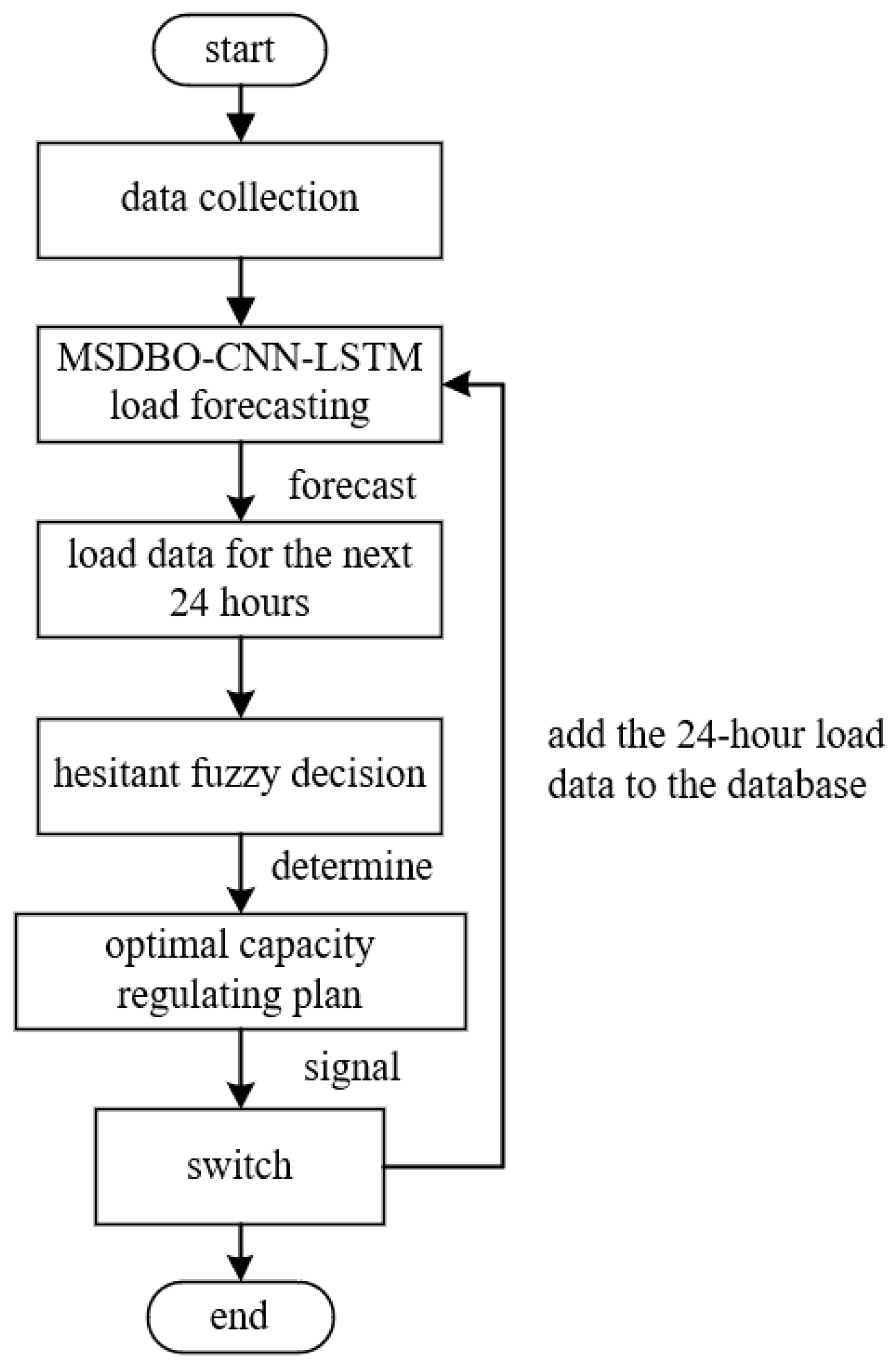
5. On-Load Capacity-Regulating Control Strategy and Methodology

The variation in load leads to changes in data, such as current, voltage, and active power. Capacity regulation of the transformer can be achieved through sensor monitoring and feedback. However, this type of capacity-regulating method relies heavily on real-time data, lacks adaptability to learning from data, and cannot provide warnings for future load conditions over a certain period.

To address the above issues, this study employs an MSDBO−CNN−LSTM neural network to predict load data for the next 24 h. Based on these data, suitable capacity-regulating schemes are selected through hesitant fuzzy control. The merit values for switch operation frequency, power losses, and operating costs are calculated, and a weighted sum is used to determine the comprehensive merit value for each scheme. The optimal capacity-regulating scheme is then identified. Control of the capacity-regulating switches is carried out using a step wave signal. Additionally, the load data for this time are added to the database for use in the next round of MSDBO−CNN−LSTM predictions, ensuring the real-time and accurate nature of subsequent forecasting results.

This study proposes a method for the capacity adjustment of OLCR transformers in distribution networks using a combination of load prediction and hesitant fuzzy control, as shown in Figure 9. The methodology consists of the following steps:

• Step 1. Data collection:

Collect historical load data from the distribution network, including daily load profiles, for analysis and prediction. The load data should encompass various periods to capture seasonal variations and different operational scenarios.

• Step 2. Load forecasting:

Preprocess the historical load data to ensure its quality and consistency. Utilize the MSDBO−CNN−LSTM model to predict future load demand based on historical data.

• Step 3. Hesitant fuzzy control:

  (1)

  Define the evaluation criteria for selecting the optimal adjustment scheme, including the number of switch times, power losses, and operating costs.

  (2)

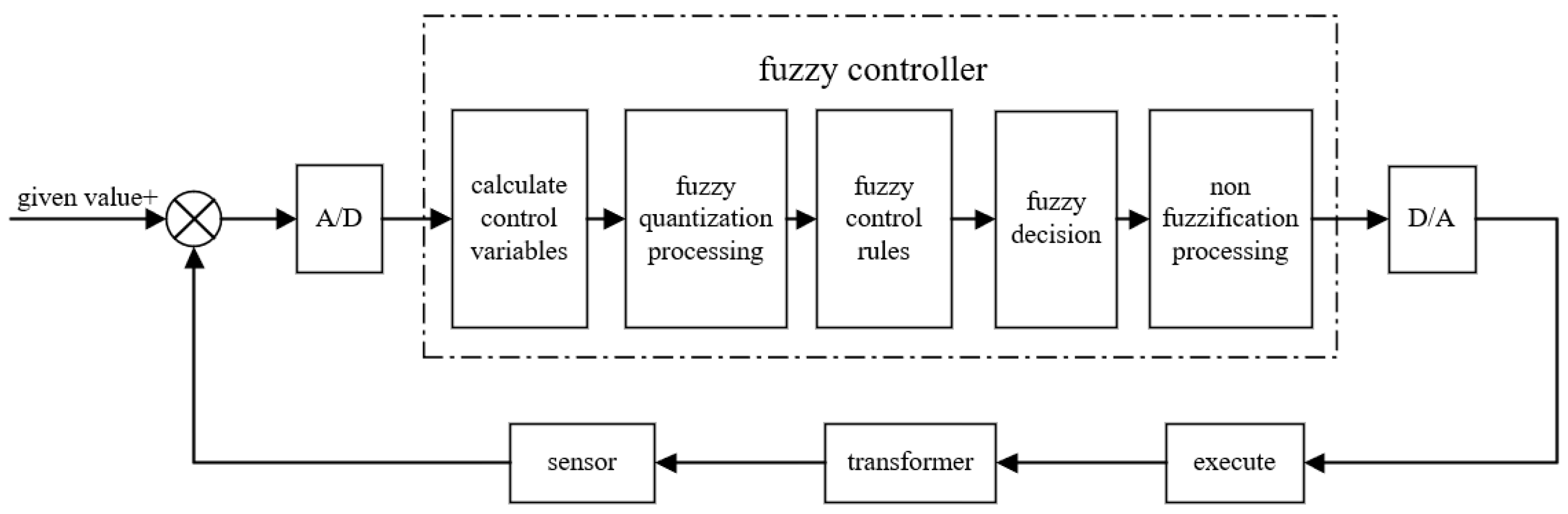
  Design a fuzzy controller with inputs of the number of switch changes, power loss, and operating costs, and an output of adjustment node value.

  (3)

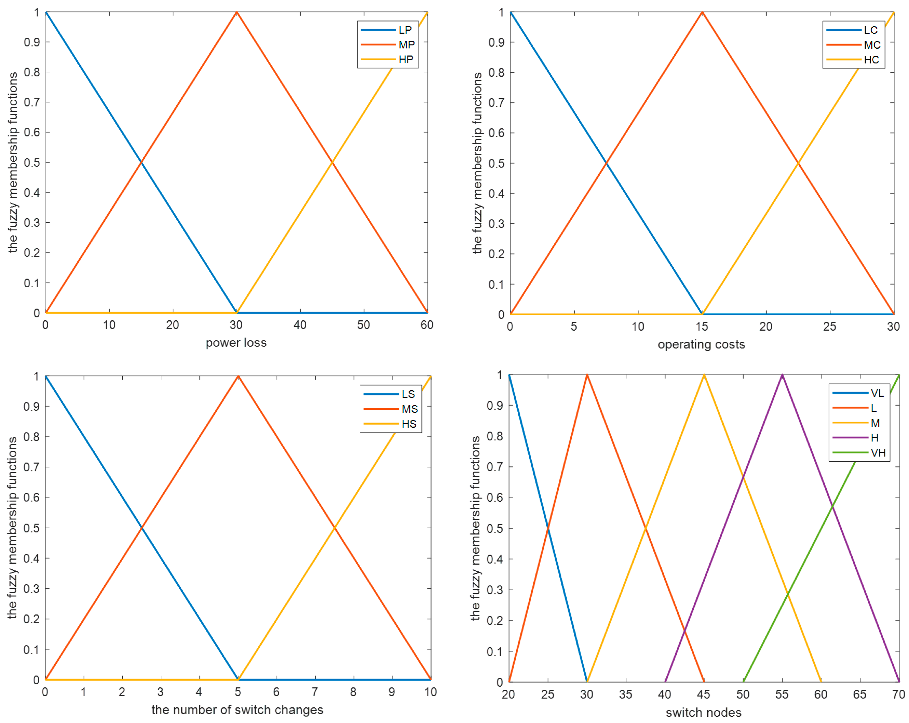
  Define the fuzzy subsets and membership functions for each input and output variable.

  (4)

  Develop fuzzy rules based on expert knowledge and the fuzzy rule base table to determine the adjustment node value.

• Step 4. Optimal capacity-regulating plan:

  (1)

  Develop a detailed capacity adjustment schedule for the 24-h period based on the optimal adjustment nodes obtained through load forecasting and hesitant fuzzy decision-making methods.

  (2)

  Reduce power losses and operating costs through the capacity adjustment schedule while minimizing the number of switch changes as much as possible.

• Step 5. Action and analysis:

  (1)

  Control the switching of OLCR transformer capacity by implementing the optimal capacity-regulating plan in the form of signals.

  (2)

  Compare the performance of the conventional OLCR transformer with the proposed method in terms of the number of switching times, power losses, and operating costs.

  (3)

  Analyze the results of different scenarios to demonstrate the effectiveness and superiority of the proposed method in capacity regulation.

6. Case Studies and Results Analysis

6.1. Example Introduction

According to the principles of OLCR transformers, simulation models are constructed using the MATLAB/SIMULINK platform. Figure 10a is a diagram illustrating the regulation of transformer capacity based on real-time load currents. Figure 10b is a diagram of a transformer capacity-regulating control using an MSDBO−CNN−LSTM neural network and hesitant fuzzy control.

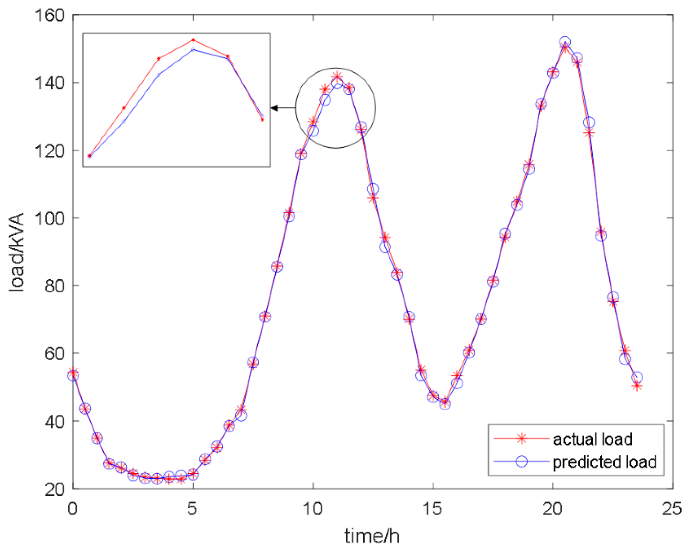
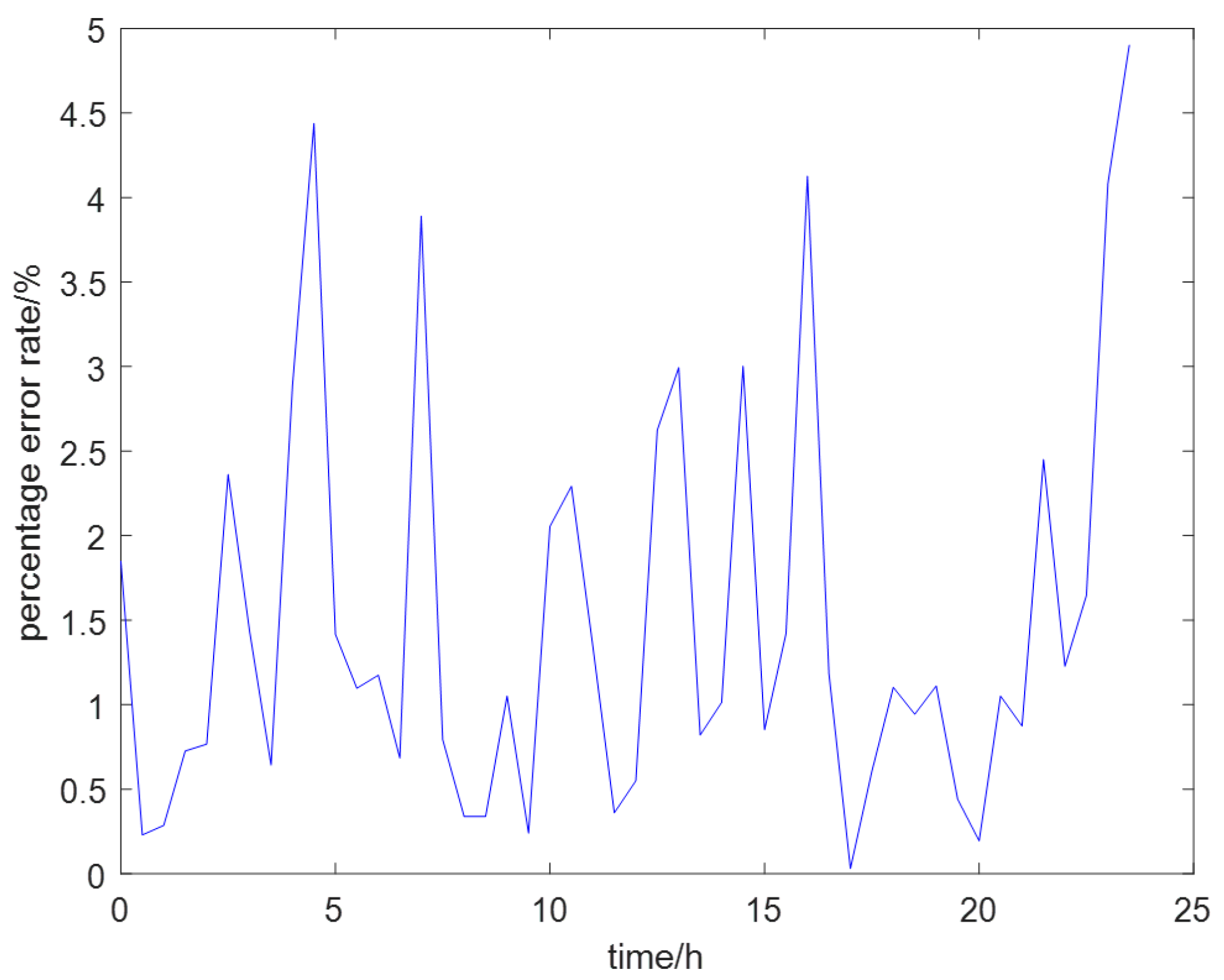
6.2. Load Forecasting Based on an MSDBO−CNN−LSTM Model

Using an MSDBO−CNN−LSTM neural network, the next 24 h of data are predicted, and Figure 11 presents a comparative graph between the predicted results and the actual values over the 24-h period.

The relative error between the actual and predicted results for the 24-h load is presented, as shown in Figure 12.

From the graph, it can be observed that the relative errors are all less than 5%.

$R^2$ is the coefficient of determination, an accuracy evaluation metric in machine learning. In this case, the obtained $R^2$ value is 0.9789.

6.3. Capacity-Regulating Control Based on Hesitant Fuzzy Control

Choosing the S11-M series three-phase transformer with a rated capacity of 315/100 kVA, the critical load is calculated by substituting the data from

Table 4. S11-M three-phase transformer operating parameters.

Rated Capacity (kVA)	No-Load Loss (kW)	Load Loss (kW)	No-Load Current (%)	Short-Circuit Impedance (%)	Critical Value (kVA)
315/100	0.48	3.65	1.1	4	49.73
	0.2	1.5	1.6	4

into Formula (19).

The calculation results from the table above indicate that 49.73 kVA is the transformer’s critical load. The transformer runs in low-capacity mode when the load is less than 49.73 kVA. On the other hand, the transformer goes into high-capacity mode when the load surpasses 49.73 kVA. Power loss is reduced and economic efficiency is increased by switching between these two capacity modes.

To calculate the daily operational cost through exemplification, the measured load data of a transformer on a specific day are considered. Within the course of that day, the transformer operated at reduced capacity for a total of 8 h and at full capacity for 16 h.

The following results are obtained through the calculation using Formula (20), as shown in

Table 5. Daily operating costs of three-phase transformers.

Rated Capacity (kVA)	Operating Cost of the OLCR Transformer (CNY)	Rated Capacity (kVA)	Operating Cost of the Fixed-Tap Transformer (CNY)	Cost Savings with OLCR Transformer (CNY)	Cost Savings with OLCR Transformer (%)
315/100	16.61	315	20.68	4.07	19.68

.

The load data for a transformer over the course of one year is considered, during which the transformer operates at reduced capacity for a total of 6108 h and at full capacity for 2532 h.

The following results are obtained through the calculation using the above Formula (20), as shown in

Table 6. Annual operating cost of three-phase transformers.

Rated Capacity (kVA)	Operating Cost of the OLCR Transformer (CNY)	Rated Capacity (kVA)	Operating Cost of the Fixed-Tap Transformer (CNY)	Cost Savings with OLCR Transformer (CNY)	Cost Savings with OLCR Transformer (%)
315/100	4334.80	315	8240.50	3905.70	47.40

.

In the provided data, the maximum load over the course of a year is 200 kVA. If a transformer with a rated capacity of 250 kVA, such as the S11-M-250/10 model, were employed, the daily operational cost for the transformer would be 19.025 yuan, resulting in a cost saving of 12.69%. Furthermore, the annual operational cost for the transformer would amount to 6859.3 yuan, leading to a cost saving of 36.8%.

After performing calculations and economic analyses of the switching capacity nodes, the selection of these nodes can be initiated through hesitant fuzzy control. Based on the following three factors, choose the appropriate regulating scheme, where $G_1$ represents the number of switch changes, $G_2$ represents power loss, and $G_3$ represents operating costs. Suppose there are three regulating schemes $A_i(i=1,2,3)$ to choose from, with capacity nodes of 40 kVA, 50 kVA, and 60 kVA, respectively. Due to the difficulty of precisely analyzing the importance of the three factors, it is challenging to directly decide which scheme to choose. By using hesitant fuzzy sets to represent the evaluation values of each scheme relative to the three factors, the hesitant fuzzy control matrix $H={\left(h_{ij}\right)}_{3\times 3}$ can be obtained, as shown in

Table 7. Hesitant fuzzy control matrix.

	G1	G2	G3
$A_1$	{0.7, 0.8, 0.9}	{0.4, 0.6}	{0.5, 0.6, 0.7}
$A_2$	{0.5, 0.6}	{0.7, 0.8, 0.9}	{0.4, 0.5}
$A_3$	{0.3, 0.4, 0.5}	{0.6, 0.7}	{0.7, 0.8}

.

After standardizing the matrix, the matrix $\tilde{H}={\left({\tilde{h}}_{ij}\right)}_{3\times 3}$ is obtained as shown in

Table 8. Standardize the hesitant fuzzy control matrix.

	G1	G2	G3
$A_1$	{0.7, 0.8, 0.9}	{0.4, 0.6, 0.6}	{0.5, 0.6, 0.7}
$A_2$	{0.5, 0.6, 0.6}	{0.7, 0.8, 0.9}	{0.4, 0.5, 0.5}
$A_3$	{0.3, 0.4, 0.5}	{0.6, 0.7, 0.7}	{0.7, 0.8, 0.8}

.

According to Table 2, when n = 3, $\omega ={\left(0.2429,0.5142,0.2429\right)}^T$.

Using Formula (22), the factor weight vector can be obtained as $\lambda ={\left(0.4138,0.2759,0.3103\right)}^T$.

For the capacity-regulating schemes $A_1$, $A_2$, and $A_3$, the corresponding ${\tilde{h}}_i$ can be calculated using the NGHFHWA operator. This paper takes $A_1$ as an example.

$$\begin{array}{l}{\tilde{h}}_1=NGHFHWA({\tilde{h}}_{11},{\tilde{h}}_{12},{\tilde{h}}_{13})\\ =NGHFHWA(\left\{0.7,0.8,0.9\right\},\left\{0.4,0.6,0.6\right\},\left\{0.5,0.6,0.7\right\}\end{array}$$

According to the formula, it can be concluded that $s({\tilde{h}}_{11})=\frac{0.7+0.8+0.9}{3}=0.8$, $s({\tilde{h}}_{12})=\frac{0.4+0.6+0.6}{3}=0.5333$, $s({\tilde{h}}_{13})=\frac{0.5+0.6+0.7}{3}=0.6$.

At this point, ${\tilde{h}}_{11}>{\tilde{h}}_{13}>{\tilde{h}}_{12}$. According to the normal distribution of $\omega$, it can be inferred that ${\omega }_1^{\prime }={\left(0.2429,0.2429,0.5142\right)}^T$. Using this information, the following calculation can be carried out:

$$\frac{{\lambda }_1{\omega }_{11}^{\prime }}{{\displaystyle {\sum }_{j=1}^3{\lambda }_j{\omega }_{1j}^{\prime }}}=0.3073,\frac{{\lambda }_2{\omega }_{12}^{\prime }}{{\displaystyle {\sum }_{j=1}^3{\lambda }_j{\omega }_{1j}^{\prime }}}=0.2049,\frac{{\lambda }_3{\omega }_{13}^{\prime }}{{\displaystyle {\sum }_{j=1}^3{\lambda }_j{\omega }_{1j}^{\prime }}}=0.4878.$$

When $p=1$, perform the following calculation.

$$\begin{array}{l}{\tilde{h}}_1=NGHFHWA({\tilde{h}}_{11},{\tilde{h}}_{12},{\tilde{h}}_{13})\\ ={\displaystyle \underset{i=1}{\overset{3}{\cup }}\left\{{\left(1-{\left(1-{\left({\tilde{\gamma }}_{11}^{(i)}\right)}^p\right)}^{0.3073}{\left(1-{\left({\tilde{\gamma }}_{12}^{(i)}\right)}^p\right)}^{0.2049}{\left(1-{\left({\tilde{\gamma }}_{13}^{(i)}\right)}^p\right)}^{0.4878}\right)}^{\frac{1}{p}}\right\}}\\ =\left\{0.5544,0.6749,0.7711\right\}\end{array}$$

Using the same method, the hesitant fuzzy elements ${\tilde{h}}_2=\left\{0.5280,0.5308,0.6771\right\}$ and ${\tilde{h}}_3=\left\{0.5540,0.6607,0.6797\right\}$ synthesized from $A_2$ and $A_3$, respectively, can be calculated.

For the capacity-regulating schemes $A_1$, $A_2$, and $A_3$, the respective score values $s({\tilde{h}}_i)$ are calculated as follows:

$$s({\tilde{h}}_1)=0.6668,s({\tilde{h}}_2)=0.5786,s({\tilde{h}}_3)=0.6315.$$

Based on the score values $s({\tilde{h}}_i)$, the capacity regulating schemes $A_1$, $A_2$, and $A_3$ are ranked in the following order: $A_1>A_3>A_2$. Therefore, $A_1$ is the best capacity-regulating scheme.

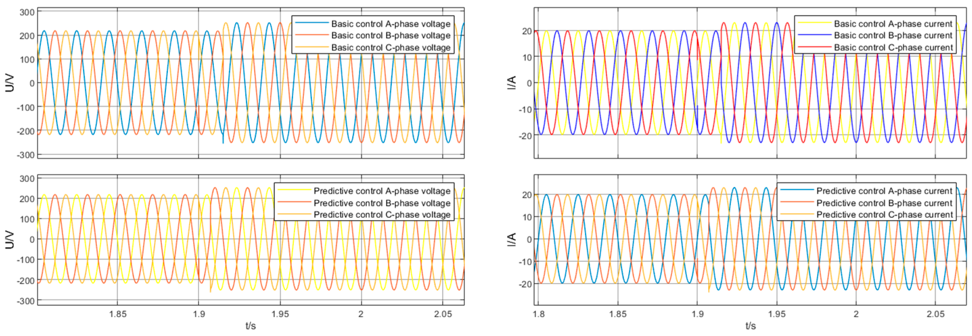
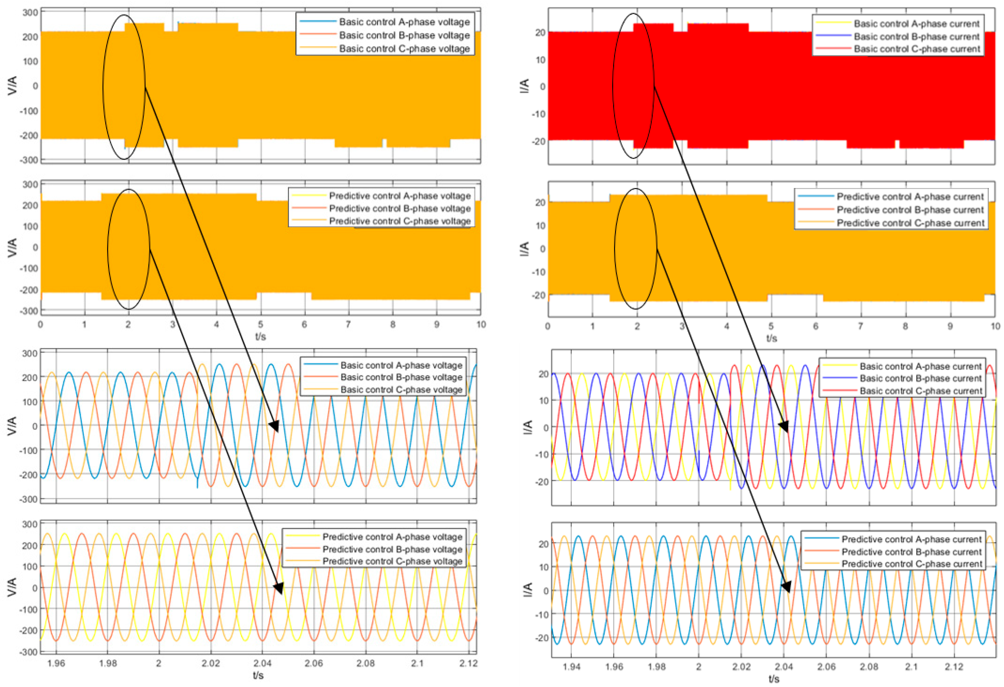
6.4. Simulation Results and Analysis

In the experiment of this paper, the three-phase transformer is formed by three multi-winding single-phase transformer models, with parameters set to have one primary winding and three secondary windings (one 27% turn and two 73% turn windings), achieving an S11-M 350/100 kVA capacity-adjustable distribution transformer. All transformer parameter settings are consistent, with $S_N=100$ kVA, $U_1/U_2=5774/220$ V, high and low voltage side 4-section winding resistance per unit values of 0.075, 0.041, 0.041, and 0.028, respectively, leakage reactance per unit values for each section of 0.02, 0.11, 0.11, and 0.08, respectively, and excitation impedance per unit values of 50, 50, respectively. In this study, the voltage source in this simulation is provided by a three-phase generator. The three-phase generator has a rated power of 320 kW for main use and 350 kW for standby, operating at a speed of 1500 rpm. It has a power factor of 0.8 and a rated voltage of 400/230 V. The peak amplitude of an ideal sinusoidal AC voltage source is 5774 V with a frequency of 50 Hz, and each phase is 120 degrees apart.

To simulate the capacity-regulating transformer SIMULINK model, the initial state assumes that the transformer is in a reduced capacity state. At 1.9 s, when the load capacity exceeds 49.73 kVA, the transformer switches to a full-capacity state.

Figure 13 illustrates the voltage and current waveforms for the A−, B−, and C−phases for both the conventional OLCR transformer and the load prediction-controlled OLCR transformer.

At 1.9 s, when the capacity state switches, no significant fluctuation is observed in the voltage and current in the A−, B−, and C−phases. This indicates that, after the capacity switch, the output voltage and current of the capacity-regulating transformer remain relatively stable. The capacity-regulating transformer controlled by load prediction demonstrates the ability to switch between the reduced and full capacities accurately and rapidly. As shown in the figure, the load forecasting control switches in a more timely fashion than in a conventional OLCR transformer. This is because the conventional OLCR transformer makes judgments on capacity regulation at fixed intervals, while predictive control involves real-time prediction and judgment for switching, making it capable of faster capacity regulation.

Based on load forecasting, fuzzy control is employed to evaluate the comprehensive merit values of multiple scenarios using switch-switching frequency, power loss, and operational cost as fuzzy control criteria.

The optimal variable-capacity-regulating scheme is selected, and after incorporating it into the simulation, the voltage and current waveforms for the A−, B−, and C−phases are obtained, as shown in Figure 14. With reasonable capacity regulation, the number of switching operations for the transformer is reduced from eight to four, avoiding frequent switching actions and achieving the goal of hesitant fuzzy control.

6.5. Scene Analysis

To test the effectiveness and reliability of the proposed method, this paper selects three different scenarios for analysis, as detailed below:

(1)

Scenario 1: During the busy agricultural season, electricity consumption in rural power grids is concentrated, leading to significant load fluctuations and severe overloading of transformers.

(2)

Scenario 2: During the idle agricultural season, electricity consumption in rural power grids is more dispersed. Transformers operate in no-load or light-load conditions for extended periods, leading to higher no-load losses.

(3)

Scenario 3: Urban residents’ electricity consumption follows daily life rhythms, resulting in large peak–valley differences in electricity usage.

For each of the three scenarios, the MSDBO−CNN−LSTM model is used to make predictions, resulting in 10 sets of 24−h predicted data for this scenario. Ten sets of 24−h actual data are selected to simulate the conventional OLCR transformer, and 10 sets of 24−h predicted data are selected to simulate the OLCR transformer based on the method proposed in this paper. The simulation results are analyzed to validate the superiority of the method proposed in this paper under each operating scenario.

MATLAB/SIMULINK simulations using data from September to October are conducted, corresponding to the busy agricultural season. The simulations are used to calculate the daily operating costs, power loss, and number of switch changes for the transformer. The results from the ten sets of calculations are used to compare the performance of the conventional OLCR transformer and the OLCR transformer based on load prediction and hesitant fuzzy decision-making. A S11−M 315/100kVA OLCR transformer is selected for this scenario. The results are shown in

Table 9. Results of 10 cases in the busy agricultural season.

Case	The Number of Switch Changes		Power Loss (kWh)		Operating Costs (CNY)
	Conventional Method	New Method	Conventional Method	New Method	Conventional Method	New Method
1	2	1	17.6	19.2	10.9	11.8
2	2	1	21.2	23.4	12.6	14.0
3	4	3	31.7	33.6	18.0	19.3
4	1	1	16.7	19.1	10.3	11.7
5	4	3	34.5	36.8	19.3	20.8
6	4	2	30.5	32.1	17.3	18.5
7	3	1	25.6	27.5	14.9	16.2
8	3	1	27.4	29.4	15.8	17.2
9	2	1	20.8	21.8	12.4	13.1
10	3	2	25.0	28.1	14.5	16.4

.

Calculating the average of the results from the 10 cases can provide a better overall analysis of the effectiveness and superiority of the proposed method in this paper.

Table 10. Average results for the busy agricultural season.

	The Number of Switch Changes	Power Loss (kWh)	Operating Costs (CNY)
Fixed-tap transformer	/	37.9	21.3
Conventional method	2.8	25.1	14.6
New method	1.6	27.1	15.9

compares the various results of the fixed-tap transformer, the OLCR transformer controlled by the traditional method, and the OLCR transformer controlled by the new method proposed in this paper.

Ten sets of 24−h data from March for the idle agricultural season are used to simulate and verify the conventional OLCR transformer and the OLCR transformer based on the method proposed in this paper, following the same validation method used for the busy agricultural season scenario. A S11−M 315/100kVA OLCR transformer is selected for this scenario. The results are shown in

Table 11. Average results for the idle agricultural season.

	The Number of Switch Changes	Power Loss (kWh)	Operating Costs (CNY)
Fixed-tap transformer	/	84.3	42.1
Conventional method	6.3	33.7	19.2
New method	2.7	36.8	20.7

.

Similarly, for the urban residents’ electricity consumption scenario, 10 sets of 24−h data are randomly selected from the entire year for simulation and verification of both the conventional OLCR transformer and the OLCR transformer based on the method proposed in this paper. A S11−M 400/125kVA OLCR transformer is selected for this scenario. The results are shown in

Table 12. Average results of urban residents.

	The Number of Switch Changes	Power Loss (kWh)	Operating Costs (CNY)
Fixed-tap transformer	/	58.5	29.2
Conventional method	3.7	29.8	17.2
New method	2.1	31.1	17.8

.

The following conclusions can be drawn from the above scenarios:

(1)

Both the conventional OLCR transformer and the OLCR transformer controlled by the method proposed in this paper can effectively reduce power loss and operating costs, with the reduction effect significantly increasing as the load decreases. For the idle agricultural season in rural power grids, using the method proposed in this paper reduces daily power loss and daily economic loss by an average of 56.3% and 50.8%, respectively. For the busy agricultural season in rural power grids, using the method proposed in this paper reduces daily power loss and daily economic loss by an average of 28.5% and 25.4%, respectively. For urban residents’ electricity consumption, using the method proposed in this paper reduces daily power loss and daily economic loss by an average of 46.8% and 39%, respectively.

(2)

Compared to a conventional OLCR transformer, an OLCR transformer controlled by load prediction and fuzzy hesitant decision-making can significantly reduce the daily number of switch operations while sacrificing some loss reduction capability. For the three scenarios mentioned above, the method used in this paper can sacrifice 3.5% to 9.2% of the loss reduction capability in exchange for reducing the number of switch operations by 28.6% to 57.1%. This significantly extends the lifespan of the switches, thereby increasing the operational lifespan of the transformer.

7. Conclusions

The control method proposed in this paper enables OLCR transformers to effectively address operating conditions, such as no-load, light-load, overload, and voltage fluctuations caused by load fluctuations, which is of great significance for building energy-efficient and smart grids. This paper utilizes the MSDBO−CNN−LSTM neural network to predict the load situation, calculates the switch node based on transformer parameters, and analyzes its economic feasibility. By employing hesitant fuzzy control to select the optimal switch node, a SIMULINK model for OLCR transformers is constructed and simulated. Experimental validation demonstrates the superiority of this method in different electrical scenarios, leading to the following conclusions:

(1)

The utilization of an MSDBO−CNN−LSTM neural network in this study for forecasting the load conditions for the next 24 h enables accurate switching of the transformer capacity mode. This helps avoid prolonged periods of overload or light-load conditions for the transformer. By reducing losses, it extends the operational lifespan of the on-load variable transformer, thereby enhancing the security and stability of the power grid.

(2)

In this study, a hesitant fuzzy control approach is employed to select the variable-capacity regulating nodes. Considering the three major factors of loss, economy, and switching frequency, the approach aims to minimize power loss and operating cost while reducing the number of switching operations. This strategy helps avoid a decrease in the operational lifespan of the transformer due to frequent capacity switch operations.

(3)

This control method demonstrates good capacity adjustment effects for OLCR transformers in rural distribution networks with seasonal loads and in urban residential networks with symmetric loads. It is applicable in various scenarios and exhibits superior performance. For the three scenarios mentioned above, the method reduces daily power loss by 28.5% to 56.3% and daily operating costs by 25.4% to 50.8%. The method used in this paper can sacrifice 3.5% to 9.2% of the loss reduction capability in exchange for reducing the number of switch operations by 28.6% to 57.1%. This significantly extends the lifespan of the switches, thereby increasing the operational lifespan of the transformer.

The work presented in this paper focuses on the analysis of the losses and economics of distribution transformers under balanced three-phase scenarios. In future work, the authors plan to conduct further research on the transformer adjustment strategy under three-phase unbalanced scenarios.

References

1. Zhang, W.; Jiang, J.; Li, B. Residual lifetime evaluation of power transformers based on data fusion and wiener model. IEEE Trans. Power Deliv. 2023, 38, 4189–4201. [Google Scholar] [CrossRef]
2. Yao, D.; Li, L.; Zhang, S.; Zhang, D.; Chen, D. The vibroacoustic characteristics analysis of transformer core faults based on multi-physical field coupling. Symmetry 2022, 14, 544. [Google Scholar] [CrossRef]
3. Wang, S.; Gao, M.; Zhuo, R. Research on high efficient order reduction algorithm for temperature coupling simulation model of transformer. High Volt. Appar. 2023, 59, 115–126. [Google Scholar]
4. Chen, T.; Chen, Y.; Li, X. Prediction for dissolved gas concentration in power transformer oil based on CEEMDAN-SG-BiLSTM. High Volt. Appar. 2023, 59, 168–175. [Google Scholar]
5. Zang, C.; Zeng, J.; Li, P. Intelligent diagnosis model of mechanical fault for power transformer based on SVM algorithm. High Volt. Appar. 2023, 59, 216–222. [Google Scholar]
6. Xia, Y.; Guo, C.; Chen, Y. Evaluation model of transformer overload capacity considering multi-factor. J. Mech. Electr. Eng. 2017, 34, 509–514. [Google Scholar]
7. Zheng, Y.; Hao, Z.; Xue, Z. Exploration of safe operation and active protection technology for large power transformers. Autom. Electr. Power Syst. 2023, 40, 1–12. [Google Scholar]
8. Wang, Q.; Guo, Y.; Mo, F. Optimal load distribution of urban high voltage distribution network considering short term emergency load of transformers. Automat. Electron. Power Syst. 2023, 47, 106–115. [Google Scholar]
9. Shi, M.; Xu, H.; Li, H. A graded warning model for oil immersed distribution transformers based on multimodal data fusion. Guangdong Electr. Power 2022, 35, 110–117. [Google Scholar]
10. Zhang, H.; Chen, X.; Li, Z. Study on thermal circuit model of ONAN transformer with auxiliary heat dissipation equipment. Guangdong Electr. Power 2022, 35, 95–103. [Google Scholar]
11. Wang, J.; Sheng, W.; Wang, L.; Yang, H. Study on technical and economical efficiency of amorphous alloy transformer and on-load capacity regulating transformer in distribution network application. In Proceedings of the 2014 China International Conference on Electricity Distribution (CICED), Shenzhen, China, 23–25 September 2014. [Google Scholar]
12. Yang, S.; Li, K. Study on synthesis loss reduction optimization method considering for rural distribution network planning. J. Agric. Mech. Res. 2015, 37, 250–253. [Google Scholar]
13. Wang, J.; Sheng, W. Simulation analysis of capacity regulating transformer. Transformer 2009, 46, 19–23. [Google Scholar]
14. Wang, J. Application and integrated economic analysis of on-load capacity regulating transformer. High Volt. Appar. 2009, 45, 32–35. [Google Scholar]
15. Yang, T.; Zhao, Y.; Jiang, Z. Study on the technology of non-contact on-load automatic capacity regulating of the distribution transformer in rural power network. J. Agric. Mech. Res. 2016, 38, 239–244. [Google Scholar]
16. Han, S.; Guo, X.; Tang, Q. Analysis and calculation of the best capacitive set-point of on-load adjustable capacitive transformer in operation. Transformer 2013, 50, 1–6. [Google Scholar]
17. Fan, W.; Han, S. A Control strategy for secure and economic operation of on-load capacity regulating transformer. Automat. Electron. Power Syst. 2011, 35, 98–102. [Google Scholar]
18. Meng, Z.; Piao, Z.; Wang, D. Design of switchover strategy and control system for arc-less on-load automatic capacity regulating distribution transformer. Trans. Chin. Soc. Agric. Eng. 2013, 29, 158–165. [Google Scholar]
19. Huo, J.; Zhao, Q.; Wang, X. Analysis and selection of optimal capacity adjustment point of on-load capacity regulating transformer. Transformer 2018, 55, 38–42. [Google Scholar]
20. Wang, R.; Zhao, W. A Fuzzy decision-based method to evaluate planning scheme for urban high voltage transmission network. Power Syst. Technol. 2013, 37, 488–492. [Google Scholar]
21. Wang, Q.; Zhao, Q.; Wang, X. Research on load capacity control strategy based on load forecasting. Transformer 2019, 56, 23–26. [Google Scholar]
Figure 1. High- and low-voltage winding connections.
Symmetry 16 00679 g001
Figure 2. One-dimensional CNN structure.
Symmetry 16 00679 g002
Figure 3. LSTM structure.
Symmetry 16 00679 g003
Figure 4. Iteration curves.
Symmetry 16 00679 g004aSymmetry 16 00679 g004b
Figure 5. MSDBO−CNN−LSTM structure.
Symmetry 16 00679 g005
Figure 6. Fuzzy control principle block diagram.
Symmetry 16 00679 g006
Figure 7. The fuzzy membership functions of input and output.
Symmetry 16 00679 g007
Figure 8. Hesitant fuzzy control flowchart.
Symmetry 16 00679 g008
Figure 9. Load forecasting and capacity-regulating control flowchart.
Symmetry 16 00679 g009
Figure 10. Diagrams of capacity-regulating transformers.
Symmetry 16 00679 g010
Figure 11. Comparison chart between actual load and predicted load.
Symmetry 16 00679 g011
Figure 12. Relative error chart between actual load and predicted load.
Symmetry 16 00679 g012
Figure 13. A−, B−, and C−phase voltage and current results of the basic control and predictive control during capacity change.
Symmetry 16 00679 g013
Figure 14. The switching times in A−, B−, and C−phase voltage and current of the basic control (8 times) and predictive control (4 times) under fuzzy control.
Symmetry 16 00679 g014