High Resilient Asymmetry and Anomaly Detection Based on Data Causality

Abstract

In the tunnel construction practice, multiple buildings’ tilt rate data are collected. In this study, data causality is defined to reflect the causal relation between the input and output of the building tilt rate detection data. Upon defining and calculating the data causality, a new high resilient causality detection (HiReCau) method is proposed for abnormal building tilt rate detection. A numerical case and another practical case are studied for validation purposes. The case study results show that the proposed HiReCau method can accurately detect high-causality data and low-causality data among the building tilt rate detection data and produces superior results compared with the direct adoption of a machine learning approach. Furthermore, the resilience of HiReCau is validated by investigations testing varied levels of additional low-causality data in the training dataset. Presently, HiReCau is limited to handling problems with a single output. Furthermore, only the back-propagation neural network (BPNN) is tested as the baseline model and there is also room to further expand the data size. The proposed approach is versatile and able to be adjusted to handle fault diagnosis and safety assessment problems in varied theoretical and engineering backgrounds.

1. Introduction

Asymmetry detection in the context of tunnel construction safety assessment and prediction is referred to as abnormal building tilt rate detection [1,2]. To be more specific, the safe/unsafe conditions of a tunnel construction site are partially reflected by the settlement of key locations, i.e., symmetry conditions denote safety, whereas asymmetry conditions denote unsafe conditions. Then, the settlement as well as other safety parameters are used to train an asymmetry detection model.

Therefore, it is essential to guarantee the accuracy of data to provide a robust basis for accurate asymmetry detection [3,4]. There are several means for data guarantee. First, more reliable sensors can primarily guarantee the accuracy of the source data [5]. Specifically, “more reliable” denotes that a sensor should be of high reliability to fully function against performance deterioration. However, in many practical conditions, the reliability of a sensor could not always be guaranteed, not only owing to the late update of certain degraded sensors but also to possible harsh working environments. This is almost unavoidable for large construction projects that involve over-tasked and over-numbered sensors. Second, the collection of data could be made an automatic process to maintain minimum interactions with subjective human interruption [6,7]. Note that this does not mean all human involvement should be avoided—if some input should come from a human, it should remain the same.

Owing to the above reasons, the “all data are fully reliable” ideal condition may not hold in practical conditions because inaccurate data could come from the following reasons. (i) Sensor degradation, especially considering the harsh environments. For example, the sensors deployed in tunnels need to work under harsh working environments with high temperature/pressure during their lifetime [8], which makes the sensors generally degrade or sometimes even accelerated degradation can be expected. (ii) Data delay. The output of data sometimes comes later than the data input parameters. For example, the settlement in the tunnel construction site is the gradual accumulation of the influences of multiple factors over a longer period of time, which does not happen immediately after some indicators go out of the safety range [9]. (iii) Other reasons include misunderstanding of the data input–output relation [10], human ignorance [11], etc.

In this study, data causality is defined to reflect the causal relation between the input and output of data. If two statuses are assumed for data, namely safe and unsafe, and considering that there are two parts of data, namely data input and output [12,13], then all data can be divided into four conditions. Condition 1: the input is safe and the output is safe. Condition 2: the input is unsafe and the output is unsafe. Condition 3: the input is safe and the output is unsafe. Condition 4: the input is unsafe and the output is safe. According to the input–output relation of data, Conditions 1 and 2 depict high data causality while Conditions 3 and 4 depict low data causality. Note that the existences of both high and low data causality are acknowledged in this study, although their likelihood of existence may vary [4,7,14,15,16]. Nonetheless, accurately calculating data causality and differentiating low data causality from high data causality is very important for asymmetry detection.

In this study, a new HiReCau method is proposed for asymmetry detection with high (Hi) resilience (Re) to the additional noisy data, because data causality (Cau) is defined and calculated to reflect the causal input–output relation in the data.

The remainder of this study is organized as follows: The new HiReCau method is proposed in Section 2, and software is developed in Section 3. Two cases are developed in Section 4, and this study is concluded in Section 5.

2. Method

2.1. Motive Analysis

Driven by the motive of asymmetry detection, the most important task is to calculate data causality and handle data according to the calculation results. Table 1 presents the details as well as their corresponding steps in the designed method.

Table 1. Purpose of steps in the proposed HiReCau method.

Motive	Specifics	Steps
To calculate the data causality.	To generate multiple sub-datasets while guaranteeing that (1) any two sub-datasets are NOT identical, and (2) any two sub-datasets share most data in common.	Step 1
	To construct multiple sub-models and generate multiple errors for each set of data. Since each sub-model is different, each error is also different.	Step 2
	To calculate data causality.	Step 3
To handle data according to the data causality.	(1) To handle high-causality data and low-causality data differently. (2) Moreover, it is tested when additional noise is added to the data for resilience validation.	Step 4

2.2. Framework

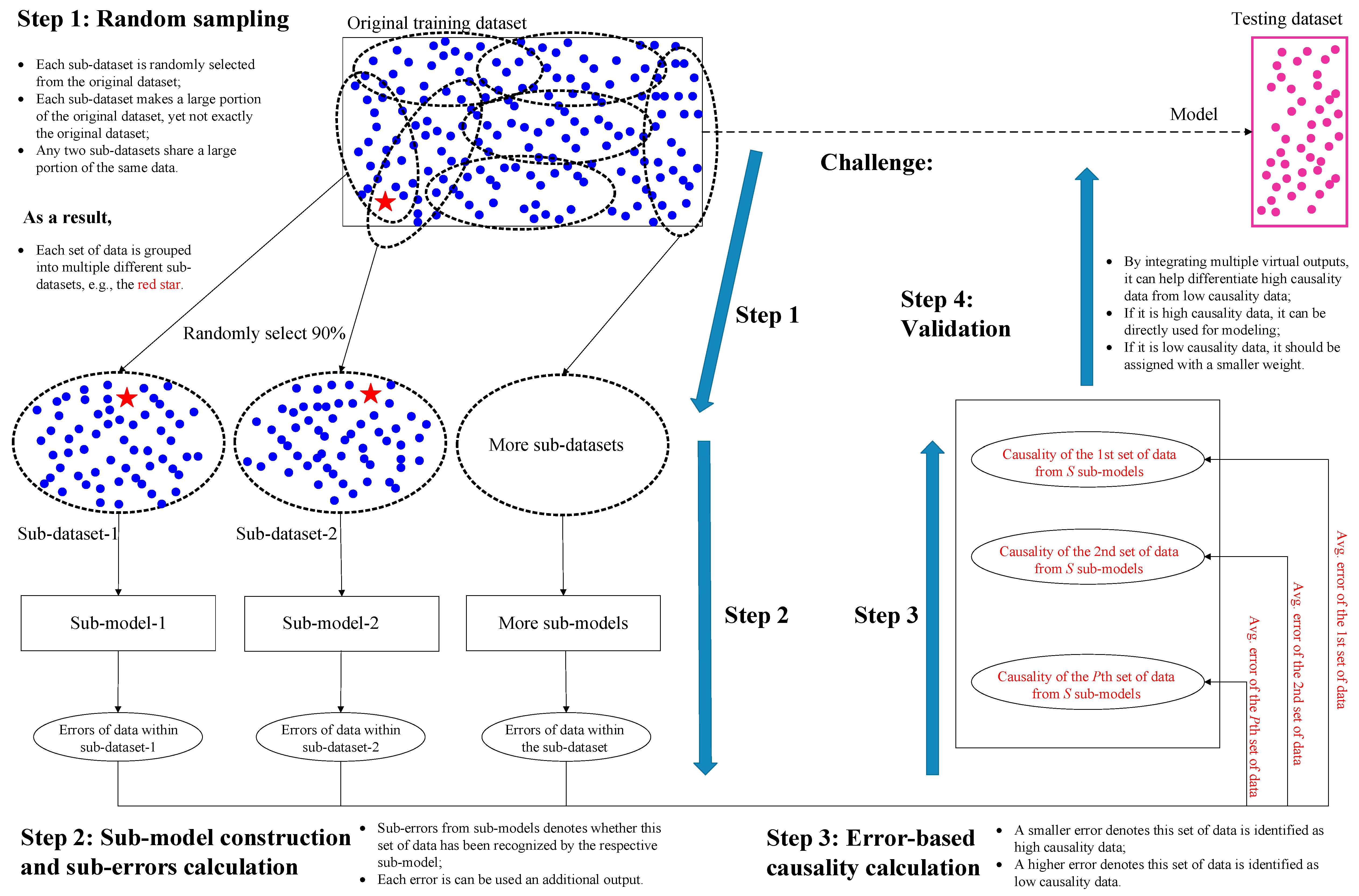
The framework of HiReCau is presented in Figure 1 with four steps.

Figure 1. The framework of the proposed HiReCau method.

Step 1: Random sampling for generating multiple sub-datasets.

Randomly select a large proportion of data from the original training dataset D^T (D for short) to form multiple sub-datasets, D₁, D₂, …, D_s, …, D_S, (see the rectangle in the upper left of Figure 1). More details can be found in Section 2.3.

Step 2: Sub-model construction and sub-error calculation.

Each sub-dataset from Step 1 is used to construct a sub-model using a machine learning approach, Model_s, and the pth set of data can be computed with a sub-error, e_p,s, from the sth sub-model. More details can be found in Section 2.4.

Step 3: Error-based causality calculation.

Calculate the average error e_p,avg using multiple sub-errors from Step 2 as the basis for calculating the data causality δ. Specifically, if δ_p of the pth set of data is relatively high, i.e., e_p,avg is low, it denotes that such data can be recognized by multiple sub-models, and by extension, such data should be recognized as high-causality data; if δ_p of the pth set of data is relatively low, i.e., e_p,avg is high, then such data should be recognized as low-causality. More details can be found in Section 2.5.

Step 4: Validation.

All data can be used to predict the results on the testing dataset D^V by treating high-causality data and low-causality data differently, e.g., data with high δ can be treated equally while data with low δ can be assigned with a much smaller weight. The resilience of HiReCau is also tested. More details can be found in Section 2.6.

2.3. Random Sampling for Generating Multiple Sub-Datasets

Step 1.1: Determine the number and size of sub-datasets.

Normally, it is required that the number of sub-datasets should meet the statistical requirement, i.e., S ≥ 30. For the size φ of the sub-datasets, there is (i) φ (D₁) = φ (D₂) = … = φ (D_s) = … = φ (D_S), and (ii) φ (D₁) = μφ (D^T), μ = 80%, 90%, ….

Step 1.2: Randomly sample data from the original training dataset D_T to construct S sub-datasets.

Determine the sampling method following a certain distribution, e.g., determine the mean μ and variance Δ of normal distribution. Randomly and independently construct S sub-datasets by sampling from the original training dataset D_T for S times.

2.4. Sub-Model Construction and Sub-Error Calculation

Step 2.1: Select a baseline machine learning approach and set the parameters.

Upon exploring the characteristics and requirements of the targeted problem, select a baseline machine learning approach, and determine the relevant parameters. For example, if the data are continuous and there is a relatively large quantity, the neural network (NN) [17,18] is recommended [19]. Then, certain parameters are to be determined, e.g., the number of layers, the number of nodes in each layer, the transfer function, etc.

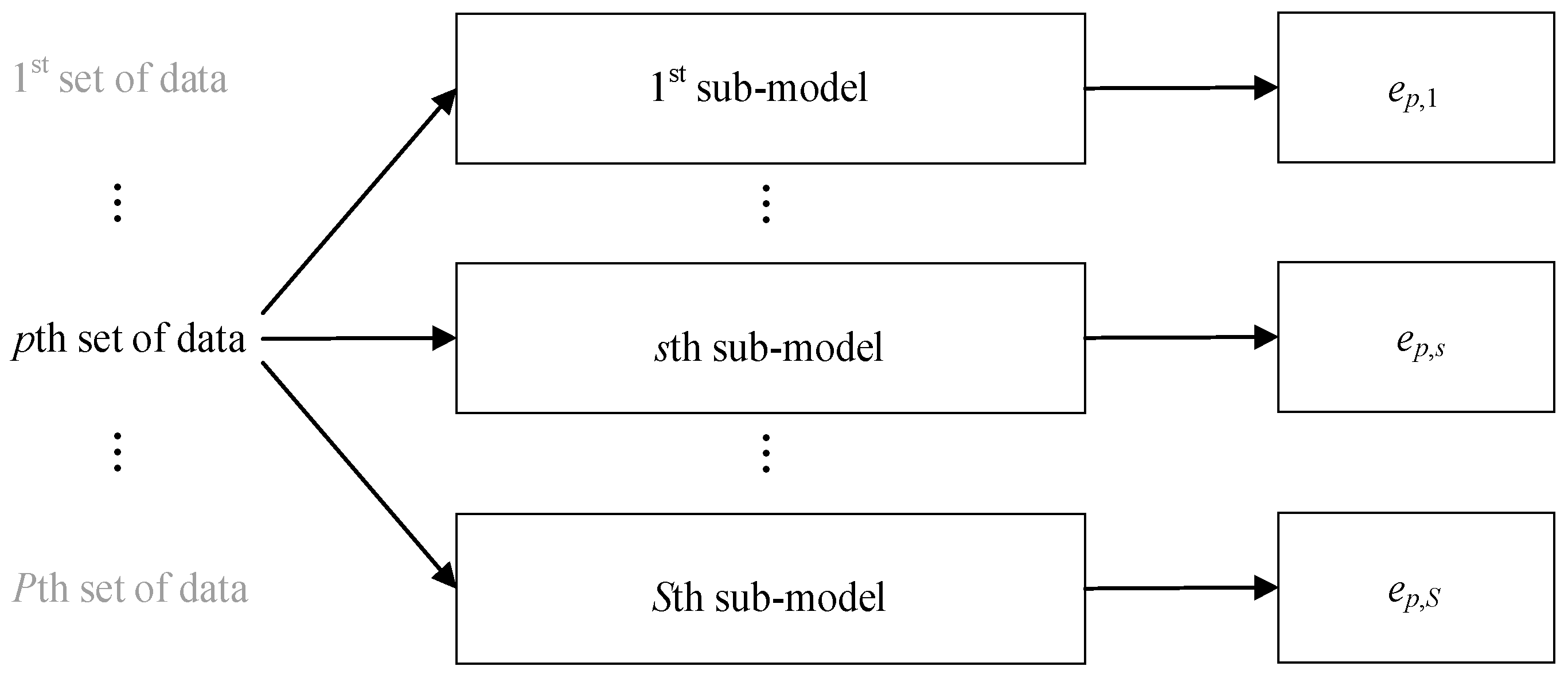
Step 2.2: Construct S sub-models using S sub-datasets and extract the error for the pth set of data from the sth sub-model.

With the selected baseline machine learning approach and its parameters, a total of S sub-models are constructed using S sub-datasets, which is a repeated and independent process. The error of the pth set of data from the sth sub-model is e_p,s, as in Figure 2.

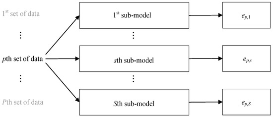
Figure 2. Sub-model construction and error extraction.

2.5. Error-Based Causality Calculation

Step 3.1: Calculate the average error.

For the pth set of data, the average error e_p,avg from S sub-models is calculated by Equation (1),

$$e_{p,avg}=\frac{1}{S}{\displaystyle \sum _{s=1}^S|y_p^a-y_p^s|}$$

(1)

where $y_p^a$ denotes the actual output of the pth set of data and $y_p^s$ denotes the output for the pth set of data from the sth sub-model.

Step 3.2: Calculate the data causality according to the average error.

Since the average error e_p,avg denotes the comprehensive recognition conditions of the pth set of data from S sub-models, the data causality $\epsilon$ is calculated by Equation (2),

$${\epsilon }_p=\underset{p=1,\cdots ,P}{\max }(e_{p,avg})-e_{p,avg}$$

(2)

where $\underset{p=1,\cdots ,P}{\max }(e_{p,avg})$ denotes the maximum of P average errors and each $e_{p,avg}$ is calculated in Step 3.1. There is ${\epsilon }_p\ge 0$ for all $p=1,\cdots ,P$.

2.6. Validation

Step 4.1: Assign weights for the data according to the data causality.

Based on the data causality $\epsilon$, the weight of the pth set of data is determined by Equation (3),

$$w_p=\{\begin{array}{ll}{\alpha }^0=1& \mathrm{if}{\epsilon }_p>{\sigma }_1\\ {\alpha }^1& \mathrm{if}{\sigma }_1\ge {\epsilon }_p>{\sigma }_2\\ ⋮& \\ {\alpha }^n& \mathrm{if}{\sigma }_n\ge {\epsilon }_p\end{array}$$

(3)

where the data causality $\epsilon$ is calculated in Step 3.2, the thresholds $[{\sigma }_1,\cdots {\sigma }_n]$ and the weights parameter $\alpha$ are determined by experts or field engineers.

Step 4.2: Construct a final model with consideration of data weights.

With the same baseline approach in Section 2, the final model is constructed. The objective of the final model can be the mean absolute error (MAE) by Equation (4),

$$MAE=\frac{1}{P}{\displaystyle \sum _{p=1}^P{w}_p*|y_p^a-y_p|}$$

(4)

where w_p is determined in Step 4.1, $y_p^a$ denotes the actual output of the pth set of data, and $y_p$ denotes the output for the pth set of data from the final model.

Step 4.3: Validate the testing dataset.

For the testing dataset with Q sets of data, the mean absolute error (MAE) is calculated by Equation (5) through the constructed final model in Section 4.2.

$$MAE=\frac{1}{Q}{\displaystyle \sum _{q=1}^Q|y_q^a-y_q|}$$

(5)

where $y_q^a$ denotes the actual output of the qth set of testing data and $y_q$ denotes the output for the qth set of testing data from the final model that is constructed in Step 4.2.

Step 4.4: Add additional noise to the training dataset for the resilience test.

Determine two parameters for the resilience test of HiReCau, namely (i) the percentage of noise added to the training dataset, and (ii) the percentage of low-causality data detected by HiReCau, e.g., HiReCau (β%) denotes β% of D_s is detected as low-causality data.

3. Results

3.1. Architecture Design

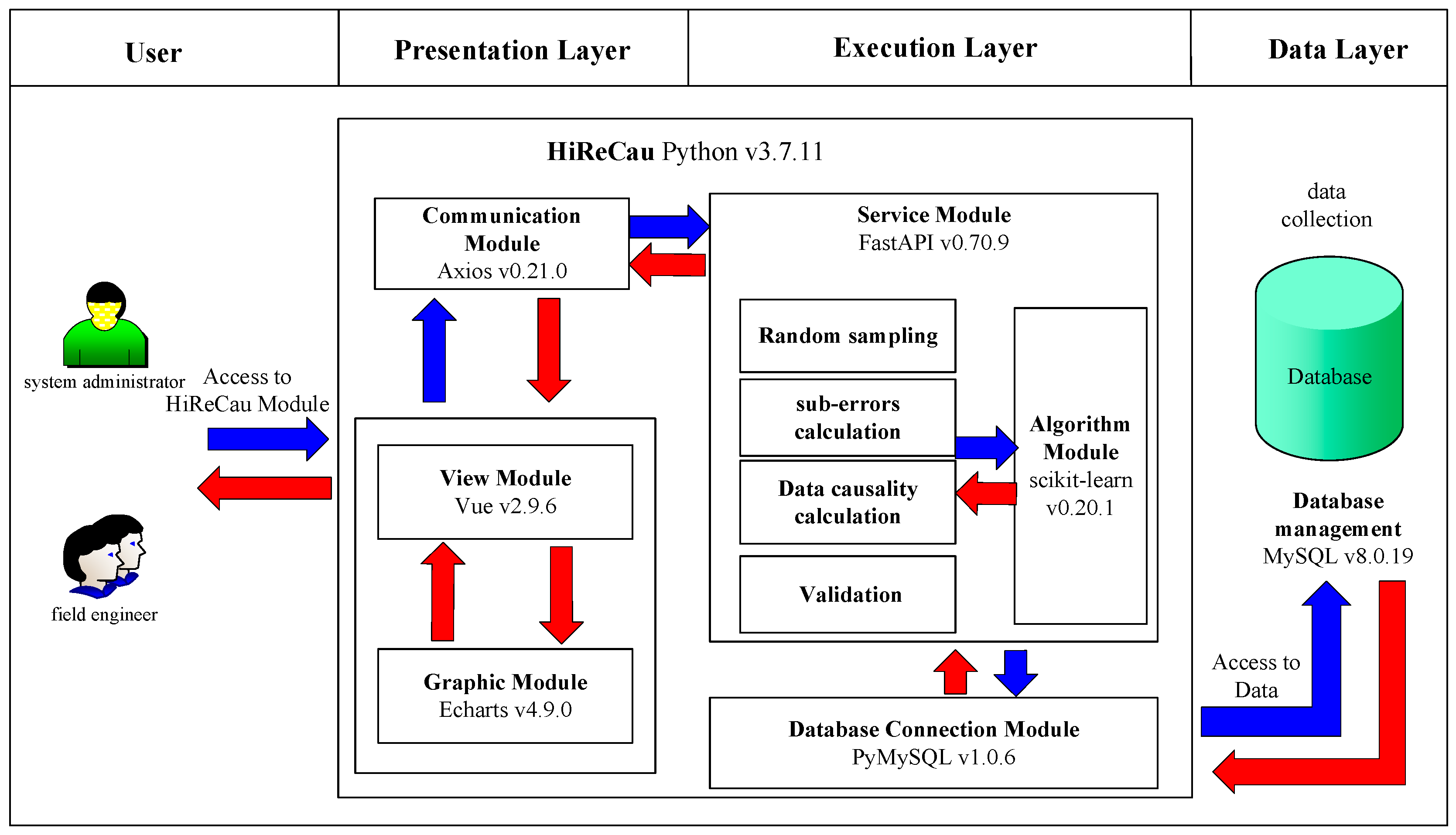
Software is designed and developed, whose architectural design is given in Figure 3. According to Figure 3, there are three layers of software according to the B/S model-based system design and the MVVC (model–view–view model) architecture [20], namely the presentation layer (that includes the View module, the Graphic module, and the Communication module), the execution layer (that includes the Service module, the Algorithm module, and the Database Connection module), and the data layer. The functions of the components of the three layers, as well as the user, are given in Table 2. More details are given in the following subsections.

Figure 3. Software architecture.

Table 2. Compartmentalization of the software.

Module/Role		Functions	What It Interacts with?	Implementation
User		System administrators, field engineers	View module	/
Presentation layer	View module	Interact with users	Receiving requests from Users, and relaying the requests to Graphic module and Communication module	Vue v2.9.6
	Graphic module	Present results	Receiving requests from View module, and providing graphic results	Echarts v4.9.0
	Communication module	Send requests to the service module	View module, and Graphic module	Axios v0.21.0
Execution layer	Service module	Support the Algorithm module	Communication Module, Algorithm module, and Database Connection module	FastAPI 0.70.9
	Algorithm module	Implement the HiReCau method	Service module	scikit-learn v0.20.1
	Database Connection module	Extract and provide data	Service module and the Database	PyMySQL v.1.0.6
Data layer (Database)		Store data Provide access to data	Database Connection module	MySQL v8.0.19

3.2. Presentation Layer Design

• Communication Module by Axios v0.21.0

The Communication module by HiReCau receives the requests from the Graphic module by Vue (fundamentally from the users) and sends the requests to the Service module in the execution layer such as “get”, “post”, etc.

• View module by Vue v2.9.6

The View module of HiReCau is designed as a container to support the Graphic module. The View module is implemented by Vue v2.9.6 which is an incremental framework used for constructing an interface. Vue has the advantage of high extendibility since users can easily build a concise interface. Via the interface constructed by Vue, users can upload data files, and select and input the parameters of the selected baseline machine learning approach, e.g., the number of nodes/layers of the neural network, etc. Then, Vue could (i) load the data files and send the data to Echarts, and (ii) send the loaded data and the selected parameters to the server (i.e., the FastAPI) via the Axios module, and then wait for the response from the server.

• Graphic module by Echarts v4.9.0

The Graphic module of HiReCau is designed to present results for viewing and interacting with the users. It is implemented via Axios which is a powerful and interactive chart with a browser chart and visualization library. Echarts can present data in various forms, e.g., lines, bars, and scattered data, and HiReCau mainly requires lines and scattered data by the original order or ascending order of data causality.

3.3. Execution Layer Design

• Service module by FastAPI 0.70.9

The Service module of HiReCau has two tasks: (i) it receives the requests from the Communication module of the presentation layer and then forwards the requests to the Algorithm module for further calculation, and (ii) it receives the calculation results which are then sent back to the Communication module. FastAPI is used to construct a mini-server to support the web-based Service module since it is a web-based framework with high effectiveness, which can be as effective as NodeJS and Go. Moreover, it is relatively easier to implement, extend, and learn FastAPI.

• Algorithm module by scikit-learn v0.20.1

As a key part of HiReCau, the Algorithm module performs the proposed method, including random sampling, sub-error calculation, data causality calculation, and validation (see Section 2). Concerning the information flow, the Algorithm module performs the requests from the Service module and specifies more search requests, which are then forwarded to the Database Connection module. The Algorithm module is implemented via scikit-learn which is a machine learning base by Python where many machine learning approaches have already been built-in, including the support vector machine (SVM), the random forest (RF), and the neural network (NN). scikit-learn is well known for its convenience and good encapsulation, which can reduce the involvement of human interference while providing multiple interfaces.

• Database Connection module by PyMySQL v.1.0.6

The database connection module of HiReCau is implemented using PyMySQL. Note that MySQL cannot be directly connected to Python. Instead, PyMySQL can be used to connect MySQL with the database. Specifically, PyMySQL receives the data sent from FastAPI and stores the data in MySQL. Then, upon requests from FastAPI, PyMySQL searches related data from the MySQL database and sends the data to FastAPI.

3.4. Data Layer Design

The MySQL module is used in the data layer. MySQL is one of the most prevailing databases owing to its high effectiveness and extendibility [21,22]. Since the HiReCau of this study is WEB-based, MySQL is also one of the most outstanding application software as an RDBMS (relational database management system). Compared with the traditional means that simply store the data in a file, MySQL as a relational database is faster in accessing the data and can be used to store and manage a high volume of data. MySQL is used to permanently store the data for performance enhancement.

4. Case Study

4.1. Case I: A Numerical Case Study and Primary Results

A numerical function is designed for Case I. The function following the normal distribution is given in Equation (6).

$$f(x)=\frac{1}{\sqrt{2\pi }\sigma }\exp \left(-\frac{{\left(x-\mu \right)}^2}{2{\sigma }^2}\right)$$

(6)

where x~N(0, 1) + 1.

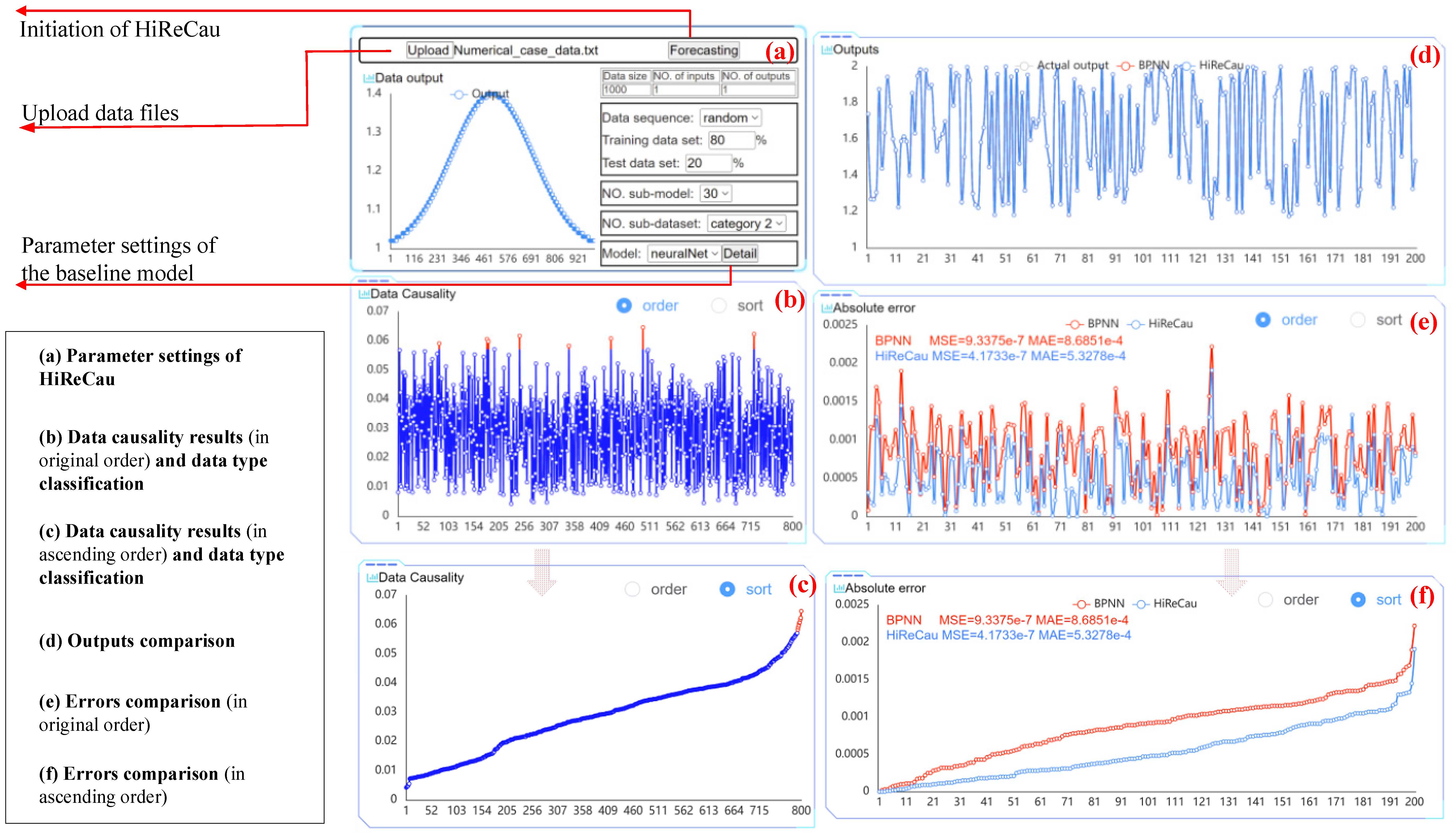
The parameter settings of Case I are given in the following Table 3, and Figure 4 shows the parameter settings part and results of a random run.

Table 3. Parameter settings of Case I.

Steps	Specific Parameter Settings
Overall	A total of 1000 sets of data are randomly generated with 800 sets of data randomly selected as the training dataset and the rest 200 sets of data as the testing dataset, which are set in Figure 4a.
Step 1	With the back-propagation neural network (BPNN) as the baseline approach, its parameter settings are as follows: the number of layers is 4, the number of nodes in the layers is 4, the goal is 0, and the activation function is tanh. Figure 4a shows the section on parameter settings.
Step 2	Two sub-datasets are to be constructed where 1% of the training dataset, i.e., 8 out of 800 sets of data, is identified as low-causality data. Therefore, it is HiReCau (1%) in this case, which is depicted as HiReCau for short in this subsection. The 1% low-causality data and the remaining 99% high-causality data are depicted by the red and green points in Figure 4b,c, respectively.
Step 3	For comparative purposes, the BPNN is also directly used. The parameter settings of the BPNN are the same as in (2). The results are also presented in Figure 4d–f.
Step 4	Users can tune related parameters in (2), tune the proportion of detected low-causality data in (3), or view the results in the original order or the ascending order by data causality or the absolute error depending on their requirements.

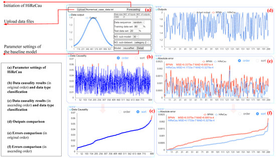
Figure 4. The software interface of Case I.

With the above parameter settings, Figure 4 presents the comparative results of BPNN and HiReCau. According to Figure 4, HiReCau outperforms BPNN in terms of performance. For instance, the mean squared error (MSE) for BPNN stands at 9.3375 × 10⁻⁷, while HiReCau achieves a significantly lower value of 4.1733 × 10⁻⁷. Similarly, the mean absolute error (MAE) for BPNN is 8.6851 × 10⁻⁴, whereas HiReCau demonstrates a lower error of 5.3278 × 10⁻⁴. These improvements represent a significant enhancement of 55.31% in MSE and 38.66% in MAE, thereby highlighting the superiority of HiReCau over BPNN.

4.2. Case I: Resilience Test of Noise Added to the Training Data

This subsection tests the resilience of HiReCau to the added noise to the training dataset. The detailed parameter settings are as follows.

(1)

Percentage of added noise to the training dataset ranges from 10% to 100% at the interval of 10%. The added noise follows from the Pareto distribution (k = 2, xmin = 1).

(2)

The percentage of noise recognized by HiReCau is set as 1%, 1.5%, and 2% denoted by HiReCau (1%), HiReCau (1.5%), and HiReCau (2%), respectively.

(3)

BPNN is used as the baseline approach, and its parameter settings are as follows: nodes in the layers are (10, 10, 10, 10), the transfer function is trainlm, and the goal is 0.

(4)

BPNN is also used for comparative purposes.

(5)

Owing to the randomness brought by training/testing dataset classification and sub-datasets selection, all tests are conducted in 30 runs.

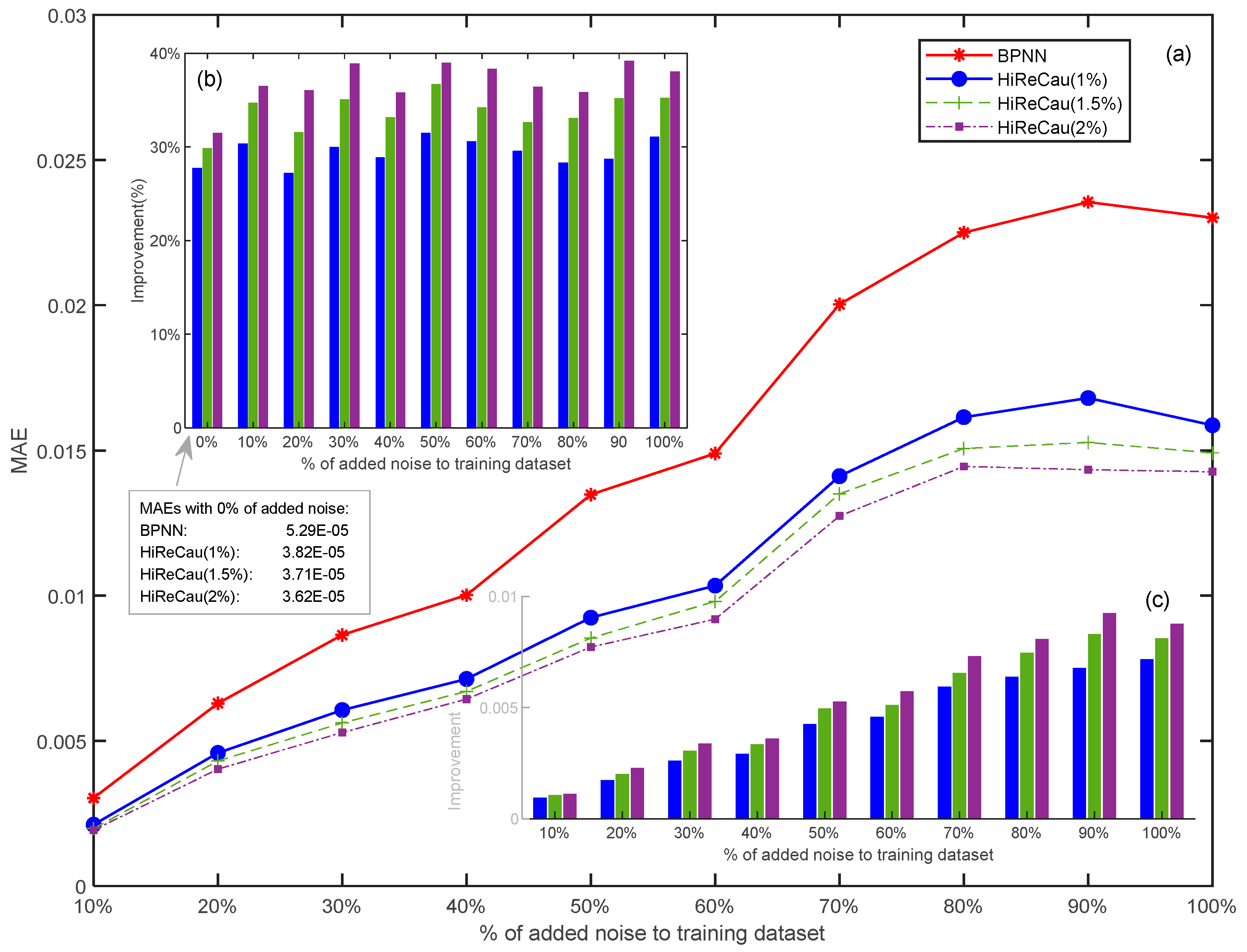
Figure 5 presents the resilience test results

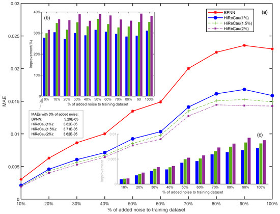
Figure 5. Results of Case I: (a) overall MAE comparison, (b) improvement (%) comparison, and (c) improvement (value) comparison.

According to Figure 5, the following conclusions can be drawn:

(1)

HiReCau demonstrates overall superiority over directly adopting BPNN.

Overall, HiReCau has consistently achieved significantly lower mean absolute errors (MAEs) compared to BPNN in all conditions where there are different percentages of added noise. For instance, in the case of 10% added noisy data, the MAE of HiReCau (1%) stands at 2.1109 × 10⁻³, while BPNN’s MAE is 3.0280 × 10⁻³. As the noise level increases to 100% added noisy data, the MAE of HiReCau (1%) rises to 1.5866 × 10⁻², still notably lower than BPNN’s MAE of 2.3010 × 10⁻². These findings underscore the overall superiority of HiReCau over direct BPNN.

(2)

High resilience when more data are detected by HiReCau as low-causality data (see the continuous and dashed lines in Figure 5).

There is a distinct pattern of performance enhancement, characterized by a decrease in MAEs, as a higher percentage of data is identified as low causality. This trend is visually depicted by the descending dashed line in Figure 5a, the upward slope of the “improvement (%)” graph in Figure 5b, and the increasing “improvement” in Figure 5c. This is partly attributed to the inherent nature of the numerical case, where both the original and noisy data are generated according to fixed Pareto distributions (k = 2, xmin = 1), which guarantees “predictability” within the numerical scenario.

(3)

The stable and consistent superiority of HiReCau over BPNN persists even in the presence of excessive noisy data.

Despite the increasing MAEs observed in both HiReCau and BPNN as more noise is introduced into the training dataset, the comparative advantage of HiReCau over BPNN remains remarkably consistent. Specifically, the overall superiority of HiReCau (1%) hovers around [25%, 30%], while for HiReCau (1.5%) and HiReCau (2%), it stands at [30%, 40%]. Notably, this consistent improvement is evident even in the absence of noise, as seen in the “0%” bars in Figure 5b. It is worth mentioning that although the MAEs of BPNN, HiReCau (1%), HiReCau (1.5%), and HiReCau (2%) are too small to be visually represented in Figure 5a,b, the consistent results remain unchanged.

4.3. Case II: Building Tilt Rate Prediction and Primary Results

During the construction of tunnel systems, the safety of adjacent buildings is inherently vulnerable, necessitating the paramount importance of real-time monitoring of building tilt rate (BTR). Neglecting BTR can lead to dire consequences, including structural instability, potential collapse, and damage to adjacent properties [1]. Moreover, BTR is influenced by various factors such as soil movement, groundwater levels, and the dynamics of excavation works [2]. Therefore, vigilant monitoring and prompt mitigation measures (which, however, are beyond the scope of this study) can significantly reduce the risks associated with tunnel construction and protect the integrity of the surrounding buildings.

The practical case is to predict the building tilt rate (BTR) of Metro Line No. 6 in the city of Wuhan, China [3,7]. The parameter settings of Case II are given in the following Table 4.

Table 4. Parameter settings of Case II.

Steps	Specific Parameter Settings
Overall	A total of 500 sets of data have been collected with sixteen attributes in the input, namely the building factors, e.g., the distance to the construction site, etc., the tunnel-related factors, e.g., the soil type, etc., and the tunnel boring machine (TBM) factors, e.g., the torque of TBM, and the BTR as the output. Among 500 sets of data, the first 400 sets of data are used as the training dataset and the remaining 100 as the testing dataset.
Steps	With BPNN still the baseline approach, its parameter settings are as follows: the number of layers is 4, the number of nodes in the layers is 10, the goal is 1 × 10−4, and the activation function is logistic.

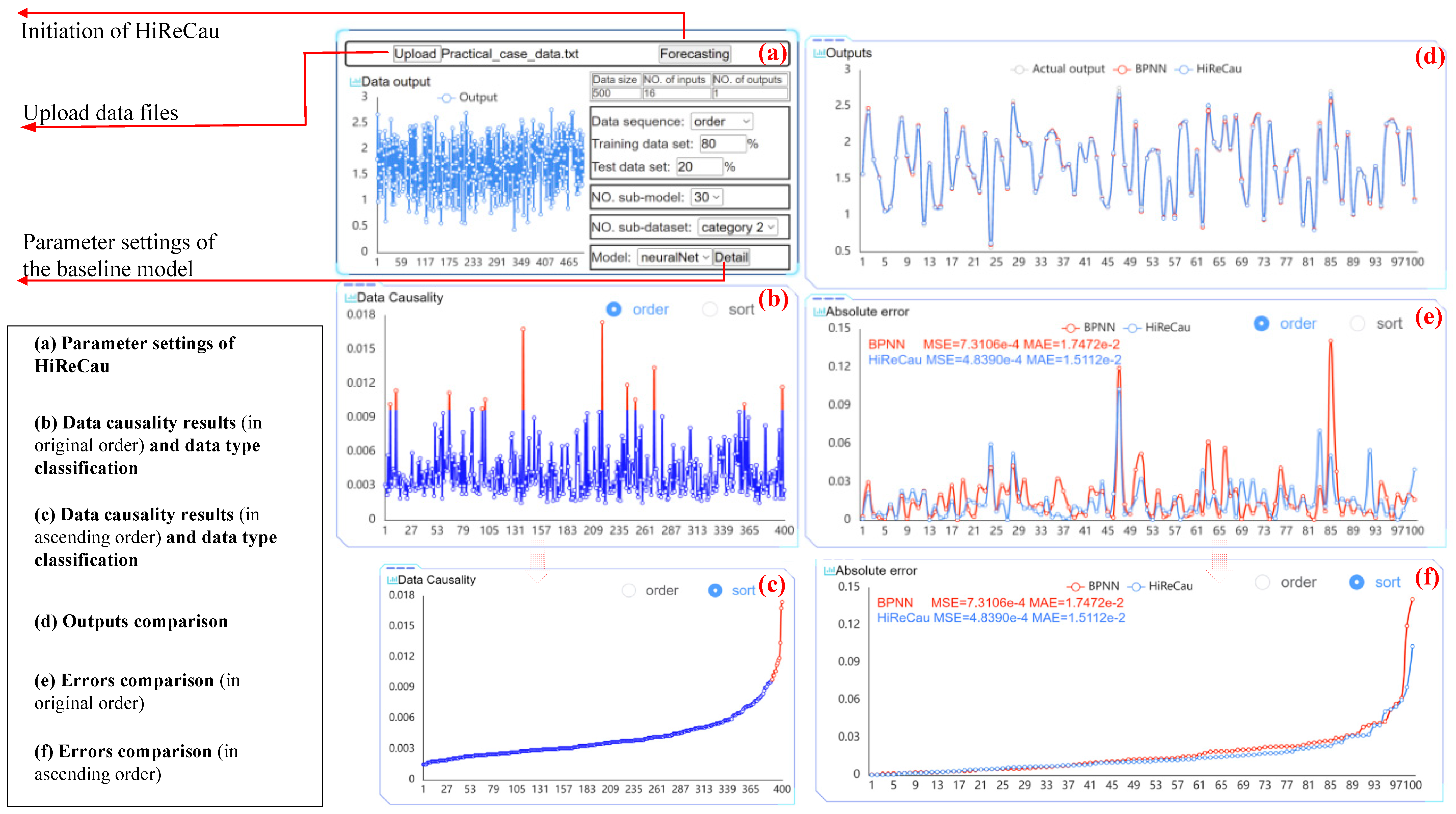
Figure 6 shows the parameter settings part and results of a random run. As depicted in Figure 6b,c, the data causality calculation results indicate that 3% of the 400 data points were identified as low-causality data, representing the HiReCau (3%) approach. Figure 6d compares the outputs, while Figure 6e,f present a comparative analysis of the errors. Based on the data presented in Figure 6, it is evident that HiReCau generally outperforms the direct application of BPNN. For instance, the mean squared error (MSE) is reduced from 7.3106 × 10⁻⁴ with BPNN to 4.8390 × 10⁻⁴ with HiReCau, representing a 33.81% improvement. Similarly, the mean absolute error (MAE) decreases from 1.7472 × 10⁻² with BPNN to 1.5112 × 10⁻² with HiReCau, yielding a 13.51% improvement.

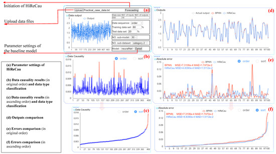
Figure 6. The software interface of Case II.

4.4. Case II: Resilience Test of Noise Added to the Training Data

Further resilience tests are conducted with the following parameter settings.

(1)

In total, 5–50% of additional noisy data are considered in the training dataset which is randomly selected from a total of 400 sets of original data.

(2)

The remaining 100 sets of original data are used as the testing dataset to be consistent with previous researchers.

(3)

In total, 10% of the training data are recognized as noisy data by HiReCau with the results of 5% as noisy data presented above.

(4)

BPNN is still used as the baseline approach with the same parameter settings (see Section 4.3).

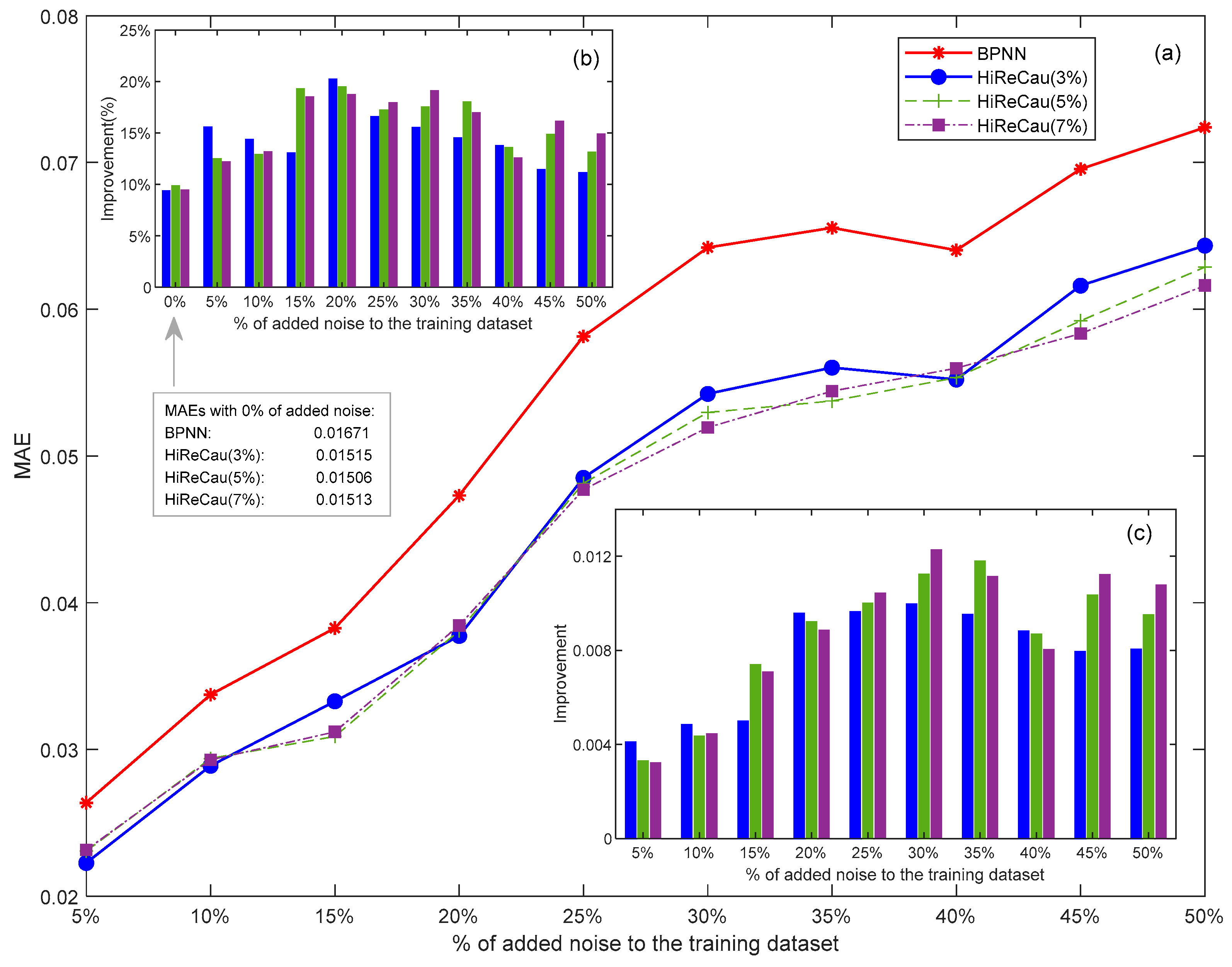
With the above parameter settings, the resilience test of Case II is given in Figure 7.

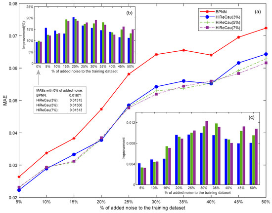
Figure 7. Results of Case II: (a) overall MAE comparison, (b) improvement (%) comparison, and (c) improvement (value) comparison.

According to Figure 7, the following conclusions can be drawn:

(1)

HiReCau demonstrates overall superiority over directly adopting BPNN.

Overall, HiReCau demonstrates superior performance over direct BPNN, achieving significantly smaller MAEs across all conditions with varying percentages of added noise. For instance, when 5% noisy data are added, the MAE of HiReCau (3%) is 2.2259 × 10⁻², which is notably lower than the 2.6362 × 10⁻² MAE of BPNN. Similarly, as the noise level increases to 50%, the MAE of HiReCau (3%) rises to 6.4335 × 10⁻², still outperforming the MAE of 7.2384 × 10⁻² by directly adopting BPNN.

(2)

A first increase then decrease in improvement is observed when a greater amount of noisy data is introduced to the training dataset.

As depicted in Figure 7b,c, two notable trends can be observed: (i) an upward trend in both the percentage (Figure 7b) and values (Figure 7c) of improvement as the percentage of added noise increases from 5% to approximately 20–30%, and (ii) a subsequent decreasing trend in improvement when the amount of noisy data exceeds 30% of the training dataset. This first-increasing-then-decreasing improvement is evident in the case of HiReCau at 3%. This pattern is likely attributed to the inherent complexity of the BTR data, particularly when contrasted with the results from numerical cases where all data are artificially generated according to a fixed Pareto distribution (k = 2, xmin = 1).

(3)

Intertwined MAEs are presented when different percentages of low-causality data are identified by HiReCau (see the continuous and dashed lines in Figure 7).

Initially, when there is less noisy data, detecting a lower percentage of low-causality data using HiReCau leads to slightly better performance. For instance, HiReCau (3%) detecting 3% low-causality data outperforms HiReCau (5%) and HiReCau (7%) when 5%-10% noisy data are introduced. Conversely, when there is more noisy data, detecting a greater amount of low-causality data using HiReCau yields less prominent superior results. For example, HiReCau (7%) produces better outcomes than HiReCau (5%) and HiReCau (3%) when 45–50% noisy data is added. Overall, the variations in performance between HiReCau detecting different percentages of low-causality data are not significant, particularly when compared to the numerical case (Section 4.3). This could also be attributed to the inherent randomness in the BTR data and by extension most practical scenarios in a generic sense.

5. Conclusions

A new HiReCau method is proposed for high resilient asymmetry detection for abnormal building tilt rate detection.

The advantages and theoretical contributions of this study are as follows.

(1)

Different from traditional studies that treat all data equally, the data causality reflects the input–output relation of data and it is used to update the weight of data that are used to construct the final model.

(2)

HiRECau is equipped with the high (Hi) resilience (Re) ability to detect both the existent and added noise in the training dataset owing to detecting the data causality (Cau).

(3)

Last but not least, this study gives specifics concerning the implementation of HiReCau, including software development and case parameter settings, which are highly beneficial for researchers and practitioners in varied fields.

One numerical case and another practical case are studied in this paper for validation, which show highly consistent results.

(1)

HiReCau outperforms only adopting BPNN under different levels of additional noisy data to the training dataset, which indicates the high resilience of HiReCau. Specifically, for the BTR detection case, it is found that HiReCau can reduce the MSE and MAE by 33.81% and 13.51% compared with BPNN.

(2)

This superiority is maintained when a higher percentage of low-causality data is detected by HiReCau. Specifically, for the BTR detection case, a first-increasing-then-decreasing improvement of HiReCau over BPNN is found. All in all, the two cases have sufficiently validated the effectiveness and resilience of the proposed HiReCau method.

The limitations of this study are as follows.

(1)

Only one output, i.e., the BTR is considered in this study, which is restricted by the theoretical requirement that BPNN can only handle problems with a single output.

(2)

Only BPNN is tested as the baseline model in this study, whereas HiReCau is proposed as model-independent.

(3)

The data size in this study is relatively small, which should be expanded for a more comprehensive test.

For future studies, the proposed HiReCau approach could be tested by handling multiple outputs, e.g., daily and accumulated settlements included. Moreover, other theoretical and practical cases should also be tested to provide a more holistic understanding of HiReCau. Finally, the new concept of noisy data based on data causality should be further explored to further its theoretical foundations.

References

- Zhang, L.; Wu, X.; Zhu, H.; AbouRizk, S.M. Perceiving safety risk of buildings adjacent to tunneling excavation: An information fusion approach. Autom. Constr. 2017, 73, 88–101. [Google Scholar] [CrossRef]
- Franza, A.; Marshall, A.M. Centrifuge and real-time hybrid testing of tunneling beneath piles and piled buildings. J. Geotech. Geoenviron. Eng. 2019, 145, 04018110. [Google Scholar] [CrossRef]
- Simsion, G.; Witt, G. Data Modeling Essentials; Morgan Kaufmann: San Francisco, CA, USA, 2004. [Google Scholar]
- Chang, L.L.; Fu, C.; Wu, Z.J.; Liu, W.Y. A Data-Driven Method Using BRB With Data Reliability and Expert Knowledge for Complex Systems Modeling. IEEE Trans. Syst. Man. Cybern Syst. 2021, 52, 6729–6743. [Google Scholar] [CrossRef]
- Chang, L.L.; Zhang, L.M.; Fu, C.; Chen, Y.W. Transparent digital twin for output control using belief rule base. IEEE Trans. Cybern. 2021, 52, 10364–10378. [Google Scholar] [CrossRef] [PubMed]
- Park, H.Y.; Kim, K.J. Sentiment analysis of movie review using integrated CNN-LSTM model. J. Intell. Inf. Syst. 2019, 25, 141–154. [Google Scholar]
- Yang, H.; Song, K.; Zhou, J. Automated Recognition Model of Geomechanical Information Based on Operational Data of Tunneling Boring Machines. Rock. Mech. Rock. Eng. 2022, 55, 1499–1516. [Google Scholar] [CrossRef]
- Zhu, W.; Chang, L.L.; Sun, J.B.; Wu, G.H.; Xu, X.B.; Xu, X.J. Parallel multipopulation optimization for belief rule base learning. Inf. Sci. 2021, 556, 436–458. [Google Scholar] [CrossRef]
- Li, R.; Wen, Q.Q.; Tan, W.C.; Zhang, Y.J. Adaptive weighting impact angle optimal guidance law considering seeker’s FOV angle constraints. J. Syst. Eng. Electron. 2018, 29, 142–151. [Google Scholar] [CrossRef]
- Wang, D.; Liu, K.; Zhang, X. A Generic Indirect Deep Learning Approach for Multisensor Degradation Modeling. IEEE Trans. Autom. Sci. Eng. 2021, 19, 1924–1940. [Google Scholar] [CrossRef]
- Sourati, J.; Evans, J.A. Accelerating science with human-aware artificial intelligence. Nat. Human. Behav. 2023, 7, 1682–1696. [Google Scholar] [CrossRef] [PubMed]
- Hu, J.; Zhang, H.; Liu, H.; Yu, X. A survey on sliding mode control for networked control systems. Int. J. Syst. Sci. 2021, 52, 1129–1147. [Google Scholar] [CrossRef]
- Wazid, M.; Das, A.K.; Hussain, R.; Succi, G.; Rodrigues, J.J. Authentication in cloud-driven IoT-based big data environment: Survey and outlook. J. Syst. Archit. 2019, 97, 185–196. [Google Scholar] [CrossRef]
- Xu, X.L.; Chen, W.; Sun, Y.F. Over-sampling algorithm for imbalanced data classification. J. Syst. Eng. Electron. 2019, 30, 1182–1191. [Google Scholar] [CrossRef]
- Zhou, C.; Ding, L.; Zhou, Y.; Skibniewski, M.J. Visibility graph analysis on time series of shield tunneling parameters based on complex network theory. Tunn. Undergr. Space Technol. 2019, 89, 10–24. [Google Scholar] [CrossRef]
- Brunton, S.L.; Kutz, J.N. Data-Driven Science and Engineering Machine Learning, Dynamical Systems, and Control; Cambridge University Press: Cambridge, UK, 2022. [Google Scholar]
- Liu, D.; Ding, W.; Dong, Z.S.; Pedrycz, W. Optimizing deep neural networks to predict the effect of social distancing on COVID-19 spread. Comput. Ind. Eng. 2022, 166, 107970. [Google Scholar] [CrossRef] [PubMed]
- Mumali, F. Artificial neural network-based decision support systems in manufacturing processes: A systematic literature review. Comput. Ind. Eng. 2022, 165, 107964. [Google Scholar] [CrossRef]
- Bhalke, D.G.; Rao, C.B.; Bormane, D.S. Automatic musical instrument classification using fractional fourier transform based-MFCC features and counter propagation neural network. J. Intell. Inf. Syst. 2016, 46, 425–446. [Google Scholar] [CrossRef]
- Kouraklis, J. MVVM as Design Pattern. In MVVM in Delphi; Apress: Berkeley, CA, USA, 2016; pp. 1–12. [Google Scholar]
- Gabryel, M. The bag-of-features algorithm for practical apps using MySQL. In International Conference on Soft Computing; Springer: Cham, Switzerland, 2016; pp. 635–646. [Google Scholar]
- Krogh, J.W.; Krogh, G. ; Gennick. MySQL Connector/Python Revealed; Apress: New York, NY, USA, 2018. [Google Scholar]
Disclaimer/Publisher’s Note: The statements, opinions and data contained in all publications are solely those of the individual author(s) and contributor(s) and not of MDPI and/or the editor(s). MDPI and/or the editor(s) disclaim responsibility for any injury to people or property resulting from any ideas, methods, instructions or products referred to in the content. |
© 2024 by the authors. Licensee MDPI, Basel, Switzerland. This article is an open access article distributed under the terms and conditions of the Creative Commons Attribution (CC BY) license (https://creativecommons.org/licenses/by/4.0/).