Dynamics of a Stochastic Vector-Borne Model with Plant Virus Disease Resistance and Nonlinear Incidence

Abstract

Symmetry in mathematical models often refers to invariance under certain transformations. In stochastic models, symmetry considerations must also account for the probabilistic nature of inter- actions and events. In this paper, a stochastic vector-borne model with plant virus disease resistance and nonlinear incidence is investigated. By constructing suitable stochastic Lyapunov functions, we show that if the related threshold $R_0^s<1$, then the disease will be extinct. By using the reproduction number $R_0$, we establish sufficient conditions for the existence of ergodic stationary distribution to the stochastic model. Furthermore, we explore the results graphically in numerical section and find that random fluctuations introduced in the stochastic model can suppress the spread of the disease, except for increasing plant virus disease resistance and decreasing the contact rate between infected plants and susceptible vectors. The results reveal the correlation between symmetry and stochastic vector-borne models and can provide deeper insights into the dynamics of disease spread and control, potentially leading to more effective and efficient management strategies.

1. Introduction

Diseases caused by plant viruses seriously impede the yield and quality of crops all over the world [1]. Almost 1100 species of plant viruses have been reported [2], among which, for instance, tomato spotted wilt virus (TSWV) is one of the deadliest, with a host range of more than 1000 plants species belonging to more than 85 families including tomato, bean, lettuce, groundnut, pepper, potato, and tobacco [3,4,5,6]. TSWV is spread by at least eight different species of thrips, with the western flower thrip (WFT) identified as the primary vector responsible for its extensive distribution [7,8]. The virus-carrying WFT was first detected in the western United States and rapidly spread to other countries via international trade.

In recent years, more and more mathematical models have been established to study plant diseases, and many researchers have been interested in the influence of host demography, the weather, temperature, seasonal variations, and so on; see, e.g., [9,10,11,12,13,14,15]. Over extended periods of interaction, plants have developed intricate defense mechanisms, known as disease resistance, through mutual adaptation, selection, and even co-evolution with pathogens [1]. For example, five distinct genes responsible for TSWV resistance in tomatoes have been identified in studies [16,17].

In 2020, Fei, Zou and Chen [1] investigated the following vector-borne model with plant disease resistance and nonlinear incidence:

$$\left\{\begin{array}{c}{\displaystyle \frac{dS}{dt}}=\mu K+cE+(b+d)I-\mu S-\left({\displaystyle \frac{{\beta }_{vh}Y}{1+{\alpha }_{vh}Y}}+{\displaystyle \frac{{\beta }_{hh}I}{1+{\alpha }_{hh}I}}\right)S,\hfill \\ {\displaystyle \frac{dE}{dt}}=\left({\displaystyle \frac{{\beta }_{vh}Y}{1+{\alpha }_{vh}Y}}+{\displaystyle \frac{{\beta }_{hh}I}{1+{\alpha }_{hh}I}}\right)S-(c+ϵ+\mu )E,\hfill \\ {\displaystyle \frac{dI}{dt}}=ϵE-(b+\mu +\gamma +d)I,\hfill \\ {\displaystyle \frac{dR}{dt}}=\gamma I-\mu R,\hfill \\ {\displaystyle \frac{dX}{dt}}=\Lambda -{\beta }_{hv}XI-mX,\hfill \\ {\displaystyle \frac{dY}{dt}}={\beta }_{hv}XI-mY.\hfill \end{array}\right.$$

(1)

where all the parameters in model (1) are nonnegative constants, and $S,E,I,R,X$, and Y represent the number of susceptible individuals, exposed individuals, infectious individuals, recovered individuals, and the densities of the susceptible vectors and infected vectors at time t, respectively. For the biological interpretations of the other parameters, see Table 1 in [1]. They showed that the basic reproduction number of model (1) is

$$R_0={\displaystyle \frac{Kϵ(m^2{\beta }_{hh}+{\beta }_{hv}{\beta }_{vh}\Lambda )}{m^2(c+ϵ+\mu )(b+\mu +\gamma +d)}}.$$

(2)

It is proved that if $R_0<1$, the disease-free equilibrium is globally asymptotically stable, and if $R_0>1$ and $\mu >max\left({\displaystyle \frac{2{\beta }_{vh}K\Lambda }{m\rho {(1+{\alpha }_{vh}\rho )}^2}},{\displaystyle \frac{2{\beta }_{hh}K}{{(1+{\alpha }_{hh}\rho )}^2}}-2(b+d)-\gamma \right)$ as defined in Theorem 4.2. in [1], model (1) has an endemic equilibrium $(S^{*},E^{*},I^{*},R^{*},X^{*},Y^{*})$ which is globally asymptotically stable.

From the perspective of mathematical biology, stochastic epidemic models are crucial because they account for randomness and variability in disease transmission, which are often present in real-world scenarios. This allows for more accurate predictions and an understanding of disease dynamics, particularly in small populations or under fluctuating environmental conditions, where deterministic models may fall short. Recent progress in stochastic differential equations has enabled the incorporation of randomness into the analysis of such phenomena, such as introducing random noise into the differential equation system or accounting for environmental fluctuations in parameter values; see, e.g., [18,19,20,21,22,23,24,25,26,27,28,29,30,31,32].

Motivated by the above works, we shall focus on the following stochastic vector-borne model with plant virus disease resistance and nonlinear incidence:

$$\left\{\begin{array}{c}dS=\left(\mu K+cE+(b+d)I-\mu S-\left({\displaystyle \frac{{\beta }_{vh}Y}{1+{\alpha }_{vh}Y}}+{\displaystyle \frac{{\beta }_{hh}I}{1+{\alpha }_{hh}I}}\right)S\right)dt+{\sigma }_{1}Sd{B}_1\left(t\right),\hfill \\ dE=\left(\left({\displaystyle \frac{{\beta }_{vh}Y}{1+{\alpha }_{vh}Y}}+{\displaystyle \frac{{\beta }_{hh}I}{1+{\alpha }_{hh}I}}\right)S-(c+ϵ+\mu )E\right)dt+{\sigma }_{2}Ed{B}_2\left(t\right),\hfill \\ dI=\left(ϵE-(b+\mu +\gamma +d)I\right)dt+{\sigma }_{3}Id{B}_3\left(t\right),\hfill \\ dR=\left(\gamma I-\mu R\right)dt+{\sigma }_{4}Rd{B}_4\left(t\right),\hfill \\ dX=\left(\Lambda -{\beta }_{hv}XI-mX\right)dt+{\sigma }_{5}d{B}_5\left(t\right),\hfill \\ dY=\left({\beta }_{hv}XI-mY\right)dt+{\sigma }_{6}d{B}_6\left(t\right),\hfill \end{array}\right.$$

(3)

where $B_i\left(t\right)$ $(i=1,2,\dots ,6)$ are independent standard Brownian motions with $B_i\left(0\right)=0$ and ${\sigma }_i^2>0$ denoting the intensities of white noise.

In the context of epidemiological models, symmetry can mean spatial symmetry, temporal symmetry, and parameter symmetry. In stochastic models, symmetry considerations must also account for the probabilistic nature of interactions and events. This involves looking at the statistical symmetries or invariance in the distribution of states or events over time and space. In the field of studying the dynamic behavior of the epidemic model, one of the most important parts is to analyze steady states together with their stability [31,33]. This problem can be solved by the stability of the disease-free equilibrium (endemic equilibrium) through the basic reproduction number $R_0$ of the deterministic model [1]. However, for stochastic model (3), there is no endemic equilibrium. Khasminskii [34] showed that the existence of an ergodic stationary distribution to model (3) can reveal the persistence of the infection.

In this paper, we investigate the extinction and the existence of ergodic stationary distribution for model (3). With the help of Lyapunov function, we establish sufficient conditions for the extinction and the existence of ergodic stationary distribution. Moreover, we explore some numerical simulations to support our results.

We organize this paper as follows. In Section 2, we present some preliminaries. In Section 3, we establish sufficient conditions for the extinction and the existence of ergodic stationary distribution of model (3). In Section 4, we provide some numerical simulations to support our results. Finally, we end our work with some concluding remarks.

2. Preliminaries

Before discussing the long term behavior of system (3), we first consider the existence and uniqueness of the global positive solution.

Lemma 1.

For any initial value $X\left(0\right)=(S\left(0\right),E\left(0\right),I\left(0\right),R\left(0\right),X\left(0\right),Y\left(0\right))\in {\mathbb{R}}_{+}^6$, there is a unique solution $X\left(t\right)=\left(S\right(t),E(t),I(t),R(t),X(t),Y(t\left)\right)$ of system (3) on $t\ge 0$ and the solution will remain in ${\mathbb{R}}_{+}^6$ with probability one.

Proof. 

As the coefficients of system (3) satisfy the local Lipschitz condition, there is a unique local solution on [0,${\tau }_e$) for any initial value $X\left(0\right)\in {\mathbb{R}}_{+}^6$, where ${\tau }_e$ is the explosion time [26]. In order to show the globality of this solution, we need to prove that ${\tau }_e=\infty$ almost surely (briefly a.s.). Let $k_0$ be sufficiently large such that $X_0$ lies in the interval ${[{\displaystyle \frac{1}{k_0}},k_0]}^6$. For each integer $k>k_0$, define the stopping time as follows

$${\tau }_k=inf\left\{t\in [0,{\tau }_e):minV\left(t\right)\le {\displaystyle \frac{1}{k}}ormaxV\left(t\right)\ge k\right\},$$

Set $inf\varnothing =\infty$ (∅ denotes the empty set). It is easy to see that ${\tau }_k$ is increasing as $k\to \infty$. Set ${\tau }_{\infty }=\underset{k\to \infty }{lim}{\tau }_k$, then ${\tau }_{\infty }\le {\tau }_e$ a.s. If we can show that ${\tau }_{\infty }=\infty$ a.s. then ${\tau }_e=\infty$ and $X\left(t\right)\in {\mathbb{R}}_{+}^6$ a.s. for all $t\ge 0$. In other words, to complete the proof, all we need to show is that ${\tau }_{\infty }=\infty$ a.s. If this assertion is violated, there exists a constant $T>0$ and $\eta \in (0,1)$ such that $P\{{\tau }_{\infty }\le T\}>\eta$. Consequently, there is an integer $k_1\ge k_0$ such that $P\{{\tau }_k\le T\}>\eta$ for all $k\ge k_1$.

Define a $C^2-function$ W: ${\mathbb{R}}_{+}^6\to {\mathbb{R}}_{+}^1$

$$\begin{array}{cc}\hfill W(S,E,I,R,X,Y)=& (S-1-lnS)+(E-1-lnE)+(I-1-lnI)+(R-1-lnR)\\ & +(X-a-aln{\displaystyle \frac{X}{a}})+(Y-1-lnY).\end{array}$$

The non-negativity of this function can be obtained from $u-1-lnu\ge 0foranyu>0.$

By It$\widehat{o}$’s formula, we have

$$\begin{array}{cc}\hfill dW(S,E,I,R,X,Y)=& LWdt+{\sigma }_1(S-1)d{B}_1\left(t\right)+{\sigma }_2(E-1)d{B}_2\left(t\right)+{\sigma }_3(I-1)d{B}_3\left(t\right)\hfill \\ & +{\sigma }_4(R-1)d{B}_4\left(t\right)+{\sigma }_5(X-1)d{B}_5\left(t\right)+{\sigma }_6(Y-1)d{B}_6\left(t\right),\hfill \end{array}$$

where

$$\begin{array}{cc}\hfill LW=& \left(1-{\displaystyle \frac{1}{S}}\right)\left(\mu K+cE+(b+d)I-\mu S-\left({\displaystyle \frac{{\beta }_{vh}Y}{1+{\alpha }_{vh}Y}}+{\displaystyle \frac{{\beta }_{hh}I}{1+{\alpha }_{hh}I}}\right)S\right)\hfill \\ & +\left(1-{\displaystyle \frac{1}{E}}\right)\left(\left({\displaystyle \frac{{\beta }_{vh}Y}{1+{\alpha }_{vh}Y}}+{\displaystyle \frac{{\beta }_{hh}I}{1+{\alpha }_{hh}I}}\right)S-(c+ϵ+\mu )E\right)+\left(1-{\displaystyle \frac{1}{I}}\right)\left(ϵE-(b+\mu +\gamma +d)I\right)\hfill \\ & +\left(1-{\displaystyle \frac{1}{R}}\right)(\gamma I-\mu R)+\left(1-{\displaystyle \frac{1}{X}}\right)\left(\Lambda -{\beta }_{hv}XI-mX\right)+\left(1-{\displaystyle \frac{1}{Y}}\right)\left({\beta }_{hv}XI-mY\right)\hfill \\ & +{\displaystyle \frac{1}{2}}({\sigma }_1^2+{\sigma }_2^2+{\sigma }_3^2+{\sigma }_4^2+{\sigma }_5^2+{\sigma }_6^2)\hfill \\ \hfill \le & \mu (K-S-E-I-R)+\Lambda -m(X+Y)+{\displaystyle \frac{{\beta }_{vh}Y}{1+{\alpha }_{vh}Y}}+{\displaystyle \frac{{\beta }_{hh}I}{1+{\alpha }_{hh}I}}+a{\beta }_{hv}I+4\mu +c+ϵ\hfill \\ & +b+d+\gamma +m+am+{\displaystyle \frac{1}{2}}({\sigma }_1^2+{\sigma }_2^2+{\sigma }_3^2+{\sigma }_4^2+{\sigma }_5^2+{\sigma }_6^2).\hfill \end{array}$$

We define $a={\displaystyle \frac{\mu }{{\beta }_{hv}}}$. And then, we can obtain

$$\begin{array}{cc}\hfill LW\le & \mu (K-S-E-R)+\Lambda -m(X+Y)+{\displaystyle \frac{{\beta }_{vh}Y}{1+{\alpha }_{vh}Y}}+{\displaystyle \frac{{\beta }_{hh}I}{1+{\alpha }_{hh}I}}+4\mu +c+ϵ\hfill \\ \hfill & +b+d+\gamma +m+am+{\displaystyle \frac{1}{2}}({\sigma }_1^2+{\sigma }_2^2+{\sigma }_3^2+{\sigma }_4^2+{\sigma }_5^2+{\sigma }_6^2)\hfill \\ \hfill \le & \mu K+\Lambda +4\mu +c+ϵ+b+d+\gamma +m+{\displaystyle \frac{\mu m}{{\beta }_{hv}}}+{\displaystyle \frac{{\beta }_{vh}}{{\alpha }_{vh}}}+{\displaystyle \frac{{\beta }_{hh}}{{\alpha }_{hh}}}+{\displaystyle \frac{1}{2}}({\sigma }_1^2+{\sigma }_2^2+{\sigma }_3^2+{\sigma }_4^2+{\sigma }_5^2+{\sigma }_6^2)\hfill \\ \hfill \doteq & F.\hfill \end{array}$$

Hence, there exists a suitable positive constant F independent of $S\left(t\right)$, $E\left(t\right)$, $I\left(t\right)$, $R\left(t\right)$, $X\left(t\right)$, $Y\left(t\right)$, and t. So we have

$$\begin{array}{cc}\hfill dW\le & Fdt+{\sigma }_1(S-1)d{B}_1\left(t\right)+{\sigma }_2(E-1)d{B}_2\left(t\right)+{\sigma }_3(I-1)d{B}_3\left(t\right)\hfill \\ \hfill & +{\sigma }_4(R-1)d{B}_4\left(t\right)+{\sigma }_5(X-1)d{B}_5\left(t\right)+{\sigma }_6(Y-1)d{B}_6\left(t\right).\hfill \end{array}$$

Integrating both sides from 0 to ${\tau }_k\wedge T$, and taking expectations, then we have

$$EW\le W\left(S\right(0),E(0),I(0),R(0),X(0),Y(0\left)\right)+FT.$$

Set ${\Omega }_k=\{{\tau }_k<T\}$ for $k\ge k_1$, and then we have $P\left({\Omega }_k\right)>{\displaystyle \frac{\eta }{2}}$. Note that for every $\upsilon \in {\Omega }_k$, there is at least one of $\left(S\right(\upsilon ),E(\upsilon ),I(\upsilon ),R(\upsilon ),X(\upsilon ),Y(\upsilon \left)\right)$ equals ${\displaystyle \frac{1}{k}}$ or k, and then $W\ge \left[({\displaystyle \frac{1}{k}}-1-ln{\displaystyle \frac{1}{k}})\wedge ({\displaystyle \frac{1}{k}}-a-aln{\displaystyle \frac{1}{ak}})\right]$, or $W\ge \left[(k-1-lnk)\wedge (k-a-aln{\displaystyle \frac{k}{a}})\right].$ So we obtain

$$\begin{array}{cc}\hfill W\left(S\right(0),E(0),I(0),R(0),X(0),Y(0\left)\right)+FT\ge & E\left[I_{{\Omega }_k}W(S\left(t\right),E\left(t\right),I\left(t\right),R\left(t\right),X\left(t\right),Y\left(t\right))\right]\hfill \\ \hfill =& P\left({\Omega }_k\right)W(S\left(t\right),E\left(t\right),I\left(t\right),R\left(t\right),X\left(t\right),Y\left(t\right))\hfill \\ \hfill >& {\displaystyle \frac{\eta }{2}}\left[({\displaystyle \frac{1}{k}}-1-ln{\displaystyle \frac{1}{k}})\wedge ({\displaystyle \frac{1}{k}}-a-aln{\displaystyle \frac{1}{ak}})\right]\wedge \hfill \\ \hfill & {\displaystyle \frac{\eta }{2}}\left[(k-1-lnk)\wedge (k-a-aln{\displaystyle \frac{k}{a}})\right],\hfill \end{array}$$

where $I_{{\Omega }_k}$ is the indicator function of ${\Omega }_k$. Set $k\to \infty$, and we have

$$\infty >W\left(S\right(0),E(0),I(0),R(0),X(0),Y(0\left)\right)+FT=\infty .$$

This completes the proof. □

Using similar arguments to those in Lemma 3.1 of [30], the following lemma can be proved and we omit it here.

Lemma 2.

Let $\left(S\right(t),E(t),I(t),R(t),X(t),Y(t\left)\right)$ be any solution of system (3) with initial value $X\left(0\right)=(S\left(0\right),E\left(0\right),I\left(0\right),R\left(0\right),X\left(0\right),Y\left(0\right))\in {\mathbb{R}}_{+}^6$. Assume that $\mu >{\displaystyle \frac{{\sigma }_{max}^2}{2}}$, then

(i) 

$$\begin{array}{cc}\hfill & \underset{t\to \infty }{lim}{\displaystyle \frac{S\left(t\right)}{t}}=\underset{t\to \infty }{lim}{\displaystyle \frac{E\left(t\right)}{t}}=\underset{t\to \infty }{lim}{\displaystyle \frac{I\left(t\right)}{t}}=\underset{t\to \infty }{lim}{\displaystyle \frac{R\left(t\right)}{t}}=\underset{t\to \infty }{lim}{\displaystyle \frac{X\left(t\right)}{t}}=\underset{t\to \infty }{lim}{\displaystyle \frac{Y\left(t\right)}{t}}=0a.s.Moreover,\hfill \\ & \underset{t\to \infty }{lim}{\displaystyle \frac{lnS\left(t\right)}{t}}=\underset{t\to \infty }{lim}{\displaystyle \frac{lnE\left(t\right)}{t}}=\underset{t\to \infty }{lim}{\displaystyle \frac{lnI\left(t\right)}{t}}=\underset{t\to \infty }{lim}{\displaystyle \frac{lnR\left(t\right)}{t}}=\underset{t\to \infty }{lim}{\displaystyle \frac{lnX\left(t\right)}{t}}=\underset{t\to \infty }{lim}{\displaystyle \frac{lnY\left(t\right)}{t}}=0a.s.;\hfill \end{array}$$

(ii) 

$$\begin{array}{cc}\hfill & \underset{t\to \infty }{lim}{\displaystyle \frac{1}{t}}{\int }_0^{t}S\left(u\right)d{B}_1\left(u\right)=\underset{t\to \infty }{lim}{\displaystyle \frac{1}{t}}{\int }_0^{t}E\left(u\right)d{B}_2\left(u\right)=\underset{t\to \infty }{lim}{\displaystyle \frac{1}{t}}{\int }_0^{t}I\left(u\right)d{B}_3\left(u\right)\hfill \\ & =\underset{t\to \infty }{lim}{\displaystyle \frac{1}{t}}{\int }_0^{t}R\left(u\right)d{B}_4\left(u\right)=\underset{t\to \infty }{lim}{\displaystyle \frac{1}{t}}{\int }_0^{t}X\left(u\right)d{B}_5\left(u\right)=\underset{t\to \infty }{lim}{\displaystyle \frac{1}{t}}{\int }_0^{t}Y\left(u\right)d{B}_5\left(u\right)=0a.s.,\hfill \\ & where{\sigma }_{max}={\sigma }_1^2\vee {\sigma }_2^2\vee {\sigma }_3^2\vee {\sigma }_4^2\vee {\sigma }_5^2\vee {\sigma }_6^2.\hfill \end{array}$$

Let $X\left(t\right)$ be a regular time-homogeneous Markov process in ${\mathbb{R}}_{+}^d$ described by

$$dX\left(t\right)=b\left(X\right)dt+\sum _{r=1}^k{\sigma }_r\left(X\right)d{B}_r\left(t\right),$$

and the diffusion matrix is defined by

$$A\left(X\right)=\left(a_{ij}\left(x\right)\right),a_{ij}\left(x\right)=\sum _{r=1}^k{\sigma }_r^i\left(x\right){\sigma }_r^j\left(x\right).$$

The following lemma is crucial to prove the existence of stationary distribution.

Lemma 3

([34]). There exists a bounded domain $U\in {\mathbb{R}}^d$ with regular boundary such that its closure $\tilde{U}\subset {\mathbb{R}}^d$, having the following properties:

(i) 

In the open domain U and some neighborhood thereof, the smallest eigenvalue of the diffusion matrix $A\left(t\right)$ is bounded away from zero.

(ii) 

If $x\in {\mathbb{R}}^d\setminus U$, the mean time τ at which a path issuing from x reaches the set U is finite, and ${sup}_{x\in K}{E}^x\tau <\infty$ for every compact $K\subset {\mathbb{R}}^d$.

If the assumptions above hold, the Markov process $X\left(t\right)$ has a unique ergodic stationary distribution m(·) with initial $X_0\in {\mathbb{R}}_{+}^d$. Moreover, if f(·) is a function integrable with respect to measure m, then

$$P\left(\underset{T\to \infty }{lim}{\displaystyle \frac{1}{T}}{\int }_0^{T}f\left(X^x\left(t\right)\right)dt={\int }_{{\mathbb{R}}^d}f\left(X^x\left(t\right)\right)m\left(dx\right)\right)=1,$$

for all $x\in {\mathbb{R}}^d$.

Remark 1.

To verify condition (i), it is sufficient to prove that F is uniformly elliptical in U, where $F\left(u\right)=b\left(x\right)u_x+{\displaystyle \frac{1}{2}}trace\left(A\left(x\right)u_{xx}\right)$, that is, there is a positive number M such that ${\sum }_{i,j=1}^d{a}_{ij}\left(x\right){\zeta }_i{\zeta }_j\ge M{\left|\zeta \right|}^2,x\in U,\zeta \in {\mathbb{R}}_d$ [21,35]. To validate condition (ii), it is sufficient to show that there is a nonnegative $C^2$-function V and a neighborhood U such that for some $\mathcal{K}>0$, LV<$-\mathcal{K}$, $x\in {\mathbb{R}}^d\setminus U$ [36].

3. Main Results

3.1. Extinction of Model (3)

In this subsection, we investigate the sufficient criteria for the extinction of the infective individuals. Set

$${\mathcal{R}}_0^s\doteq {\displaystyle \frac{3(c+ϵ+\mu )\left[{\beta }_{vh}K(c+ϵ+\mu )+ϵ{\beta }_{hh}K+ϵ{\beta }_{hv}\frac{\Lambda }{m}\right]}{\frac{1}{2}{ϵ}^2{\sigma }_2^2\wedge {(c+ϵ+\mu )}^2(b+\mu +\gamma +d+\frac{1}{2}{\sigma }_3^2)\wedge (m+\frac{1}{2}{\sigma }_6^2){ϵ}^2}}.$$

(4)

Theorem 1.

Let $\left(S\right(t),E(t),I(t),R(t),X(t),Y(t)$ be the solution of model (3) with any initial value $(S\left(0\right),E\left(0\right),I\left(0\right),R\left(0\right),X\left(0\right),Y\left(0\right))\in {\mathbb{R}}_{+}^6$. If ${\mathcal{R}}_0^s<1$ and $\mu >{\displaystyle \frac{{\sigma }_{max}^2}{2}}$, then the solution of model (3) satisfies

$$\begin{array}{cc}\hfill & \underset{t\to \infty }{lim}{\displaystyle \frac{1}{t}}{\int }_0^{t}S\left(u\right)du=K,\underset{t\to \infty }{lim}{\displaystyle \frac{1}{t}}{\int }_0^{t}X\left(u\right)du={\displaystyle \frac{\Lambda }{m}},\hfill \\ \hfill & \underset{t\to \infty }{lim}{\displaystyle \frac{1}{t}}{\int }_0^{t}E\left(u\right)du=\underset{t\to \infty }{lim}{\displaystyle \frac{1}{t}}{\int }_0^{t}I\left(u\right)du=\underset{t\to \infty }{lim}{\displaystyle \frac{1}{t}}{\int }_0^{t}R\left(u\right)du=\underset{t\to \infty }{lim}{\displaystyle \frac{1}{t}}{\int }_0^{t}Y\left(u\right)du=0.\hfill \end{array}$$

Proof. 

Let $Q\left(t\right)=ϵE\left(t\right)+(c+ϵ+\mu )I\left(t\right)+ϵY\left(t\right)$. Applying It$\widehat{o}$’s formula, we have

$$\begin{array}{cc}\hfill dlnQ\left(t\right)=& \left[{\displaystyle \frac{ϵ\left(\frac{{\beta }_{vh}Y}{1+{\alpha }_{vh}Y}+\frac{{\beta }_{hh}I}{1+{\alpha }_{hh}I}\right)S+ϵ{\beta }_{hv}XI-(b+\mu +\gamma +d)(c+ϵ+\mu )I-mϵY}{ϵE+(c+ϵ+\mu )I+ϵY}}\right.\hfill \\ \hfill & \left.-{\displaystyle \frac{{ϵ}^2{\sigma }_2^2{E}^2+{(c+ϵ+\mu )}^2{\sigma }_3^2{I}^2+{ϵ}^2{\sigma }_6^2{Y}^2}{2{\left[ϵE+(c+ϵ+\mu )I+ϵY\right]}^2}}\right]dt+{\displaystyle \frac{ϵ{\sigma }_{2}E}{ϵE+(c+ϵ+\mu )I+ϵY}}d{B}_2\left(t\right)\hfill \\ \hfill & +{\displaystyle \frac{(c+ϵ+\mu ){\sigma }_{3}I}{ϵE+(c+ϵ+\mu )I+ϵY}}d{B}_3\left(t\right)+{\displaystyle \frac{ϵ{\sigma }_{6}Y}{ϵE+(c+ϵ+\mu )I+ϵY}}d{B}_6\left(t\right)\hfill \\ \hfill \le & \left({\beta }_{vh}S+{\displaystyle \frac{ϵ{\beta }_{hh}S}{c+ϵ+\mu }}+{\displaystyle \frac{ϵ{\beta }_{hv}X}{c+ϵ+\mu }}\right)dt-{\displaystyle \frac{(b+\mu +\gamma +d){(c+ϵ+\mu )}^2{I}^2+m{ϵ}^2{Y}^2}{{[ϵE+(c+ϵ+\mu )I+ϵY]}^2}}dt\hfill \\ & -{\displaystyle \frac{\frac{1}{2}{ϵ}^2{\sigma }_2^2{E}^2+\frac{1}{2}{(c+ϵ+\mu )}^2{\sigma }_3^2{I}^2+\frac{1}{2}{ϵ}^2{\sigma }_6^2{Y}^2}{{[ϵE+(c+ϵ+\mu )I+ϵY]}^2}}dt+{\displaystyle \frac{ϵ{\sigma }_{2}E}{ϵE+(c+ϵ+\mu )I+ϵY}}d{B}_2\left(t\right)\hfill \\ \hfill & +{\displaystyle \frac{(c+ϵ+\mu ){\sigma }_{3}I}{ϵE+(c+ϵ+\mu )I+ϵY}}d{B}_3\left(t\right)+{\displaystyle \frac{ϵ{\sigma }_{6}Y}{ϵE+(c+ϵ+\mu )I+ϵY}}d{B}_6\left(t\right)\hfill \\ \hfill \le & \left({\beta }_{vh}K+{\displaystyle \frac{ϵ{\beta }_{hh}K}{c+ϵ+\mu }}+{\displaystyle \frac{ϵ{\beta }_{hv}\frac{\Lambda }{m}}{c+ϵ+\mu }}\right)dt-{\displaystyle \frac{1}{3{(c+ϵ+\mu )}^2}}\left[{\displaystyle \frac{1}{2}}{ϵ}^2{\sigma }_2^2\wedge {(c+ϵ+\mu )}^2(d+\mu +\gamma \right.\hfill \\ \hfill & \left.+d+{\displaystyle \frac{1}{2}}{\sigma }_3^2)\wedge (m+{\displaystyle \frac{1}{2}}{\sigma }_6^2){ϵ}^2\right]dt+{\displaystyle \frac{ϵ{\sigma }_{2}E}{ϵE+(c+ϵ+\mu )I+ϵY}}d{B}_2\left(t\right)\hfill \\ \hfill & +{\displaystyle \frac{(c+ϵ+\mu ){\sigma }_{3}I}{ϵE+(c+ϵ+\mu )I+ϵY}}d{B}_3\left(t\right)+{\displaystyle \frac{ϵ{\sigma }_{6}Y}{ϵE+(c+ϵ+\mu )I+ϵY}}d{B}_6\left(t\right).\hfill \end{array}$$

(5)

Integrating (5) from 0 to t, combining with Lemma 2, and noting ${\mathcal{R}}_0^s<1$, we have

$$\begin{array}{cc}\hfill \underset{t\to \infty }{lim}sup{\displaystyle \frac{lnQ\left(t\right)}{t}}\le & {\beta }_{vh}K+{\displaystyle \frac{ϵ{\beta }_{hh}K}{c+ϵ+\mu }}+{\displaystyle \frac{ϵ{\beta }_{hv}\frac{\Lambda }{m}}{c+ϵ+\mu }}-{\displaystyle \frac{1}{3{(c+ϵ+\mu )}^2}}\left[{\displaystyle \frac{1}{2}}{ϵ}^2{\sigma }_2^2\wedge {(c+ϵ+\mu )}^2(d+\mu +\gamma \right.\hfill \\ \hfill & \left.+d+{\displaystyle \frac{1}{2}}{\sigma }_3^2)\wedge (m+{\displaystyle \frac{1}{2}}{\sigma }_6^2){ϵ}^2\right]<0a.s.,\hfill \end{array}$$

which implies that

$$\underset{t\to \infty }{lim}E\left(t\right)=0,\underset{t\to \infty }{lim}I\left(t\right)=0\underset{t\to \infty }{lim}Y\left(t\right)=0a.s..$$

That is to say, the exposed individuals $E\left(t\right)$ and the infectious individuals I(t) will tend to zero exponentially with probability one. By model (3), it is easy to see that $\underset{t\to \infty }{lim}R\left(t\right)=0$ a.s. It also means that

$$\underset{t\to \infty }{lim}{\displaystyle \frac{1}{t}}{\int }_0^{t}E\left(u\right)du=\underset{t\to \infty }{lim}{\displaystyle \frac{1}{t}}{\int }_0^{t}I\left(u\right)du=\underset{t\to \infty }{lim}{\displaystyle \frac{1}{t}}{\int }_0^{t}R\left(u\right)du=\underset{t\to \infty }{lim}{\displaystyle \frac{1}{t}}{\int }_0^{t}Y\left(u\right)du=0a.s.$$

On the other hand, according to the model (3), we have

$$dS\left(t\right)=\left[\mu K+dI+cE+bI-\mu S-\left({\displaystyle \frac{{\beta }_{vh}Y}{1+{\alpha }_{vh}Y}}+{\displaystyle \frac{{\beta }_{hh}I}{1+{\alpha }_{hh}I}}\right)S\right]dt+{\sigma }_{1}S\left(t\right)d{B}_1\left(t\right)$$

(6)

Integrating (6) from 0 to t and on both sides, we can derive

$$\begin{array}{cc}\hfill S\left(t\right)-S\left(0\right)=& \mu Kt+{\int }_0^t(b+d)I\left(u\right)du+{\int }_0^{t}cE\left(u\right)du-{\int }_0^t\mu S\left(u\right)du\hfill \\ \hfill & -{\int }_0^t\left({\displaystyle \frac{{\beta }_{vh}Y\left(u\right)}{1+{\alpha }_{vh}Y\left(u\right)}}+{\displaystyle \frac{{\beta }_{hh}I\left(u\right)}{1+{\alpha }_{hh}I\left(u\right)}}\right)du+{\int }_0^t{\sigma }_{1}S\left(u\right)d{B}_1\left(u\right).\hfill \end{array}$$

And then, we can obtain

$$({\delta }_0+\mu ){\int }_0^{t}S\left(u\right)du\le \mu Kt-{\int }_0^t\mu S\left(u\right)du+{\int }_0^t{\sigma }_{1}S\left(u\right)d{B}_1\left(u\right).$$

(7)

Dividing by t and taking the superior limit on both side of (7) and combining with Lemma 2, one can obtain that

$$\underset{t\to \infty }{lim}{\displaystyle \frac{1}{t}}{\int }_0^{t}S\left(u\right)du=Ka.s.$$

And in the same way, we can obtain

$$\underset{t\to \infty }{lim}{\displaystyle \frac{1}{t}}{\int }_0^{t}X\left(u\right)du={\displaystyle \frac{\Lambda }{m}}a.s.$$

This completes the proof. □

3.2. Stationary Distribution and Ergodicity of Model (3)

Theorem 2.

Assume $R_0>1$, where $R_0$ is defined in (2). If the following conditions are satisfied:

(i) 

$$\begin{array}{cc}\hfill m_1& =2\mu -{\sigma }_1^2>0,\hfill \\ \hfill m_2& =2\mu -{\sigma }_2^2>0,\hfill \\ \hfill m_3& ={\displaystyle \frac{2\mu ϵ+4\mu (b+\mu +\gamma +d)-(2\mu +ϵ){\sigma }_3^2}{ϵ}}>0,\hfill \\ \hfill m_4& ={\displaystyle \frac{2\mu \gamma +4{\mu }^2-(2\mu +\gamma ){\sigma }_4^2}{\gamma }}>0,\hfill \\ \hfill m_5& =2m-{\sigma }_5^2>0,\hfill \\ \hfill m_6& =2m-{\sigma }_6^2>0;\hfill \end{array}$$

(ii) 

$$\begin{array}{c}\hfill 0<F<min\left(m_1{\theta }_1^2{S*}^2,m_2{\theta }_2^2{E*}^2,m_3{\theta }_3^2{I*}^2,m_4{\theta }_4^2{R*}^2,m_5{\theta }_5^2{X*}^2,m_6{\theta }_6^2{Y*}^2\right),\end{array}$$

where

$$\begin{array}{cc}\hfill F=& {\displaystyle \frac{2\mu {\sigma }_1^2{S*}^2}{2\mu -{\sigma }_1^2}}+{\displaystyle \frac{2\mu {\sigma }_2^2{E*}^2}{2\mu -{\sigma }_2^2}}+{\displaystyle \frac{[2\mu ϵ+4\mu (b+\mu +\gamma +d)](2\mu +ϵ){\sigma }_3^2{I*}^2}{ϵ[2\mu ϵ+4\mu (b+\mu +\gamma +d)-(2\mu +ϵ){\sigma }_3^2]}}\hfill \\ \hfill & +{\displaystyle \frac{(2\mu \gamma +4{\mu }^2)(2\mu +\gamma ){\sigma }_4^2{R*}^2}{\gamma [2\mu \gamma +4{\mu }^2-(2\mu +\gamma ){\sigma }_4^2]}}+{\displaystyle \frac{2m{\sigma }_5^2{X*}^2}{2m-{\sigma }_5^2}}+{\displaystyle \frac{2m{\sigma }_6^2{Y*}^2}{2m-{\sigma }_6^2}},\hfill \end{array}$$

$$\begin{array}{cc}\hfill {\theta }_1& ={\displaystyle \frac{2\mu }{2\mu -{\sigma }_1^2}},{\theta }_2={\displaystyle \frac{2\mu }{2\mu -{\sigma }_2^2}},\hfill \\ \hfill {\theta }_3& ={\displaystyle \frac{2\mu ϵ+4\mu (b+\mu +\gamma +d)}{2\mu ϵ+4\mu (b+\mu +\gamma +d)-(2\mu +ϵ){\sigma }_3^2}},\hfill \\ \hfill {\theta }_4& ={\displaystyle \frac{2\mu \gamma +4{\mu }^2}{2\mu \gamma +4{\mu }^2-(2\mu +\gamma ){\sigma }_4^2}},{\theta }_5={\displaystyle \frac{2m}{2m-{\sigma }_5^2}},{\theta }_6={\displaystyle \frac{2m}{2m-{\sigma }_6^2}},\hfill \end{array}$$

and $(S^{*},E^{*},I^{*},R^{*},X^{*},Y^{*})$ is the endemic equilibrium of the deterministic model (1), then there exists a unique stationary distribution $\pi (·)$ for the stochastic model (3) with any initial value $X_0\in {\mathbb{R}}_{+}^5$ and it has the ergodic property.

Proof. 

Since $R_0>1$, there is a unique endemic equilibrium $(S^{*},E^{*},I^{*},R^{*},X^{*},Y^{*})$ of the deterministic model (1). Then, we have

$$\begin{array}{cc}\hfill & \mu K=({\displaystyle \frac{{\beta }_{vh}{Y}^{*}}{1+{\alpha }_{vh}{Y}^{*}}}+{\displaystyle \frac{{\beta }_{hh}{I}^{*}}{1+{\alpha }_{hh}^{*}}})S^{*}+\mu S^{*}-c{E}^{*}-b{I}^{*}-d{I}^{*},\hfill \\ & ({\displaystyle \frac{{\beta }_{vh}{Y}^{*}}{1+{\alpha }_{vh}{Y}^{*}}}+{\displaystyle \frac{{\beta }_{hh}{I}^{*}}{1+{\alpha }_{hh}^{*}}})S^{*}=(c+ϵ+\mu )E^{*},\hfill \\ \hfill & ϵE^{*}=(b+\mu +\gamma +d)I^{*},\gamma I^{*}=\mu R^{*},\Lambda ={\beta }_{hv}{X}^{*}{I}^{*}-m{X}^{*}.{\beta }_{hv}{X}^{*}{I}^{*}=m{Y}^{*}.\hfill \end{array}$$

(8)

Define

$$\mathcal{V}\left(X\right)={\mathcal{V}}_1\left(X\right)+{\displaystyle \frac{2\mu }{ϵ}}{\mathcal{V}}_2\left(X\right)+{\displaystyle \frac{2\mu }{\gamma }}{\mathcal{V}}_3\left(X\right),$$

(9)

where

$$\begin{array}{cc}\hfill {\mathcal{V}}_1\left(X\right)& ={(S-S^{*}+E-E^{*}+I-I^{*}+R-R^{*}+X-X^{*}+Y-Y^{*})}^2,\hfill \\ \hfill {\mathcal{V}}_2\left(X\right)& ={(I-I^{*})}^2,{\mathcal{V}}_3\left(X\right)={(R-R^{*})}^2.\hfill \end{array}$$

Then, $\mathcal{V}$ is positively defined and $\underset{\left|X\right|\to \infty }{lim}\mathcal{V}\left(X\right)=\infty$. By virtue of (8), we can obtain

$$\begin{array}{cc}\hfill L{\mathcal{V}}_1=& 2[(S-S^{*})+(E-E^{*})+(I-I^{*})+(R-R^{*})+(X-X^{*})+(Y-Y^{*})]\left[\mu K\right.\hfill \\ \hfill & \left.-\mu (S+E+I+R)+\Lambda -m(X+Y)\right]+{\sigma }_1^2{S}^2+{\sigma }_2^2{E}^2+{\sigma }_3^2{I}^2+{\sigma }_4^2{R}^2+{\sigma }_5^2{X}^2+{\sigma }_6^2{Y}^2\hfill \\ \hfill =& 2[(S-S^{*})+(E-E^{*})+(I-I^{*})+(R-R^{*})+(X-X^{*})+(Y-Y^{*})][-\mu (S-S^{*})\hfill \\ \hfill & -\mu (E-E^{*})-\mu (I-I^{*})-\mu (R-R^{*})-m(X-X^{*})-m(Y-Y^{*})]+{\sigma }_1^2{S}^2+{\sigma }_2^2{E}^2\hfill \\ \hfill & +{\sigma }_3^2{I}^2+{\sigma }_4^2{R}^2+{\sigma }_5^2{X}^2+{\sigma }_6^2{Y}^2\hfill \\ \hfill \le & 2[-\mu {(S-S^{*})}^2-\mu {(E-E^{*})}^2-\mu {(I-I^{*})}^2-\mu {(R-R^{*})}^2-m{(X-X^{*})}^2-m(Y-Y^{*})\hfill \\ \hfill & -2\mu (E-E^{*})(I-I^{*})-2\mu (I-I^{*})(R-R^{*})]\hfill \\ \hfill & +{\sigma }_1^2{S}^2+{\sigma }_2^2{E}^2+{\sigma }_3^2{I}^2+{\sigma }_4^2{R}^2+{\sigma }_5^2{X}^2+{\sigma }_6^2{Y}^2,\hfill \end{array}$$

$$\begin{array}{cc}\hfill L{\mathcal{V}}_2& =2(I-I^{*})[ϵE-(b+\mu +\gamma +d)I+(b+\mu +\gamma +d)I^{*}-ϵE^{*}]+{\sigma }_3^2{I}^2\hfill \\ \hfill & =2ϵ(E-E^{*})(I-I^{*})-2(b+\mu +\gamma +d){(I-I^{*})}^2+{\sigma }_3^2{I}^2,\hfill \end{array}$$

$$\begin{array}{cc}\hfill L{\mathcal{V}}_3& =2(R-R^{*})[\gamma I-\mu R+\mu R^{*}-\gamma I^{*}]+{\sigma }_4^2{R}^2\hfill \\ \hfill & =-2\mu {(R-R^{*})}^2+2\gamma (I-I^{*})(R-R^{*})+{\sigma }_4^2{R}^2,\hfill \end{array}$$

This implies that

$$\begin{array}{cc}\hfill L\mathcal{V}=& L{\mathcal{V}}_1+{\displaystyle \frac{2\mu }{ϵ}}L{\mathcal{V}}_2+{\displaystyle \frac{2\mu }{\gamma }}L{\mathcal{V}}_3\hfill \\ \hfill \le & 2[-\mu {(S-S^{*})}^2-\mu {(E-E^{*})}^2-\mu {(I-I^{*})}^2-\mu {(R-R^{*})}^2-m{(X-X^{*})}^2-m(Y-Y^{*})\hfill \\ \hfill & -2\mu (E-E^{*})(I-I^{*})-2\mu (I-I^{*})(R-R^{*})]+{\displaystyle \frac{2\mu }{ϵ}}\left[2ϵ(E-E^{*})(I-I^{*})-2(b+\mu +\right.\hfill \\ \hfill & \left.\gamma +d){(I-I^{*})}^2+{\sigma }_3^2{I}^2\right]+{\displaystyle \frac{2\mu }{\gamma }}\left[-2\mu {(R-R^{*})}^2+2\gamma (I-I^{*})(R-R^{*})+{\sigma }_4^2{R}^2\right]+{\sigma }_1^2{S}^2\hfill \\ \hfill & +{\sigma }_2^2{E}^2+{\sigma }_3^2{I}^2+{\sigma }_4^2{R}^2+{\sigma }_5^2{X}^2+{\sigma }_6^2{Y}^2\hfill \\ \hfill =& -2\mu {(S-S^{*})}^2+{\sigma }_1^2{S}^2-2\mu {(E-E^{*})}^2+{\sigma }_2^2{E}^2-\left(2\mu +{\displaystyle \frac{4\mu (b+\mu +\gamma +d)}{ϵ}}\right){(I-I^{*})}^2\hfill \\ \hfill & +\left({\sigma }_3^2+{\displaystyle \frac{2\mu {\sigma }_3^2}{ϵ}}\right)I^2-\left(2\mu +{\displaystyle \frac{4{\mu }^2}{\gamma }}\right){(R-R^{*})}^2+\left({\sigma }_4^2+{\displaystyle \frac{2\mu {\sigma }_4^2}{\gamma }}\right)R^2-2m{(X-X^{*})}^2\hfill \\ \hfill & +{\sigma }_5{X}^2-2m{(Y-Y^{*})}^2+{\sigma }_6^2{Y}^2\hfill \\ \hfill =& -m_1{(S-{\theta }_1{S}^{*})}^2-m_2{(E-{\theta }_2{E}^{*})}^2-m_3{(I-{\theta }_3{I}^{*})}^2-m_4{(R-{\theta }_4{R}^{*})}^2\hfill \\ \hfill & -m_5{(X-{\theta }_5{X}^{*})}^2-m_6{(Y-{\theta }_6{Y}^{*})}^2+F\hfill \end{array}$$

Now, if F satisfies the following conditions

$$0<F<min\left(m_1{\theta }_1^2{S*}^2,m_2{\theta }_2^2{E*}^2,m_3{\theta }_3^2{I*}^2,m_4{\theta }_4^2{R*}^2,m_5{\theta }_5^2{X*}^2,m_6{\theta }_6^2{Y*}^2\right),$$

then, the ellipsoid

$$m_1{(S-{\theta }_1{S}^{*})}^2+m_2{(E-{\theta }_2{E}^{*})}^2+m_3{(I-{\theta }_3{I}^{*})}^2+m_4{(R-{\theta }_4{R}^{*})}^2+m_5{(V-{\theta }_5{V}^{*})}^2=F$$

lies entirely in ${\mathbb{R}}_{+}^6$. One can then take U as any neighborhood of the ellipsoid such that $\overline{U}\subset {\mathbb{R}}_{+}^6$, where $\overline{U}$ is the closure of U. Thus, we have $L\mathcal{V}\left(Z\right)<-1$ for $Z\in {\mathbb{R}}_{+}^6\setminus U$ which implies that the condition in Lemma 3 is satisfied. As a consequence, stochastic model (3) has a stationary distribution and it is ergodic. □

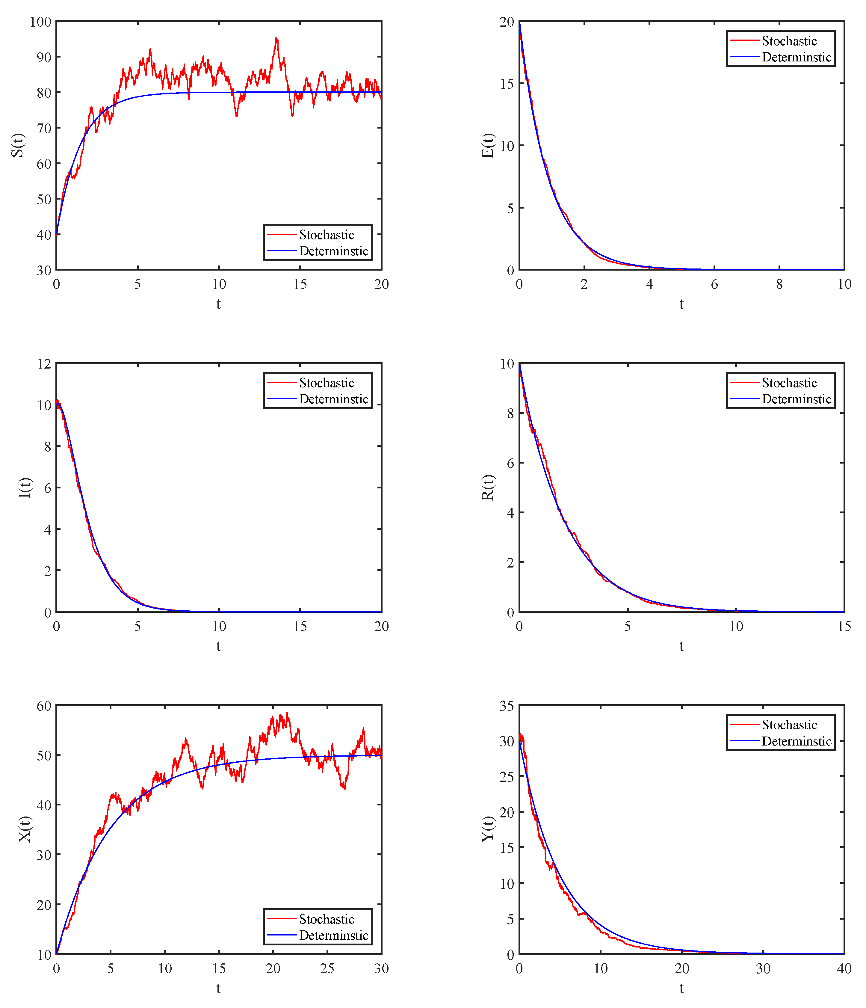
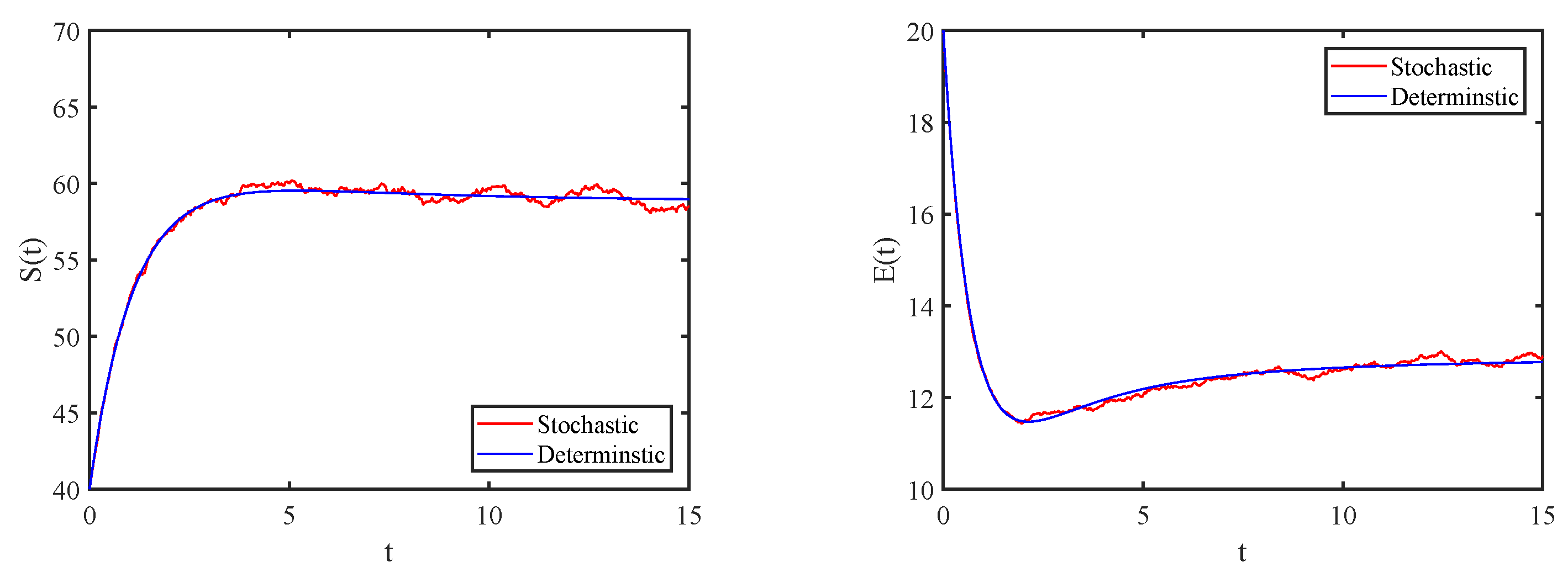
4. Numerical Simulations

In this section, we perform some numerical simulations to support the analytic results.

Taking $K=80$, $\Lambda =10$, ${\beta }_{hv}=2\times {10}^{-6}$, ${\beta }_{vh}=1\times {10}^{-6}$, ${\beta }_{hh}=5\times {10}^{-6}$, ${\alpha }_{vh}=0.02$, ${\alpha }_{hv}=0.02$, ${\alpha }_{hh}=0.02$, $c=0.1$, $d=0.1$, $\mu =0.6$, $ϵ=0.5$, $m=0.2$, $b=0.1$, $\gamma =0.1$, ${\sigma }_1=0.08$, ${\sigma }_2=0.1$, ${\sigma }_3=0.1$, ${\sigma }_4=0.08$, ${\sigma }_5=0.08$, ${\sigma }_6=0.1$, and initial condition $\left(S\right(0)=40,E(0)=20,I(0)=10,R(0)=10,X(0)=10,Y(0)=30$, we obtain ${\mathcal{R}}_0^s=0.9026<1$, and find that the Theorem 1 holds. The disease is extinct, as shown in Figure 1. The result shows that as long as the threshold ${\mathcal{R}}_0^s$ is less than 1 and the natural mortality rate of the host is greater than the critical value given in Theorem 1, the disease will eventually become extinct, which indicates that appropriate random perturbations can suppress the spread of the disease.

Similar as above, if we take $K=80$, $\Lambda =10$, ${\beta }_{hv}=0.02$, ${\beta }_{vh}=0.01$, ${\beta }_{hh}=0.005$, ${\alpha }_{vh}=0.02$, ${\alpha }_{hv}=0.02$, ${\alpha }_{hh}=0.02$, $c=0.1$, $d=0.1$, $\mu =0.6$, $ϵ=0.5$, $m=0.2$, $b=0.1$, $\gamma =0.1$, ${\sigma }_1=0.01$, ${\sigma }_2=0.01$, ${\sigma }_3=0.01$, ${\sigma }_4=0.05$, ${\sigma }_5=0.01$, ${\sigma }_6=0.01$, and initial condition $\left(S\right(0)=40,E(0)=20,I(0)=10,R(0)=10,X(0)=10,Y(0)=30$, we get ${\mathcal{R}}_0=2.037>1$, and find that Theorem 2 holds. The disease is persistent, as shown in Figure 2. The result indicates that as long as the basic reproduction number is greater than 1 and the conditions within Theorem 2 are satisfied, the disease will persist. This strongly suggests the importance of controlling the basic reproduction number in disease prevention and control.

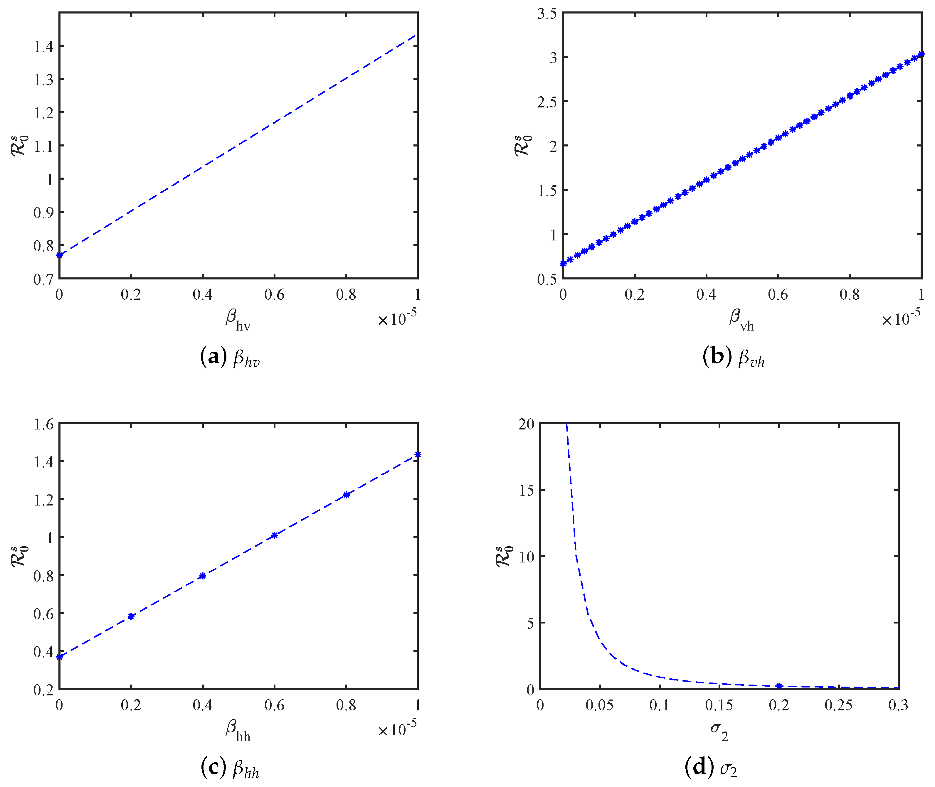
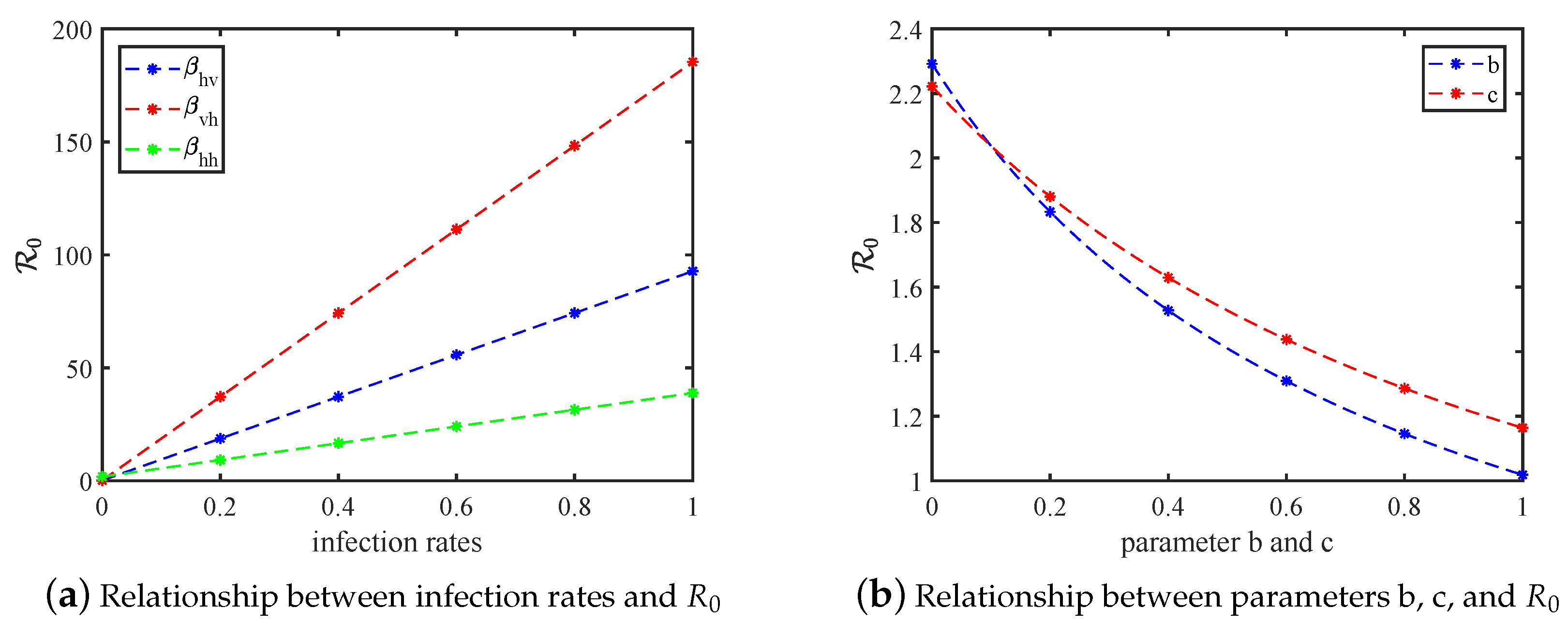
5. Sensitivity Analysis

In this section, we study the sensitivity analysis of the critical thresholds respecting the model parameters.

From the expression of (4), we can see that ${\mathcal{R}}_0^s$ is a strictly increasing function with respect to parameters ${\beta }_{hv}$, ${\beta }_{vh}$, and ${\beta }_{hh}$, and a strictly decreasing function with respect to the intensities of white noise. We provide several figures to illustrate how ${\mathcal{R}}_0^s$ varies with different contact rates. In Figure 3a–c, it is evident that as the values of ${\beta }_{hv}$, ${\beta }_{vh}$, and ${\beta }_{hh}$ increase, ${\mathcal{R}}_0^s$ quickly exceeds 1. Additionally, as shown in Figure 3d, for instance, as the value of parameter ${\sigma }_2$ decreases, ${\mathcal{R}}_0^s$ swiftly drops to 0. This indicates that the transmission of disease from vector to host or the intensities of white noise play a more significant role than the other contact rates.

From the expression of (2), we can see that $R_0$ is a function increase as parameters ${\beta }_{hv}$, ${\beta }_{vh}$, and ${\beta }_{hh}$ increase, or as parameters b and c decrease. Below, we illustrate how the basic reproduction number $R_0$ varies with different parameter values through several figures. From Figure 4a, we observe that as the values of ${\beta }_{hv}$, ${\beta }_{vh}$, and ${\beta }_{hh}$ increase, $R_0$ rapidly exceeds 1. Furthermore, the transmission from vector to host or host to vector plays a more significant role than host-to-host transmission, as illustrated in Figure 4a. Additionally, we note that as the values of b and c increase, $R_0$ decreases. However, the impact of increasing b and c is less pronounced compared to the effect of reducing contact rates (see Figure 4b). Therefore, to effectively lower $R_0$, it is advisable to both enhance plant disease resistance and reduce contact rates. For more in-depth discussions on $R_0$, refer to [1].

6. Concluding Remarks

Incorporating the concept of symmetry in a stochastic vector-borne model with nonlinear incidence can help in analyzing how robust the system’s behavior is to perturbations, whether these are stochastic fluctuations in the population sizes or changes in environmental conditions. For practical disease management, recognizing and utilizing symmetry can help in designing more effective control strategies that are robust to uncertainties in disease dynamics and environmental variations. This might include spatially or temporally targeted interventions that align with the symmetrical properties of the system.

Many plant diseases are transmitted by vectors such as insects (e.g., aphids or whiteflies). The model includes disease resistance and nonlinear incidence, allowing us to study how resistant plants impact the overall spread of a virus within a population of crops, and the way in which the rate of disease transmission changes in a nonlinear fashion with respect to the number of infected plants or vectors. The use of stochastic elements in the model (i.e., incorporating randomness) helps in reflecting the unpredictable nature of real-world disease outbreaks. Environmental factors, vector population dynamics, and random events all contribute to the spread of plant diseases. A stochastic model can better capture these complexities compared to a purely deterministic one. In this paper, we investigate a stochastic vector-borne model with plant disease resistance and nonlinear incidence (3). We give a threshold ${\mathcal{R}}_0^s$ to investigate the extinction of the disease, and use the reproduction number $R_0$ of system (1) to investigate the persistence of the disease. Our sensitivity analysis shows that random fluctuations introduced in our stochastic model can suppress disease outbreak, and the contact transmission rate strongly influences the value of ${\mathcal{R}}_0^s$. According to the sensitivity of $R_0$, we find that decreasing contact between infected individuals and susceptible individuals and increasing the resistance of plants are effective measures to control the spread of the disease.

Finally, we remark that there are quite a few aspects deserving further investigation. For example, Theorem 2 has technique conditions. And our consideration of vectors in the system is relatively simple. The system may be more realistic and complicated if we consider the vector to have six development stages as in [16], but higher dimensions cause greater difficulties in defining the threshold. Furthermore, discussing the impact of delay, seasonality, and the utilization of fractional derivatives on the deterministic system is also intriguing. However, analyzing the dynamics of the system becomes more challenging, and we plan to dedicate our future work to addressing these questions.

References

1. Fei, L.Z.; Zou, L.; Chen, X.W. Global analysis for an epidemical model of vector-borne plant viruses with disease resistance and nonlinear incidence. J. Appl. Anal. Comput. 2020, 10, 2085–2103. [Google Scholar] [CrossRef] [PubMed]
2. Jian, Y.; Gong, Y.; Fang, R. Research progress and perspective of tripartite interaction of virus-vector-plant in vector-borne viral diseases. Bull. Chin. Acad. Sci. 2017, 32, 845–855. [Google Scholar]
3. Akoth, O.P.; Pascal, M.D.; Hans-Michael, P.; Pappu, H.R. Predictive models for tomato spotted wilt virus spread dynamics, considering frankliniella occidentalis specific life processes as influenced by the virus. PLoS ONE 2016, 11, e0154533. [Google Scholar]
4. Gupta, R.; Kwon, S.Y.; Kim, S.T. An insight into the tomato spotted wilt virus (TSWV), tomato and thrips interaction. Plant Biotechnol. Rep. 2018, 12, 157–163. [Google Scholar] [CrossRef]
5. Boiteux, L.S.; Giordano, L.B. Genetic basis of resistance against two tospovirus species in tomato (Lycopersicon esculentum). Euphytica 1993, 71, 151–154. [Google Scholar] [CrossRef]
6. Kuang, Y.; Ben-Arieh, D.; Zhao, S.; Wu, C.H. Using spatial games to model and simulate tomato spotted wilt virus-western flowers thrip dynamic system. Int. J. Model. Simul. 2018, 38, 243–253. [Google Scholar] [CrossRef]
7. Whitfield, A.; Ullman, D.; German, T. Tospovirus-thrips interactions. Ann. Rev. Phytopathol. 2005, 43, 459–489. [Google Scholar] [CrossRef]
8. Wu, J.; Zhao, S.N.; Kuang, Y.; Ben-Arieh, D.; Margolis, D. New mathematical models for vector-borne disease: Transmission of tomato spotted wilt virus. In Bridging Research and Good Practices towards Patients Welfare; CRC Press: Boca Raton, FL, USA, 2014. [Google Scholar]
9. Bellomo, N.; Eftimie, R.; Forni, G. What is the in-host dynamics of the SARS-CoV-2 virus? A challenge within a multiscale vision of living systems. Netw. Heterog. Media 2024, 19, 655–681. [Google Scholar] [CrossRef]
10. Cunniffe, N.J.; Gilligan, C.A. Invasion, persistence and control in epidemic models for plant pathogens: The effect of host demography. J. R. Soc. Interface 2010, 7, 439–451. [Google Scholar] [CrossRef]
11. Jeger, M.J.; Van, D.; Mcroberts, N. Modelling transmission characteristics and epidemic development of the tospovirus–thrip interaction. Arthropod-Plant Interact. 2015, 9, 107–120. [Google Scholar] [CrossRef]
12. Morsello, S.C.; Beaudoin, A.L.P.; Groves, R.L.; Nault, B.; Kennedy, G.G. The influence of temperature and precipitation on spring dispersal of Frankliniella fusca changes as the season progresses. Entomol. Exp. Appl. 2010, 134, 260–271. [Google Scholar] [CrossRef]
13. Olatinwo, R.O.; Paz, J.O.; Brown, S.L.; Kemerait, R.C.; Hoogenboom, G. A predictive model for spotted wilt epidemics in peanut based on local weather conditions and the tomato spotted wilt virus risk index. Phytopathology 2008, 98, 1066–1074. [Google Scholar] [CrossRef] [PubMed]
14. Shaw, A.K.; Igoe, M.; Power, A.G.; Bosque-Pérez, N.; Peace, A. Modeling approach influences dynamics of a vector-borne pathogen system. Bull. Math. Biol. 2019, 81, 2011–2028. [Google Scholar] [CrossRef]
15. Shi, R.; Zhao, H.; Tang, S. Global dynamic analysis of a vector-borne plant disease model. Adv. Differ. Equ. 2014, 59. [Google Scholar] [CrossRef]
16. Czech, A.S.; Szklarczyk, M.; Gajewski, Z.; Zukowska, E.; Michalik, B.; Kobylko, T.; Strzalka, K. Selection of tomato plants resistant to a local Polish isolate of tomato spotted wilt virus (TSWV). J. Appl. Genet. 2003, 44, 473–480. [Google Scholar]
17. Ferrand, L.; Almeida, M.M.S.; Orilio, A.F.; Dal Bo, E.; Resende, R.O.; Garcia, M.L. Biological and molecular characterization of tomato spotted wilt virus (TSWV) resistance-breaking isolates from Argentina. Plant Pathol. 2019, 68, 1587–1601. [Google Scholar] [CrossRef]
18. Asfaw, M.; Kassa, S.; Lungu, E. Stochastic plant–herbivore interaction model with Allee effect. J. Math. Biol. 2019, 79, 2183–2209. [Google Scholar] [CrossRef]
19. Beddington, J.R.; May, R.M. Harvesting natural populations in a randomly fluctuating environment. Science 1977, 197, 463–465. [Google Scholar] [CrossRef] [PubMed]
20. Chen-Charpentier, B. Stochastic modeling of plant virus propagation with biological control. Mathematics 2021, 9, 456. [Google Scholar] [CrossRef]
21. Gard, T.C. Introduction to Stochastic Differential Equations; Marcel Dekker Inc.: New York, NY, USA, 1988; Volume 84, p. 19. [Google Scholar]
22. Ji, C.Y.; Jiang, D.Q.; Li, X.Y. Qualitative analysis of a stochastic ratio-dependent predator–prey system. J. Comput. Appl. Math. 2011, 235, 1326–1341. [Google Scholar] [CrossRef]
23. Jiang, D.; Shi, N.; Li, X. Global stability and stochastic permanence of a non-autonomous logistic equation with random perturbation. J. Math. Anal. Appl. 2008, 340, 588–597. [Google Scholar] [CrossRef]
24. Liu, Q.; Jiang, D.; Shi, N.; Hayat, T.; Alsaedi, A. Stationary distribution and extinction of a stochastic sirs epidemic model with standard incidence. Phys. A Stat. Mech. Its Appl. 2017, 469, 510–517. [Google Scholar] [CrossRef]
25. Liu, S.; Zhang, L.; Xing, Y. Dynamics of a stochastic heroin epidemic model. J. Comput. Appl. Math. 2019, 351, 260–269. [Google Scholar] [CrossRef]
26. Mao, X. Stochastic Differential Equations and Applications, 2nd ed.; Academic Press: Cambridge, MA, USA, 2006. [Google Scholar]
27. Rao, F. Dynamical analysis of a stochastic predator-prey model with an allee effect. Abstr. Appl. Anal. 2013, 340980. [Google Scholar] [CrossRef]
28. Wang, X.; Zhang, L.; Zhang, X.B. Dynamics of a stochastic sveir epidemic model with nonlinear incidence rate. Symmetry 2024, 16, 467. [Google Scholar] [CrossRef]
29. Zhang, L.; Liu, S.; Zhang, X. Asymptotic behavior of a stochastic virus dynamics model with intracellular delay and humoral immunity. J. Appl. Anal. Comput. 2019, 9, 1425–1442. [Google Scholar] [CrossRef]
30. Zhang, X.; Huo, H.; Xiang, H.; Shi, Q.; Li, D. The threshold of a stochastic siqs epidemic model. Phys. A Stat. Mech. Its Appl. 2017, 482, 362–374. [Google Scholar] [CrossRef]
31. Zhang, X.B.; Zhang, X.H. The threshold of a deterministic and a stochastic siqs epidemic model with varying total population size. Appl. Math. Model. 2021, 91, 749–767. [Google Scholar] [CrossRef] [PubMed]
32. Zhang, X.B.; Zheng, L. Complex dynamics of a stochastic SIR epidemic model with vertical transmission and varying total population size. J. Nonlinear Sci. 2023, 33, 108. [Google Scholar] [CrossRef]
33. Mao, X.; Marion, G.; Renshaw, E. Environmental brownian noise suppresses explosions in population dynamics. Stoch. Process. Their Appl. 2002, 97, 95–110. [Google Scholar] [CrossRef]
34. Khasminiskii, R.Z. Stochastic Stability of Differential Equations; Sijthoff & Noordhoff: Alphen Aan Den Rijn, The Netherland, 1980. [Google Scholar]
35. Strang, G. Linear algebra and its applications. Math. Comput. 1988, 435. [Google Scholar]
36. Zhu, C.; Yin, G. Asymptotic properties of hybrid diffusion systems. Siam J. Control Optim. 2007, 46, 1155–1179. [Google Scholar] [CrossRef]
Figure 1. The path S ( t ) , E ( t ) , I ( t ) , R ( t ) , X ( t ) , and Y ( t ) for deterministic model (1) and stochastic model (3), where the parameters are taken as above.
Symmetry 16 01122 g001
Figure 2. The path S ( t ) , E ( t ) , I ( t ) , R ( t ) , X ( t ) , and Y ( t ) for deterministic model (1) and stochastic model (3), where the parameters are taken as above.
Symmetry 16 01122 g002aSymmetry 16 01122 g002b
Figure 3. The dependence of R 0 s on infection rates.
Symmetry 16 01122 g003
Figure 4. Relationship between R 0 and related parameters.
Symmetry 16 01122 g004
Disclaimer/Publisher’s Note: The statements, opinions and data contained in all publications are solely those of the individual author(s) and contributor(s) and not of MDPI and/or the editor(s). MDPI and/or the editor(s) disclaim responsibility for any injury to people or property resulting from any ideas, methods, instructions or products referred to in the content.