
A Novel Discrete Linear-Exponential Distribution for Modeling Physical and Medical Data


Abstract
1. Introduction
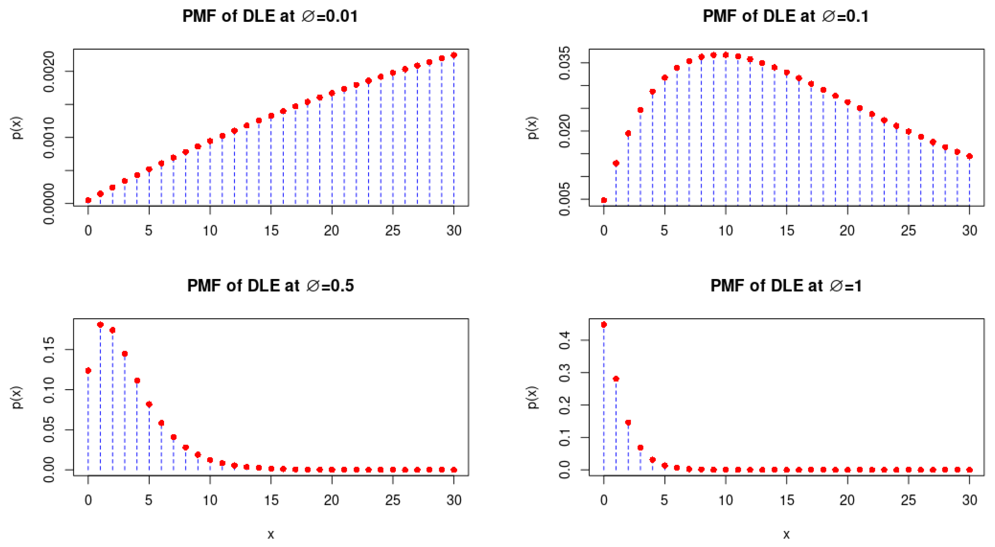
2. Some Properties of DLE Distribution
2.1. Survival and Hazard Rate Functions
2.2. Moment Generating Function (MGF)
2.3. Probability Generating Function (PGF)
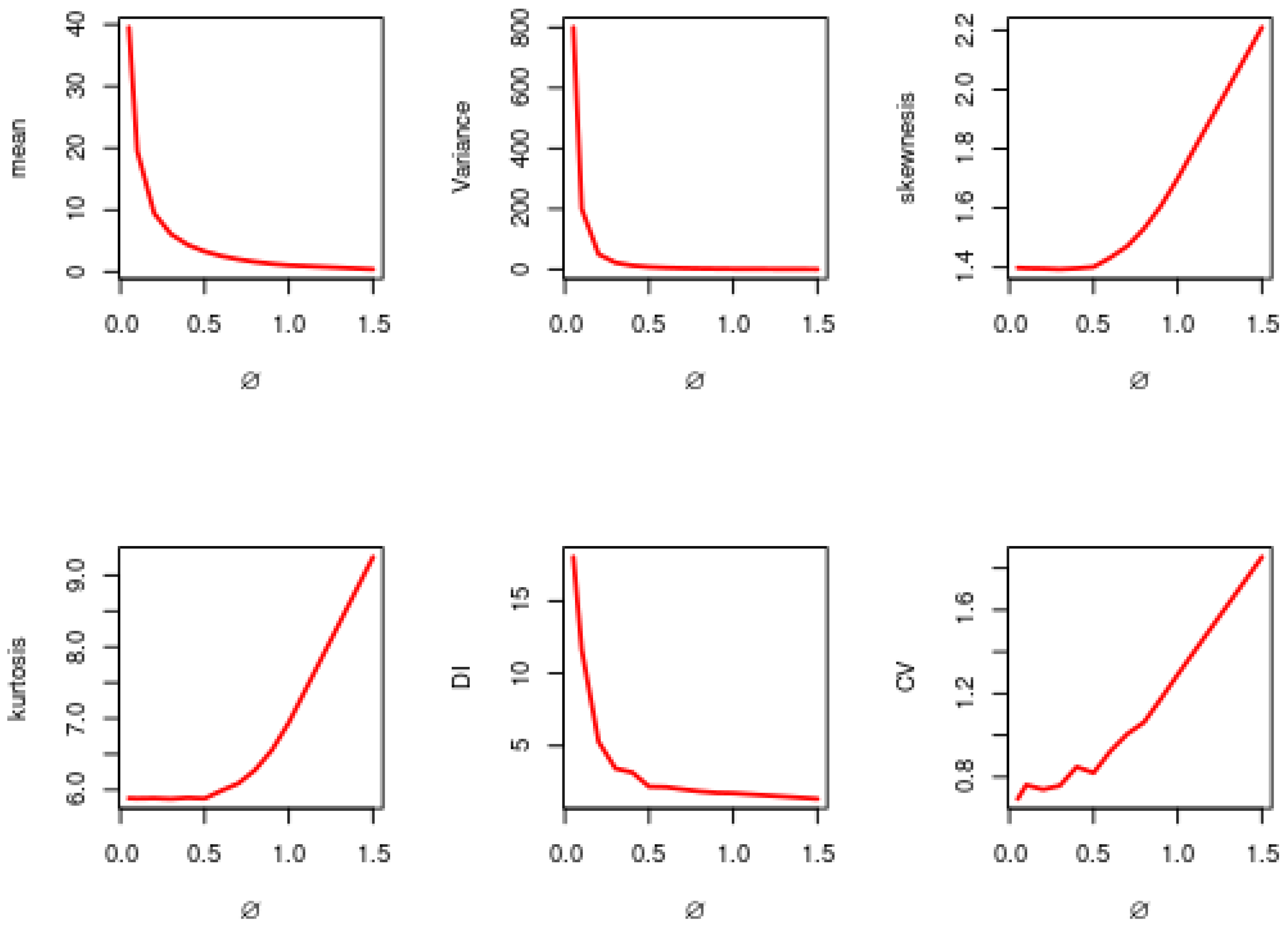
2.4. Coefficient of Variation (CV)
2.5. Dispersion Index
3. Parameter Estimation
3.1. ML Estimation
3.2. Bayesian Estimation
- Case I: Informative Prior:Assume the parameter is flowing in a gamma distribution with shape and rate parameter 1. We use the gamma prior because of its advantages of flexibility and inclusiveness of several prior beliefs used by the researcher. The hyperparameter of the gamma prior was selected in such a way that the gamma prior mean (shape/rate) was the same as the original mean (parameter value); for more details, see [15,16]. The prior density function of parameters is given by:where is positive, and then the posterior density function of given the data can be obtained as follows:
- Case II: Non-informative Prior:In this case, the unknown parameter has no or insufficient prior information. Assuming that the prior distribution of the parameter follows a uniform distribution with PDF given by:and the posterior density function of can be obtained as follows:
3.2.1. Bayesian Estimation under SELF
3.2.2. Bayesian Estimation under LINEX Loss Function
3.2.3. Bayesian Estimation under GELF
- step 1: Set the initial values
- step 2: Set i = 1.
- step 3: Generate from
- step 4: Obtain
- step 5: Generate sample U from the uniform U(0,1) distribution.
- step 6: if , then set ; otherwise
- step 7: Set i = i + 1.
- step 8: Repeat steps 2–7, M times, and obtain .
- step 9: Under SELF, obtain the Bayes estimates of as:where Q is the burn-in period.
- step 10: To obtain the credible intervals of using the algorithm proposed by [19] order as Then, the symmetric credible intervals of becomes
- step 11: Under LINEX loss function, obtain the Bayes estimates of as:
- step 12: Under GELF, obtain the Bayes estimates of as:
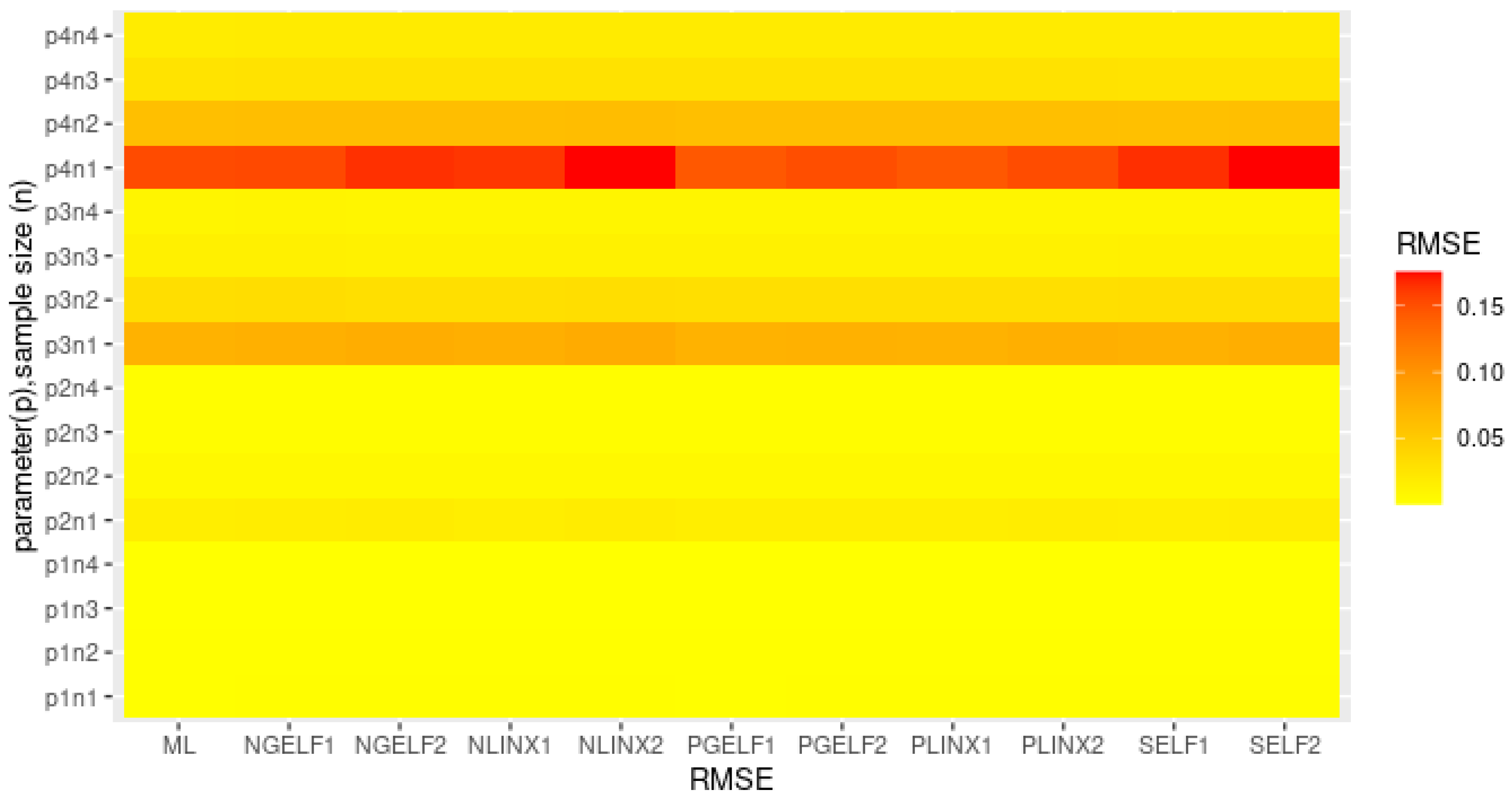
4. Simulation
- The RMSE of ML estimates and Bayes estimates for different loss function of decrease as the sample size increases.
- The estimates are asymptotically unbiased since they are more accurate as the sample size increases.
- The parameter estimates come from the best unbiased estimator when the RMSE value is near zero.
- The RMSE and length of a credible interval for the Bayesian estimates with positive weight for the asymmetric loss function are smaller than the Bayesian estimates with negative weight for the asymmetric loss function.
- A GELF with a positive weight is better than the other loss functions.
- Bayesian estimation under GELF with positive weight is better than ML estimation for all sample sizes.
5. Applications
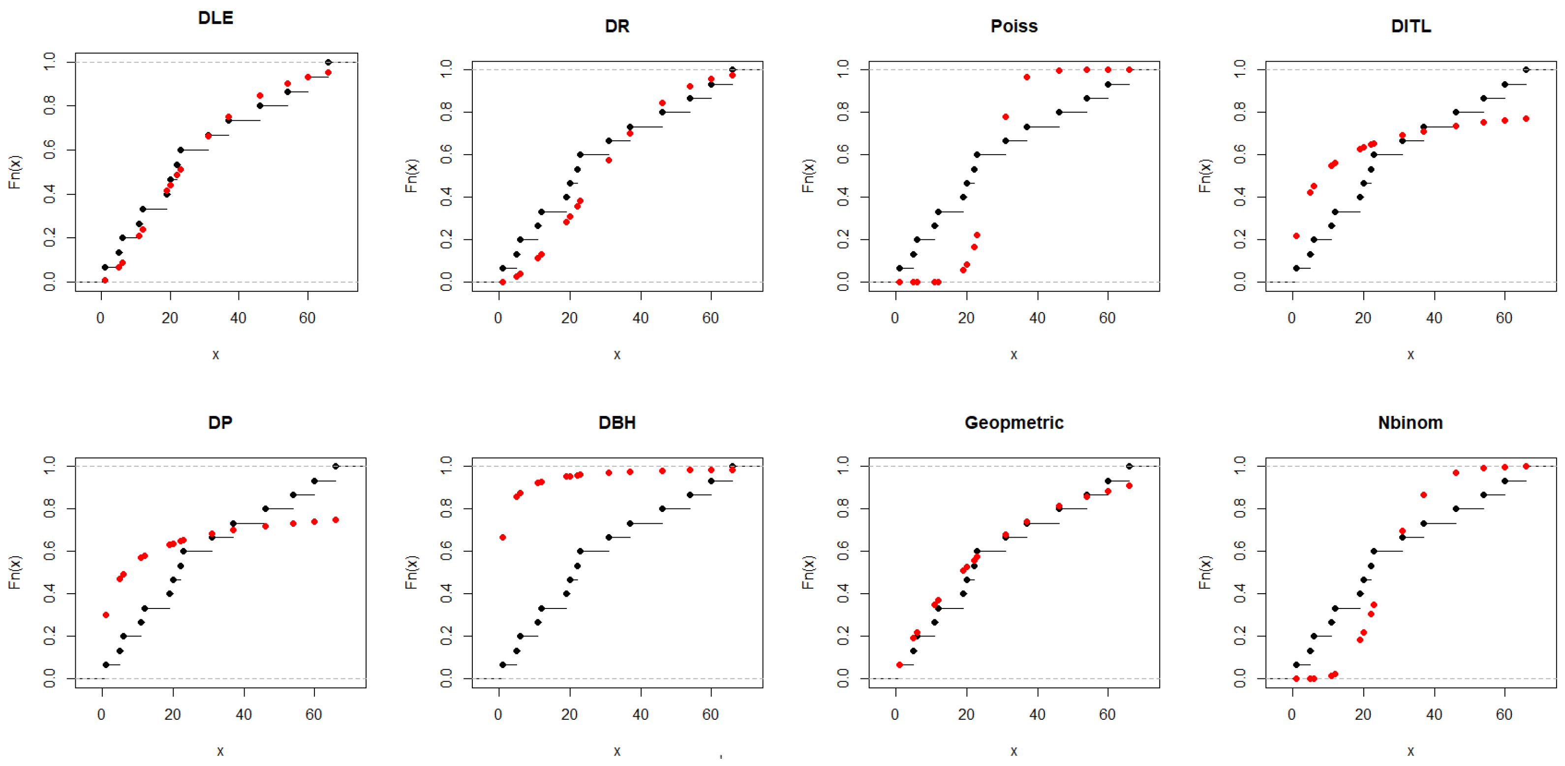
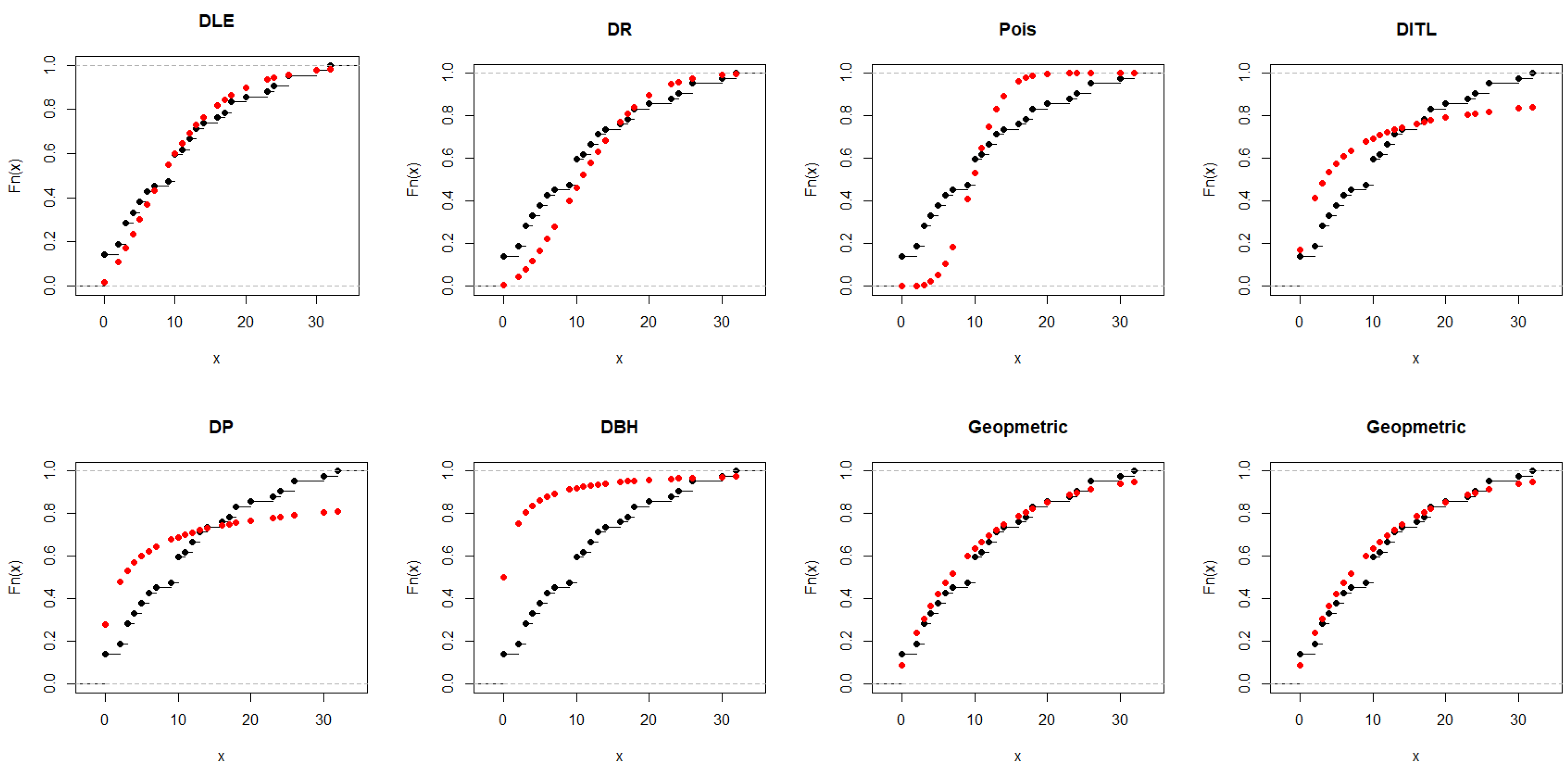
5.1. Real Data Modeling for Comparing the Competitive Discrete Models
5.1.1. Dataset I
5.1.2. Dataset II
5.1.3. Dataset III
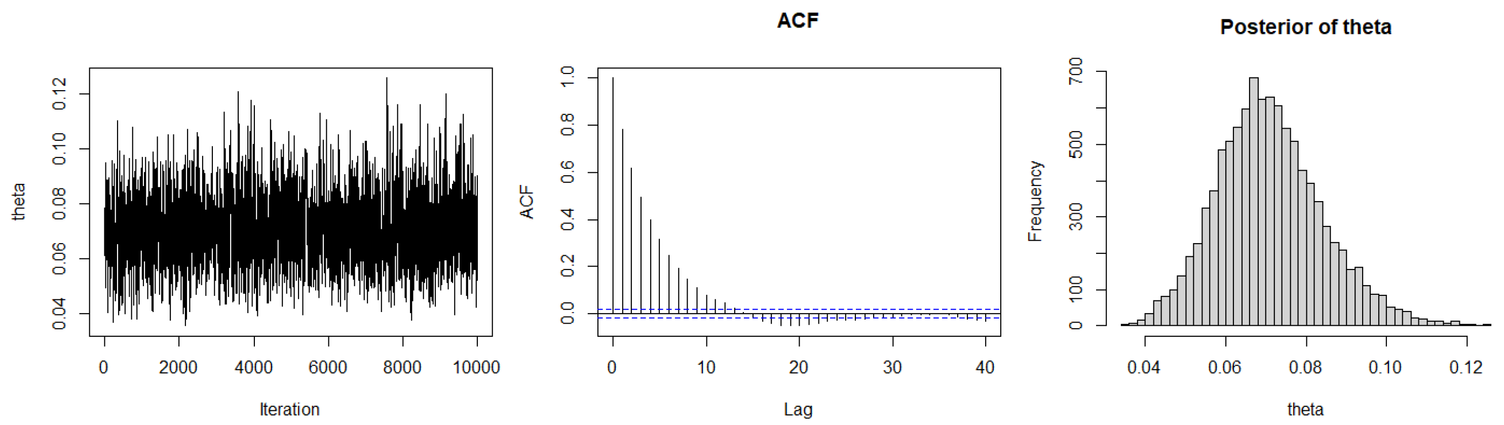
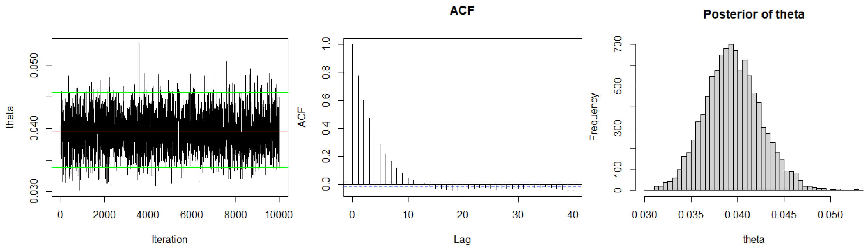
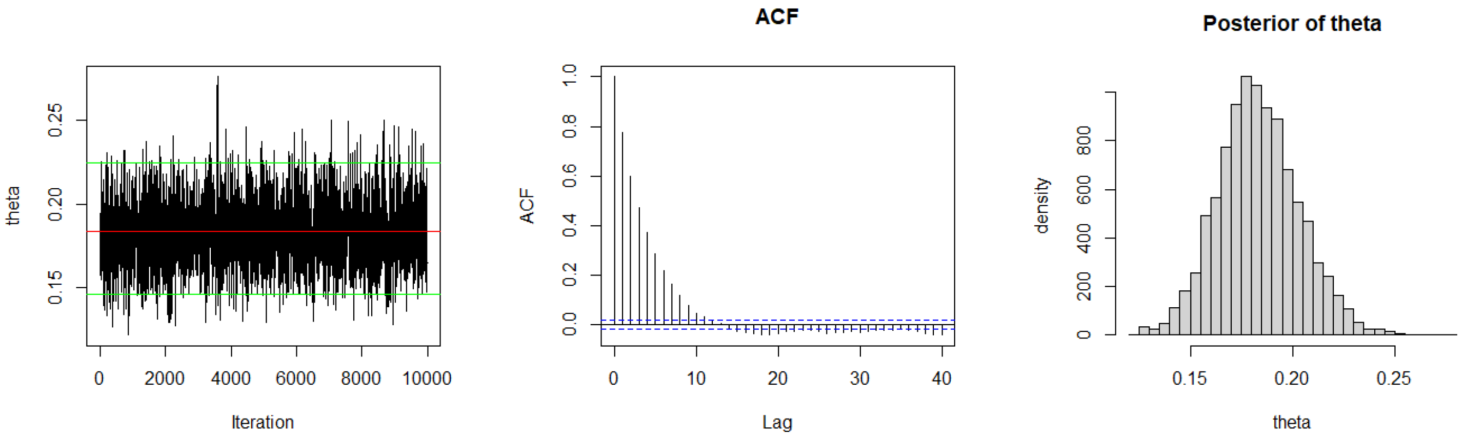
5.2. Real Data Modeling for Comparing Classical and Bayesian Estimation Methods
5.2.1. Dataset I
5.2.2. Dataset II
5.2.3. Dataset III
6. Conclusions
Author Contributions
Funding
Data Availability Statement
Acknowledgments
Conflicts of Interest
References
- Nekoukhou, V.; Alamatsaz, M.; Bidram, H. Discrete generalized exponential distribution of a second type. Statistics 2013, 47, 876–887. [Google Scholar] [CrossRef]
- El-Morshedy, M.; Eliwa, M.; Nagy, H. A new two-parameter exponentiated discrete Lindley distribution: Properties, estimation and applications. J. Appl. Stat. 2020, 47, 354–375. [Google Scholar] [CrossRef] [PubMed]
- Eliwa, M.S.; Altun, E.; El-Dawoody, M.; El-Morshedy, M. A new three-parameter discrete distribution with associated INAR (1) process and applications. IEEE Access 2020, 8, 91150–91162. [Google Scholar] [CrossRef]
- ul Haq, M.A.; Babar, A.; Hashmi, S.; Alghamdi, A.S.; Afify, A.Z. The discrete type-II half-logistic exponential distribution with applications to COVID-19 data. Pak. J. Stat. Oper. Res. 2021, 17, 921–932. [Google Scholar] [CrossRef]
- Eldeeb, A.S.; Ahsan-ul Haq, M.; Eliwa, M.S.; Cell, Q.E. A discrete Ramos-Louzada distribution for asymmetric and over-dispersed data with leptokurtic-shaped: Properties and various estimation techniques with inference. AIMS Math. 2022, 7, 1726–1741. [Google Scholar] [CrossRef]
- Alghamdi, A.S.; Ahsan-ul Haq, M.; Babar, A.; Aljohani, H.M.; Afify, A.Z.; Cell, Q.E. The discrete power-Ailamujia distribution: Properties, inference, and applications. AIMS Math. 2022, 7, 8344–8360. [Google Scholar] [CrossRef]
- Almetwally, E.M.; Abdo, D.A.; Hafez, E.; Jawa, T.M.; Sayed-Ahmed, N.; Almongy, H.M. The new discrete distribution with application to COVID-19 Data. Results Phys. 2022, 32, 104987. [Google Scholar] [CrossRef]
- El-Morshedy, M. A Discrete Linear-Exponential Model: Synthesis and Analysis with Inference to Model Extreme Count Data. Axioms 2022, 11, 531. [Google Scholar] [CrossRef]
- Alotaibi, R.; Rezk, H.; Park, C.; Elshahhat, A. The discrete exponentiated-Chen model and its applications. Symmetry 2023, 15, 1278. [Google Scholar] [CrossRef]
- Tyagi, A.; Singh, B.; Agiwal, V.; Nayal, A.S. Analysing Random Censored Data from Discrete Teissier Model. Reliab. Theory Appl. 2023, 18, 403–411. [Google Scholar]
- Alshenawy, R. A new one parameter distribution: Properties and estimation with applications to complete and type II censored data. J. Taibah Univ. Sci. 2020, 14, 11–18. [Google Scholar] [CrossRef]
- Eliwa, M.; Altun, E.; Alhussain, Z.A.; Ahmed, E.A.; Salah, M.M.; Ahmed, H.H.; El-Morshedy, M. A new one-parameter lifetime distribution and its regression model with applications. PLoS ONE 2021, 16, e0246969. [Google Scholar] [CrossRef] [PubMed]
- Chakraborty, S. Generating discrete analogues of continuous probability distributions-A survey of methods and constructions. J. Stat. Distrib. Appl. 2015, 2, 6. [Google Scholar] [CrossRef]
- Sah, B.K. One-parameter linear-exponential distribution. Int. J. Stat. Appl. Math. 2021, 6, 6–15. [Google Scholar] [CrossRef]
- Basu, S.; Singh, S.K.; Singh, U. Estimation of inverse Lindley distribution using product of spacings function for hybrid censored data. Methodol. Comput. Appl. Probab. 2019, 21, 1377–1394. [Google Scholar] [CrossRef]
- Alkhairy, I. Classical and Bayesian inference for the discrete Poisson Ramos-Louzada distribution with application to COVID-19 data. Math. Biosci. Eng. 2023, 20, 14061–14080. [Google Scholar] [CrossRef]
- Varian, H.R. A Bayesian Approach to Real Estate Assessment. In Studies in Bayesian Econometrics and Statistics in Honor of Leonard J. Savage; Elsevier (North Holland Publishing Co.): Amsterdam, The Netherlands, 1975. [Google Scholar]
- Calabria, R.; Pulcini, G. An engineering approach to Bayes estimation for the Weibull distribution. Microelectron. Reliab. 1994, 34, 789–802. [Google Scholar] [CrossRef]
- Chen, M.H.; Shao, Q.M. Monte Carlo estimation of Bayesian credible and HPD intervals. J. Comput. Graph. Stat. 1999, 8, 69–92. [Google Scholar] [CrossRef]
- Roy, D. Discrete rayleigh distribution. IEEE Trans. Reliab. 2004, 53, 255–260. [Google Scholar] [CrossRef]
- Poisson, S.D. Recherches sur la Probabilité des Jugements en Matière Criminelle et en Matière Civile: Précédées des règles Générales du Calcul des Probabilités; Bachelier: Paris, France, 1837; pp. 206–207. [Google Scholar]
- Krishna, H.; Pundir, P.S. Discrete Burr and discrete Pareto distributions. Stat. Methodol. 2009, 6, 177–188. [Google Scholar] [CrossRef]
- El-Morshedy, M.; Eliwa, M.S.; Altun, E. Discrete Burr-Hatke distribution with properties, estimation methods and regression model. IEEE Access 2020, 8, 74359–74370. [Google Scholar] [CrossRef]
- Eldeeb, A.S.; Ahsan-Ul-Haq, M.; Babar, A. A discrete analog of inverted Topp-Leone distribution: Properties, estimation and applications. Int. J. Anal. Appl. 2021, 19, 695–708. [Google Scholar]
- de Laplace, S.P. Theorie Analytique des Probabilités; par m. le Comte Laplace...; Mme ve Courcier: Paris, France, 1812. [Google Scholar]
- de Montmort, P.R.; Bernoulli, J.; Bernoulli, N. Essai d’Analyse sur les Jeux de Hazards. Seconde Édition Revue & Augmentée de Plusieurs Lettres; J. Quillau: Paris, France, 1714. [Google Scholar]
- Cui, H.; Wang, J.; Wang, C.; Liu, C.; Pi, K.; Li, X.; Xu, Y.; Tang, Z. Experimental determination of effective minority carrier lifetime in HgCdTe Photovoltaic detectors using optical and electrical methods. Adv. Condens. Matter Phys. 2015, 2015. [Google Scholar] [CrossRef]
- Lawless, J.F. Statistical Models and Methods for Lifetime Data; John Wiley & Sons: Hoboken, NJ, USA, 2011. [Google Scholar]
- Worldometers. Available online: https://www.worldometers.info/coronavirus (accessed on 1 June 2023).


| Parameter | Measures | |||||
|---|---|---|---|---|---|---|
| ϕ | Mean | Variance | Skewness | Kurtosis | DI | CV |
| 0.05 | 39.415 | 782.421 | 1.178 | 4.581 | 19.758 | 0.706 |
| 0.10 | 19.668 | 202.679 | 1.276 | 4.996 | 10.256 | 0.7199 |
| 0.20 | 9.415 | 50.197 | 1.290 | 5.165 | 5.306 | 0.748 |
| 0.30 | 6.095 | 22.251 | 1.296 | 5.125 | 3.6368 | 0.770 |
| 0.40 | 4.330 | 12.552 | 1.291 | 5.046 | 2.883 | 0.814 |
| 0.50 | 3.264 | 7.733 | 1.311 | 5.379 | 2.353 | 0.846 |
| 0.60 | 2.545 | 5.544 | 1.362 | 5.411 | 2.166 | 0.921 |
| 0.70 | 2.022 | 3.972 | 1.315 | 5.142 | 1.948 | 0.979 |
| 0.80 | 1.596 | 2.930 | 1.459 | 5.694 | 1.832 | 1.071 |
| 0.90 | 1.268 | 2.185 | 1.503 | 5.708 | 1.712 | 1.161 |
| 1.00 | 1.050 | 1.725 | 1.558 | 5.896 | 1.630 | 1.245 |
| 1.50 | 0.409 | 0.527 | 1.995 | 7.436 | 1.276 | 1.777 |
| ϕ | n | ML (Bias) (RMSE) (Length) | Bayesian Estimation | ||||
|---|---|---|---|---|---|---|---|
| SELF (Bias) (RMSE) (Length) | LINEX (Bias) (RMSE) (Length) | GELF (Bias) (RMSE) (Length) | |||||
| c = −1.5 | c = 1.5 | q = −1.5 | q = 1.5 | ||||
| 0.01 | 20 | 1.022e-2 2.189e-4 1.654e-3 5.379e-3 | 1.024e-2 2.449e-4 1.708e-3 6.578e-3 | 1.026e-2 2.637e-4 1.711e-3 6.552e-3 | 1.026e-2 2.597e-4 1.709e-3 6.547e-3 | 1.033e-2 3.255e-4 1.731e-3 6.588e-3 | 9.941e-3 −5.934e-5 1.638e-3 6.351e-3 |
| 100 | 1.009e-2 9.240e-5 7.238e-4 2.356e-3 | 1.005e-2 4.762e-5 7.297e-4 2.933e-3 | 1.001e-2 1.016e-5 7.155e-4 2.832e-3 | 1.001e-2 9.408e-6 7.154e-4 2.832e-3 | 1.002e-2 2.225e-5 7.166e-4 2.835e-3 | 9.947e-3 −5.265e-5 7.129e-4 2.816e-3 | |
| 500 | 1.000e-2 2.500e-6 3.115e-4 1.022e-3 | 1.001e-2 8.865e-6 3.131e-4 1.210e-3 | 1.002e-2 2.388e-5 3.220e-4 1.254e-3 | 1.002e-2 2.373e-5 3.220e-4 1.254e-3 | 1.003e-2 2.631e-5 3.223e-4 1.255e-3 | 1.001e-2 1.129e-5 3.209e-4 1.252e-3 | |
| 1000 | 1.001e-2 9.906e-6 2.277e-4 7.465e-4 | 1.001e-2 8.347e-6 2.326e-4 9.391e-4 | 1.000e-2 3.193e-6 2.274e-4 8.756e-4 | 1.000e-2 3.118e-6 2.274e-4 8.756e-4 | 1.000e-2 4.404e-6 2.274e-4 8.758e-4 | 9.997e-3 −3.089e-6 2.273e-4 8.748e-4 | |
| 0.1 | 20 | 1.014e-1 1.443e-3 1.684e-2 5.506e-2 | 1.020e-1 1.997e-3 1.672e-2 6.330e-2 | 1.034e-1 3.433e-3 1.710e-2 6.345e-2 | 1.030e-1 3.025e-3 1.690e-2 6.296e-2 | 1.033e-1 3.253e-3 1.731e-2 6.547e-2 | 1.000e-1 1.536e-5 1.618e-2 6.134e-2 |
| 100 | 1.002e-1 2.479e-4 6.984e-3 2.290e-2 | 1.004e-1 3.646e-4 7.272e-3 2.859e-2 | 1.007e-1 7.437e-4 7.145e-3 2.757e-2 | 1.007e-1 6.675e-4 7.127e-3 2.753e-2 | 1.002e-1 2.160e-4 7.161e-3 2.837e-2 | 1.001e-1 7.786e-5 7.057e-3 2.741e-2 | |
| 500 | 9.999e-2 −1.212e-5 3.153e-3 1.035e-2 | 1.002e-1 1.711e-4 3.103e-3 1.247e-2 | 1.000e-1 4.091e-5 3.173e-3 1.242e-2 | 1.000e-1 2.594e-5 3.172e-3 1.241e-2 | 1.003e-1 2.611e-4 3.216e-3 1.248e-2 | 9.991e-2 −9.114e-5 3.170e-3 1.239e-2 | |
| 1000 | 9.997e-2 −3.075e-5 2.253e-3 7.392e-3 | 1.000e-1 −4.288e-8 2.237e-3 8.769e-3 | 1.000e-1 2.439e-5 2.213e-3 8.683e-3 | 1.000e-1 1.691e-5 2.212e-3 8.682e-3 | 1.000e-1 4.638e-5 2.272e-3 8.747e-3 | 9.996e-2 −4.157e-5 2.211e-3 8.675e-3 | |
| 0.5 | 20 | 5.044e-1 4.449e-3 7.286e-2 2.386e-1 | 5.084e-1 8.356e-3 7.386e-2 2.966e-1 | 5.111e-1 1.107e-2 7.600e-2 2.976e-1 | 5.030e-1 3.038e-3 7.328e-2 2.894e-1 | 5.091e-1 9.129e-3 7.501e-2 2.840e-1 | 4.939e-1 −6.122e-3 7.318e-2 2.875e-1 |
| 100 | 4.993e-1 -6.802e-4 3.228e-2 1.059e-1 | 5.031e-1 3.059e-3 3.202e-2 1.239e-1 | 5.012e-1 1.186e-3 3.131e-2 1.221e-1 | 4.996e-1 −3.863e-4 3.113e-2 1.213e-1 | 4.998e-1 -1.744e-4 3.254e-2 1.255e-1 | 4.978e-1 −2.218e-3 3.118e-2 1.211e-1 | |
| 500 | 5.009e-1 8.547e-4 1.452e-2 4.757e-2 | 5.011e-1 1.075e-3 1.465e-2 5.646e-2 | 5.009e-1 8.615e-4 1.419e-2 5.472e-2 | 5.005e-1 5.468e-4 1.416e-2 5.469e-2 | 5.011e-1 1.113e-3 1.479e-2 5.767e-2 | 5.002e-1 1.804e-4 1.415e-2 5.471e-2 | |
| 1000 | 4.998e-1 −2.207e-4 1.024e-2 3.358e-2 | 5.003e-1 3.112e-4 1.010e-2 4.018e-2 | 5.002e-1 2.365e-4 1.016e-2 3.914e-2 | 5.001e-1 7.945e-5 1.015e-2 3.913e-2 | 5.001e-1 9.780e-5 1.042e-2 4.037e-2 | 4.999e-1 −1.037e-4 1.015e-2 3.914e-2 | |
| 1 | 20 | 1.033e+0 3.251e-2 1.526e-1 4.892e-1 | 1.022e+0 2.247e-2 1.656e-1 6.310e-1 | 1.042e+0 4.163e-2 1.630e-1 6.061e-1 | 1.010e+0 1.011e-2 1.451e-1 5.574e-1 | 1.029e+0 2.931e-2 1.540e-1 5.656e-1 | 1.001e+0 9.998e-4 1.453e-1 5.589e-1 |
| 100 | 1.007e+0 6.967e-3 6.140e-2 2.002e-1 | 1.005e+0 4.674e-3 6.061e-2 2.436e-1 | 1.009e+0 8.762e-3 6.223e-2 2.432e-1 | 1.003e+0 3.126e-3 6.085e-2 2.402e-1 | 1.007e+0 7.072e-3 6.218e-2 2.408e-1 | 1.001e+0 1.297e-3 6.081e-2 2.403e-1 | |
| 500 | 1.002e+0 1.674e-3 2.682e-2 8.785e-2 | 1.002e+0 2.104e-3 2.757e-2 1.071e-1 | 1.002e+0 1.542e-3 2.856e-2 1.099e-1 | 1.000e+0 4.389e-4 2.845e-2 1.096e-1 | 1.001e+0 9.337e-4 2.827e-2 1.126e-1 | 1.000e+0 7.295e-5 2.844e-2 1.096e-1 | |
| 1000 | 1.000e+0 2.484e-4 1.876e-2 6.154e-2 | 1.000e+0 3.921e-4 1.969e-2 7.778e-2 | 1.001e+0 8.097e-4 1.933e-2 7.923e-2 | 1.000e+0 2.593e-4 1.929e-2 7.908e-2 | 9.996e-1 −4.284e-4 1.929e-2 7.516e-2 | 1.000e+0 7.631e-5 1.928e-2 7.907e-2 | |
| n | ML (Bias) (RMSE) (Length) | Bayesian Estimation | |||||
|---|---|---|---|---|---|---|---|
| SELF (Bias) (RMSE) (Length) | LINEX (Bias) (RMSE) (Length) | GELF (Bias) (RMSE) (Length) | |||||
| c = −1.5 | c = 1.5 | q = −1.5 | q = 1.5 | ||||
| 0.01 | 20 | 1.022e-2 2.189e-4 1.654e-3 5.379e-3 | 1.052e-2 5.208e-4 1.809e-3 6.725e-3 | 1.052e-2 5.208e-4 1.809e-3 6.725e-3 | 1.052e-2 5.166e-4 1.806e-3 6.720e-3 | 1.058e-2 5.826e-4 1.836e-3 6.764e-3 | 1.020e-2 1.975e-4 1.690e-3 6.515e-3 |
| 100 | 1.009e-2 9.240e-5 7.238e-4 2.356e-3 | 1.006e-2 6.049e-5 7.218e-4 2.860e-3 | 1.006e-2 6.049e-5 7.218e-4 2.860e-3 | 1.006e-2 5.974e-5 7.216e-4 2.859e-3 | 1.007e-2 7.258e-5 7.237e-4 2.862e-3 | 9.998e-3 −2.285e-6 7.147e-4 2.846e-3 | |
| 500 | 1.000e-2 2.500e-6 3.115e-4 1.022e-3 | 1.003e-2 3.384e-5 3.232e-4 1.253e-3 | 1.003e-2 3.384e-5 3.232e-4 1.253e-3 | 1.003e-2 3.369e-5 3.232e-4 1.253e-3 | 1.004e-2 3.627e-5 3.236e-4 1.254e-3 | 1.002e-2 2.125e-5 3.218e-4 1.252e-3 | |
| 1000 | 1.001e-2 9.906e-6 2.277e-4 7.465e-4 | 1.001e-2 8.132e-6 2.277e-4 8.731e-4 | 1.001e-2 8.132e-6 2.277e-4 8.731e-4 | 1.001e-2 8.057e-6 2.277e-4 8.731e-4 | 1.001e-2 9.344e-6 2.277e-4 8.732e-4 | 1.000e-2 1.846e-6 2.274e-4 8.722e-4 | |
| 0.1 | 20 | 1.014e-1 1.443e-3 1.684e-2 5.506e-2 | 1.045e-1 4.538e-3 1.760e-2 6.540e-2 | 1.060e-1 6.007e-3 1.819e-2 6.480e-2 | 1.056e-1 5.588e-3 1.793e-2 6.431e-2 | 1.064e-1 6.437e-3 1.837e-2 6.490e-2 | 1.026e-1 2.579e-3 1.679e-2 6.267e-2 |
| 100 | 1.002e-1 2.479e-4 6.984e-3 2.290e-2 | 1.009e-1 8.665e-4 7.351e-3 2.888e-2 | 1.012e-1 1.243e-3 7.248e-3 2.768e-2 | 1.012e-1 1.166e-3 7.224e-3 2.764e-2 | 1.013e-1 1.330e-3 7.267e-3 2.770e-2 | 1.006e-1 5.769e-4 7.114e-3 2.750e-2 | |
| 500 | 9.999e-2 −1.212e-5 3.153e-3 1.035e-2 | 1.003e-1 2.695e-4 3.113e-3 1.248e-2 | 1.001e-1 1.405e-4 3.179e-3 1.246e-2 | 1.001e-1 1.255e-4 3.178e-3 1.246e-2 | 1.002e-1 1.579e-4 3.180e-3 1.246e-2 | 1.000e-1 8.480e-6 3.172e-3 1.244e-2 | |
| 1000 | 9.997e-2 −3.075e-5 2.253e-3 7.392e-3 | 1.001e-1 5.056e-5 2.239e-3 8.759e-3 | 1.001e-1 7.373e-5 2.215e-3 8.686e-3 | 1.001e-1 6.625e-5 2.215e-3 8.685e-3 | 1.001e-1 8.244e-5 2.216e-3 8.687e-3 | 1.000e-1 7.726e-6 2.213e-3 8.679e-3 | |
| 0.5 | 20 | 5.044e-1 4.449e-3 7.286e-2 2.386e-1 | 5.189e-1 1.887e-2 7.669e-2 2.982e-1 | 5.216e-1 2.163e-2 7.923e-2 3.040e-1 | 5.134e-1 1.340e-2 7.540e-2 2.953e-1 | 5.201e-1 2.008e-2 7.808e-2 3.007e-1 | 5.043e-1 4.292e-3 7.403e-2 2.938e-1 |
| 100 | 4.993e-1 -6.802e-4 3.228e-2 1.059e-1 | 5.052e-1 5.174e-3 3.238e-2 1.238e-1 | 5.033e-1 3.291e-3 3.154e-2 1.219e-1 | 5.017e-1 1.711e-3 3.125e-2 1.213e-1 | 5.030e-1 3.022e-3 3.145e-2 1.216e-1 | 4.999e-1 −1.200e-4 3.118e-2 1.211e-1 | |
| 500 | 5.009e-1 8.547e-4 1.452e-2 4.757e-2 | 5.015e-1 1.490e-3 1.470e-2 5.639e-2 | 5.013e-1 1.291e-3 1.423e-2 5.472e-2 | 5.010e-1 9.755e-4 1.419e-2 5.469e-2 | 5.012e-1 1.238e-3 1.422e-2 5.470e-2 | 5.006e-1 6.089e-4 1.417e-2 5.471e-2 | |
| 1000 | 4.998e-1 −2.207e-4 1.024e-2 3.358e-2 | 5.005e-1 5.209e-4 1.011e-2 4.015e-2 | 5.004e-1 4.443e-4 1.017e-2 3.920e-2 | 5.003e-1 2.872e-4 1.015e-2 3.918e-2 | 5.004e-1 4.181e-4 1.016e-2 3.919e-2 | 5.001e-1 1.041e-4 1.015e-2 3.919e-2 | |
| 1 | 20 | 1.033e+0 3.251e-2 1.526e-1 4.892e-1 | 1.043e+0 4.315e-2 1.756e-1 6.534e-1 | 1.063e+0 6.317e-2 1.755e-1 6.263e-1 | 1.030e+0 2.974e-2 1.522e-1 5.732e-1 | 1.051e+0 5.099e-2 1.653e-1 6.028e-1 | 1.021e+0 2.067e-2 1.513e-1 5.752e-1 |
| 100 | 1.007e+0 6.967e-3 6.140e-2 2.002e-1 | 1.008e+0 8.408e-3 6.131e-2 2.448e-1 | 1.013e+0 1.253e-2 6.320e-2 2.458e-1 | 1.007e+0 6.832e-3 6.148e-2 2.423e-1 | 1.011e+0 1.060e-2 6.250e-2 2.444e-1 | 1.005e+0 5.001e-3 6.132e-2 2.424e-1 | |
| 500 | 1.002e+0 1.674e-3 2.682e-2 8.785e-2 | 1.003e+0 2.831e-3 2.764e-2 1.070e-1 | 1.002e+0 2.278e-3 2.865e-2 1.101e-1 | 1.001e+0 1.173e-3 2.850e-2 1.098e-1 | 1.002e+0 1.908e-3 2.859e-2 1.100e-1 | 1.001e+0 8.077e-4 2.849e-2 1.098e-1 | |
| 1000 | 1.000e+0 2.484e-4 1.876e-2 6.154e-2 | 1.001e+0 7.598e-4 1.971e-2 7.810e-2 | 1.001e+0 1.194e-3 1.937e-2 7.903e-2 | 1.001e+0 6.434e-4 1.931e-2 7.891e-2 | 1.001e+0 1.010e-3 1.935e-2 7.898e-2 | 1.000e+0 4.606e-4 1.931e-2 7.890e-2 | |
| Models | Abbreviation | Author(s) |
|---|---|---|
| Discrete Raleigh | DR | [20] |
| Poisson | Pois | [21] |
| Discrete Pareto | DP | [22] |
| Discrete Burr-Hatke | DBH | [23] |
| Discrete Inverted Topp-Leone | DITL | [24] |
| Geometric | GEOM | [25] |
| Negative Binomial | Nbinom | [26] |
| Models | ML (S.E.) | -LL | AIC | BIC | K-S | p-Value |
|---|---|---|---|---|---|---|
| DLE | 0.071 (0.013) | 64.787 | 131.575 | 132.283 | 0.114 | 0.976 |
| DR | 24.382 (3.148) | 66.394 | 134.79 | 135.50 | 0.2160 | 0.430 |
| Pois | 27.533 (1.355) | 151.21 | 304.41 | 305.12 | 0.3810 | 0.018 |
| DITL | 0.4178 (0.107) | 74.491 | 150.98 | 151.69 | 0.3590 | 0.031 |
| DP | 0.3284 (0.084) | 77.402 | 156.80 | 157.51 | 0.4060 | 0.009 |
| DBH | 0.9992 (0.008) | 91.368 | 184.74 | 185.44 | 0.7910 | 0.000 |
| Geom | 0.035 (0.009) | 65.00 | 132.00 | 132.71 | 0.1768 | 0.673 |
| Nbinom | 0.3526 (0.018) | 88.557 | 179.11 | 179.82 | 0.3087 | 0.091 |
| Models | ML (S.E.) | -LL | AIC | BIC | K-S | p-Value |
|---|---|---|---|---|---|---|
| DLE | 0.184 (0.02) | 147.79 | 297.59 | 299.32 | 0.127 | 0.508 |
| DR | 9.874 (0.762) | 155.81 | 313.62 | 315.36 | 0.213 | 0.04 |
| Pois | 10.405 (0.498) | 240.13 | 482.26 | 483.99 | 0.328 | 0.000 |
| DITL | 0.647 (0.099) | 157.03 | 316.06 | 317.80 | 0.293 | 0.001 |
| DP | 0.472 (0.073) | 162.72 | 327.44 | 329.18 | 0.342 | 0.000 |
| DBH | 0.995 (0.000) | 177.99 | 357.97 | 359.71 | 0.614 | 0.000 |
| GEOM | 0.088 (0.013) | 142.33 | 286.66 | 288.40 | 0.159 | 0.236 |
| Nbinom | 0.801 (0.009) | 214.967 | 431.93 | 433.67 | 0.307 | 0.0007 |
| Models | ML (S.E.) | -LL | AIC | BIC | K-S | p-Value |
|---|---|---|---|---|---|---|
| DLE | 0.039 (0.003) | 330.51 | 663.027 | 665.217 | 0.172 | 0.04 |
| DR | 47.010 (2.893) | 347.23 | 696.455 | 698.644 | 0.293 | 0.000 |
| Pois | 49.742 (0.868) | 1409.8 | 2821.565 | 2823.754 | 0.497 | 0.000 |
| DITL | 0.354 (0.044) | 366.907 | 735.815 | 738.004 | 0.329 | 0.000 |
| DP | 0.286 (0.035) | 379.070 | 760.14 | 762.33 | 0.382 | 0.000 |
| DBH | 0.999 (0.002) | 461.02 | 924.04 | 926.23 | 0.812 | 0.000 |
| GEOM | 0.019 (0.002) | 324.51 | 651.02 | 653.21 | 0.085 | 0.726 |
| Nbinom | 0.570 (0.006) | 918.41 | 1838.81 | 1841.00 | 0.483 | 0.000 |
| Method | AIC | BIC | K-S | p-Value | ||
|---|---|---|---|---|---|---|
| ML | 0.071 | 131.5754 | 132.2834 | 0.11441 | 0.9766 | |
| Case I | SELF | 0.0709 | 131.5765 | 132.2846 | 0.112 | 0.981 |
| P-LINEX | 0.0708 | 131.5773 | 132.2854 | 0.111 | 0.982 | |
| N-LINEX | 0.0710 | 131.5759 | 132.284 | 0.1126 | 0.9798 | |
| P-GELF | 0.0678 | 131.6501 | 132.3582 | 0.1172 | 0.9707 | |
| N-GELF | 0.0714 | 131.5755 | 132.2836 | 0.1152 | 0.9749 | |
| Case II | SELF | 0.0735 | 131.6036 | 132.3116 | 0.12616 | 0.9464 |
| P-LINEX | 0.0734 | 131.6003 | 132.3084 | 0.1255 | 0.9485 | |
| N-LINEX | 0.0737 | 131.607 | 132.3151 | 0.1268 | 0.9441 | |
| P-GELF | 0.076 | 131.5788 | 132.2869 | 0.1115 | 0.9817 | |
| N-GELF | 0.0741 | 131.6206 | 132.3287 | 0.1292 | 0.9361 |
| Method | AIC | BIC | K-S | p-Value | ||
|---|---|---|---|---|---|---|
| ML | 0.1838 | 297.5856 | 299.3233 | 0.1269 | 0.5076 | |
| Case I | SELF | 0.1834 | 297.5837 | 299.321 | 0.1270 | 0.5068 |
| P-LINEX | 0.1831 | 297.5846 | 299.3223 | 0.1271 | 0.5063 | |
| N-LINEX | 0.1837 | 297.5833 | 299.3209 | 0.1269 | 0.5074 | |
| P-GELF | 0.1807 | 297.6085 | 299.3461 | 0.1275 | 0.5021 | |
| N-GELF | 0.1839 | 297.5832 | 299.3209 | 0.1269 | 0.5078 | |
| Case II | SELF | 0.1854 | 297.5891 | 299.3268 | 0.1299 | 0.4772 |
| P-LINEX | 0.1851 | 297.5871 | 299.3247 | 0.1291 | 0.4861 | |
| N-LINEX | 0.1857 | 297.5917 | 299.3294 | 0.1308 | 0.4684 | |
| P-GELF | 0.1827 | 297.5866 | 299.3243 | 0.1272 | 0.5056 | |
| N-GELF | 0.1859 | 297.594 | 299.3317 | 0.1315 | 0.4616 |
| Method | AIC | BIC | K-S | p-Value | ||
|---|---|---|---|---|---|---|
| ML | 0.0398 | 663.027 | 665.2167 | 0.1718 | 0.0407 | |
| Case I | SELF | 0.0397 | 663.0275 | 665.2172 | 0.1723 | 0.0398 |
| P-LINEX | 0.0397 | 663.0277 | 665.2173 | 0.1723 | 0.0397 | |
| N-LINEX | 0.0397 | 663.0274 | 665.2171 | 0.1722 | 0.0399 | |
| P-GELF | 0.0393 | 663.0447 | 665.2344 | 0.1746 | 0.0357 | |
| N-GELF | 0.0398 | 663.027 | 665.2167 | 0.1718 | 0.0407 | |
| Case II | SELF | 0.0401 | 663.0325 | 665.2221 | 0.1701 | 0.0438 |
| P-LINEX | 0.0400 | 663.0321 | 665.2217 | 0.1701 | 0.0437 | |
| N-LINEX | 0.0401 | 663.0329 | 665.2225 | 0.1700 | 0.0439 | |
| P-GELF | 0.0397 | 663.0282 | 665.2179 | 0.1725 | 0.0394 | |
| N-GELF | 0.0401 | 663.0361 | 665.2258 | 0.1697 | 0.0448 |
Disclaimer/Publisher’s Note: The statements, opinions and data contained in all publications are solely those of the individual author(s) and contributor(s) and not of MDPI and/or the editor(s). MDPI and/or the editor(s) disclaim responsibility for any injury to people or property resulting from any ideas, methods, instructions or products referred to in the content. |
© 2024 by the authors. Licensee MDPI, Basel, Switzerland. This article is an open access article distributed under the terms and conditions of the Creative Commons Attribution (CC BY) license (https://creativecommons.org/licenses/by/4.0/).
Share and Cite
Al-Harbi, K.; Fayomi, A.; Baaqeel, H.; Alsuraihi, A. A Novel Discrete Linear-Exponential Distribution for Modeling Physical and Medical Data. Symmetry 2024, 16, 1123. https://doi.org/10.3390/sym16091123
Al-Harbi K, Fayomi A, Baaqeel H, Alsuraihi A. A Novel Discrete Linear-Exponential Distribution for Modeling Physical and Medical Data. Symmetry. 2024; 16(9):1123. https://doi.org/10.3390/sym16091123
Chicago/Turabian StyleAl-Harbi, Khlood, Aisha Fayomi, Hanan Baaqeel, and Amany Alsuraihi. 2024. "A Novel Discrete Linear-Exponential Distribution for Modeling Physical and Medical Data" Symmetry 16, no. 9: 1123. https://doi.org/10.3390/sym16091123
APA StyleAl-Harbi, K., Fayomi, A., Baaqeel, H., & Alsuraihi, A. (2024). A Novel Discrete Linear-Exponential Distribution for Modeling Physical and Medical Data. Symmetry, 16(9), 1123. https://doi.org/10.3390/sym16091123