Trajectory Planning Design for Parallel Parking of Autonomous Ground Vehicles with Improved Safe Travel Corridor

Abstract

In this paper, the concept of symmetry is utilized to design the trajectory planning for parallel parking of autonomous ground vehicles—that is, the construction and the solution of the optimization-based trajectory planning approach are symmetrical. Parking is the main factor that troubles most drivers for their daily driving travel, and it can even lead to traffic congestion in severe cases. With the rise of new intelligent and autonomous vehicles, automatic parking seems to have become a trend. Traditional geometric planning methods are less adaptable to parking scenarios, while the parking paths planned by graph search methods may only achieve local optimality. Additionally, significant computational time is often required by numerical optimization methods to find a parking path when a good initial solution is not available. This paper presents a hierarchical trajectory planning approach for high-quality parallel parking of autonomous ground vehicles. The approach begins with a graph search layer to roughly generate an initial solution, which is refined by a numerical optimization layer to produce a high-quality parallel parking trajectory. Considering the high dimensionality and difficulty of finding an optimal solution for the path planning optimization problem, this paper proposes an improved safe travel corridor (I-STC) with the construction of collision constraints isolated from surrounding environmental obstacles. By constructing collision constraints of the I-STC based on the initial solution, the proposed method avoids the complexities and non-differentiability of traditional obstacle avoidance constraints, and simplifies the problem modeling the subsequent numerical optimization process. The simulation results demonstrate that the I-STC is capable of generating parallel parking trajectories with both comfort and safety.

1. Introduction

With the gradual proliferation of new intelligent and autonomous vehicles, intelligent driving is increasingly becoming a part of daily life, and the use of automatic parking systems is particularly widespread. SLAM provides the necessary environmental information and localization capabilities required for automatic parking, making it a crucial component of autonomous parking systems [1,2]. Autonomous parking can safely park vehicles in designated spots, preventing traffic accidents caused by human error and enhancing parking efficiency. The maturity of this technology not only improves the convenience and safety of parking but also showcases the potential and prospects of autonomous driving technology in the realm of smart urban transportation [3].

The geometric planning method is a common parking method [4,5]. In [6], it divided the parking process into three stages, using a Bézier curve, circular arc, and fifth-degree polynomial curve to construct the parking trajectory. The work [7] reversed parking to exiting the parking space and eliminated curvature mutations using Bézier curves. The study [8] used a series of clothoid curves and a straight line to form a continuous parking trajectory, enabling the vehicle to complete the parking maneuver from various initial orientations. The research [9] proposed a fifth-degree polynomial curve planning method for parking trajectories, which considers collisions with surrounding vehicles and achieves parking tasks in tight spaces by controlling appropriate constraint points. However, parking trajectories planned using geometric programming methods exhibit limited adaptability to the parking space and surrounding obstacles.

The artificial potential field (APF) method was first proposed by Khatib in 1986 and has since been widely applied in the field of robotics [10]. Due to its quick response time and high real-time performance, it has gradually gained traction in the domain of autonomous driving. The study [11] introduced a method different from traditional repulsion and attraction, where the repulsive force was constructed using a repulsive function to discretize obstacles and their boundary points. The results demonstrated that this method could quickly find a trajectory that satisfies constraints and ensures convergence. The work [12] added a gradient function to the traditional artificial potential field to ensure that the vehicle does not move in the direction of high gradient forces. However, in environments with complex obstacles, the artificial potential field method is prone to becoming trapped in local minima. Ref. [13] combined the artificial potential field method with neural networks, effectively avoiding the problem of local minima, although it requires a large number of training samples to support.

The use of sampling methods in automatic parking is also very extensive, including hybrid A* and RRT (rapidly exploring random tree). The study [14] proposed a new framework, the Bidirectional Rapidly Exploring Random Trees* (Bi-RRT) method that can quickly find solutions even in narrow surrounding environments. On the basis of Bidirectional Rapidly Exploring Random Trees*, the bias sampling is added to improve the accuracy of sampling [15]. The work [16] proposed GBRRT, a new motion planning algorithm based on bidirectional single query sampling, and it used the cost to target heuristic method provided by the reverse search tree to quickly find the initial feasible solution, greatly improving the running speed. A hybrid A* algorithm in [17] was used to generate a parking algorithm and ensured curvature continuity by connecting RS curves that improved driver comfort during parking. The work [18] proposed an improved A* algorithm and integrated it with the DWA algorithm, which can adapt to complex environments.

In recent years, using numerical optimization methods to solve parking trajectory problems has been in rapid development. The basic idea of optimization methods is to formulate the problem as an optimal control problem and then solve it using numerical optimization [19]. The paper [20] presented a path planning algorithm based on Modified Particle Swarm Optimization (MPSO). Unlike the standard PSO algorithm, MPSO determined the robot’s waypoint and obtained the optimal path from the starting position to the target position, and the simulation results showed that MPSO outperforms the PSO algorithm in both overall path length and CPU time. The work [21] proposed an improved fuzzy goal programming algorithm that effectively solves the problem of difficulty in determining the expected value of each optimization objective. The study [22] integrated machine learning with numerical optimization methods, significantly improving solution speed, but it depended on the number of training samples. The research [23] proposed a two-stage optimization framework, where the second stage uses gradient-based techniques to optimize trajectories obtained from particle swarm optimization in the first stage, increasing the success rate of parking in complex environments. Comparison of advantages and disadvantages in parking techniques is shown in

Table 1. Comparison of advantages and disadvantages in parking techniques.

Technique		Advantages	Disadvantages	Implemented in
Geometric planning method	Béziers	Low computational cost. Good smoothness	The computational complexity increases with the number of control points	[4,6,7]
	Polynomials	Low computational cost. Enables curve stitching	Difficult to calculate coefficients and determine equations	[9]
	Clothoids	Smooth transition, good curvature continuity	Defining a curve through integration can lead to longer processing times	[8]
Artificial potential field method		Good adaptability and fast computation time	Easy to fall into local minima	[10,11,12,13]
Sampling method	Hybrid A*	Considers the vehicle kinematic model	Not applicable to dynamic environments	[17,18]
	RRT	Fast speed, strong search ability	Low reliability in complex environments	[14,15,16]
Numerical optimization method		Can effectively consider various constraints	Long computation time	[19,20,21,22,23]

.

This paper utilizes a hierarchical planning approach for parallel parking, combining a graph search layer with a numerical optimization layer. The initial solution provided by the graph search layer serves as a warm start for the numerical optimization layer, accelerating the solving process. The numerical optimization layer can significantly optimize the trajectory quality and obtain a reliable drivable trajectory. In constructing collision constraints, an improved safe travel corridor that enhances the success rate of the solution and the quality of the resulting trajectory is proposed, which provides more drivable space in narrow areas. Finally, simulations are conducted using MATLAB to validate the approach, and comparisons are made with various traditional planning algorithms. This confirms the feasibility and superiority of the proposed hierarchical optimization-based parallel parking planning method with the I-STC.

2. Construction of Parallel Parking Planning Problem

The optimal control problem for parallel parking planning is a continuous Bolza problem with a composite performance index. This index consists of two parts: the terminal performance index Φ and the integral performance index L [21].

$$J=\Phi \left(x\left(t_0\right),t_0,x\left(t_f\right),t_f\right)+{\int }_{t_0}^{t_f}L(x\left(t\right),u\left(t\right),t)dt$$

(1)

Herein, x(t) is the state variable of the vehicle model, u(t) is control variable, t₀ is the initial time of the vehicle’s motion, and t_f is the final time of the vehicle’s motion. Solving the optimal control problem in the form of continuous Bolza is to find the allowable control variable u(t) while determining the terminal time t_f and minimizing the performance index. Among them, the state variable x(t) will be constrained by the three factors, namely vehicle motion characteristics system equation constraints (corresponding to Equation (2)), boundary constraints for the initial and final states of vehicle motion (corresponding to Equation (3)) and path constraint (corresponding to Equation (4)).

$${\displaystyle \frac{dx\left(t\right)}{dt}}=f\left(x\left(t\right),u\left(t\right),t\right)$$

(2)

$$\psi \left(t_0,t_f,x\left(t_0\right),x\left(t_f\right),u\left(t_0\right),u\left(t_f\right)\right)=0$$

(3)

$$C\left(x\left(t\right),u\left(t\right),t\right)\le 0,y\in \left[t_0,t_f\right]$$

(4)

The path constraint applies to the entire time threshold [t₀,t_f], including two parts: state variable/control variable constraint and environmental obstacle avoidance constraint. The former indicates that the vehicle’s speed, acceleration, and other state and control variables are affected by certain boundary values. The latter indicates that the vehicle cannot collide with obstacles throughout the entire parking process.

2.1. Vehicle Kinematic Model

In this paper, the vehicle’s contour is simplified to facilitate the description of vehicle motion and constraints. The actual contour of the vehicle is composed of numerous irregular curves. Retaining too many details would significantly increase the complexity of collision constraints. Therefore, this paper simplifies the vehicle’s shape to a rectangle. The simplified vehicle model is shown in Figure 1.

Herein, (x,y) represents the coordinates of the midpoint of the vehicle’s rear axle, v denotes the speed of point (x,y), a represents the longitudinal acceleration of the vehicle, θ is the heading angle of the vehicle, Ψ indicates the steering angle of the front wheels (positive for left turns), ω denotes the angular velocity of the front wheel steering angle, L_w is the wheelbase of the vehicle, L_f and L_r represent the lengths of the front and rear overhangs, and W represents the width of the vehicle. Below is this

Table 2. Important parameters used in this article.

Description	Variable	Description	Variable
Front overhang length	Lf	Heading angle	θ
Rear overhang length	Lr	Vehicle wheelbase	Lw
Vehicle width	W	Steering angle	Ψ
Acceleration of the vehicle	a	Speed of the vehicle	v
Angular velocity of the front wheel steering angle	ω	Expansion length of I-STC	l
X-coordinate of the center of the rear wheel of the vehicle	x	Y-coordinate of the center of the rear wheel of the vehicle	y
State variable of the vehicle	x(t)	Control variable of the vehicle	u(t)
Equivalent center points x coordinate for front wheel	xf	Equivalent center points y coordinate for front wheel	yf
Equivalent center points x coordinate for rear wheel	xr	Equivalent center points y coordinate for rear wheel	yr

of parameters that will be used in this paper.

A, B, C, and D represent the four vertices of the rectangular vehicle body. OXY is the global coordinate system, with all angles measured counterclockwise as positive and clockwise as negative. Since collisions during parking typically occur first at the four vertices A, B, C, and D, the relationships between the rear axle center and these four vertices are provided here:

$$\{\begin{array}{c}{x}_A=x+(L_w+L_f)cos\mathit{\theta }-\frac{w}{2}sin\mathit{\theta }\hfill \\ y_A=y+(L_w+L_f)sin\mathit{\theta }+\frac{w}{2}cos\mathit{\theta }\hfill \\ x_B=x+(L_w+L_f)cos\mathit{\theta }+\frac{w}{2}sin\mathit{\theta }\hfill \\ y_B=y+(L_w+L_f)sin\mathit{\theta }-\frac{w}{2}cos\mathit{\theta }\hfill \\ x_C=x-L_{r}cos\mathit{\theta }+\frac{w}{2}sin\mathit{\theta }\hfill \\ y_C=y-L_{r}sin\mathit{\theta }-\frac{w}{2}cos\mathit{\theta }\hfill \\ x_D=x-L_{r}cos\mathit{\theta }-\frac{w}{2}sin\mathit{\theta }\hfill \\ y_D=y-L_{r}sin\mathit{\theta }+\frac{w}{2}cos\mathit{\theta }\hfill \end{array}$$

(5)

2.2. Vehicle Kinematic Constraints

The kinematic constraints of the vehicle determine the feasibility of the planned path, which corresponds to the differential equations in Equation (1). This paper uses the well-known bicycle model to describe the kinematic constraints.

$$\left[\begin{array}{c}\dot{x}\left(t\right)\\ \dot{y}\left(t\right)\\ \dot{\theta }\left(t\right)\\ \dot{v}\left(t\right)\\ \dot{\phi }\left(t\right)\end{array}\right]=\left[\begin{array}{c}v\left(t\right)cos\theta \left(t\right)\\ v\left(t\right)sin\theta \left(t\right)\\ v\left(t\right)tan\phi \left(t\right)/L_w\\ a\left(t\right)\\ \omega \left(t\right)\end{array}\right],t\in \left[t_0,t_f\right]$$

(6)

2.3. Initial and Terminal State Constraints

The initial state corresponds to the state of the vehicle at the starting point of the parking path, while the final state should satisfy the conditions at the end of the parking maneuver. The initial and final state conditions are expressed as follows:

$$\left[\begin{array}{c}x\left(t_0\right)\\ y\left(t_0\right)\\ \theta \left(t_0\right)\\ v\left(t_0\right)\\ \phi \left(t_0\right)\end{array}\right]=\left[\begin{array}{c}{x}_{start}\\ y_{start}\\ {\theta }_{\mathrm{start}}\\ v_{start}\\ v_{start}\end{array}\right] , \left[\begin{array}{c}x\left(t_f\right)\\ y\left(t_f\right)\\ \theta \left(t_f\right)\\ v\left(t_f\right)\\ \phi \left(t_f\right)\end{array}\right]=\left[\begin{array}{c}{x}_{\mathrm{final}}\\ y_{\mathrm{final}}\\ {\theta }_{\mathrm{final}}\\ v_{\mathrm{final}}\\ {\phi }_{\mathrm{final}}\end{array}\right]$$

(7)

2.4. Path Constraints

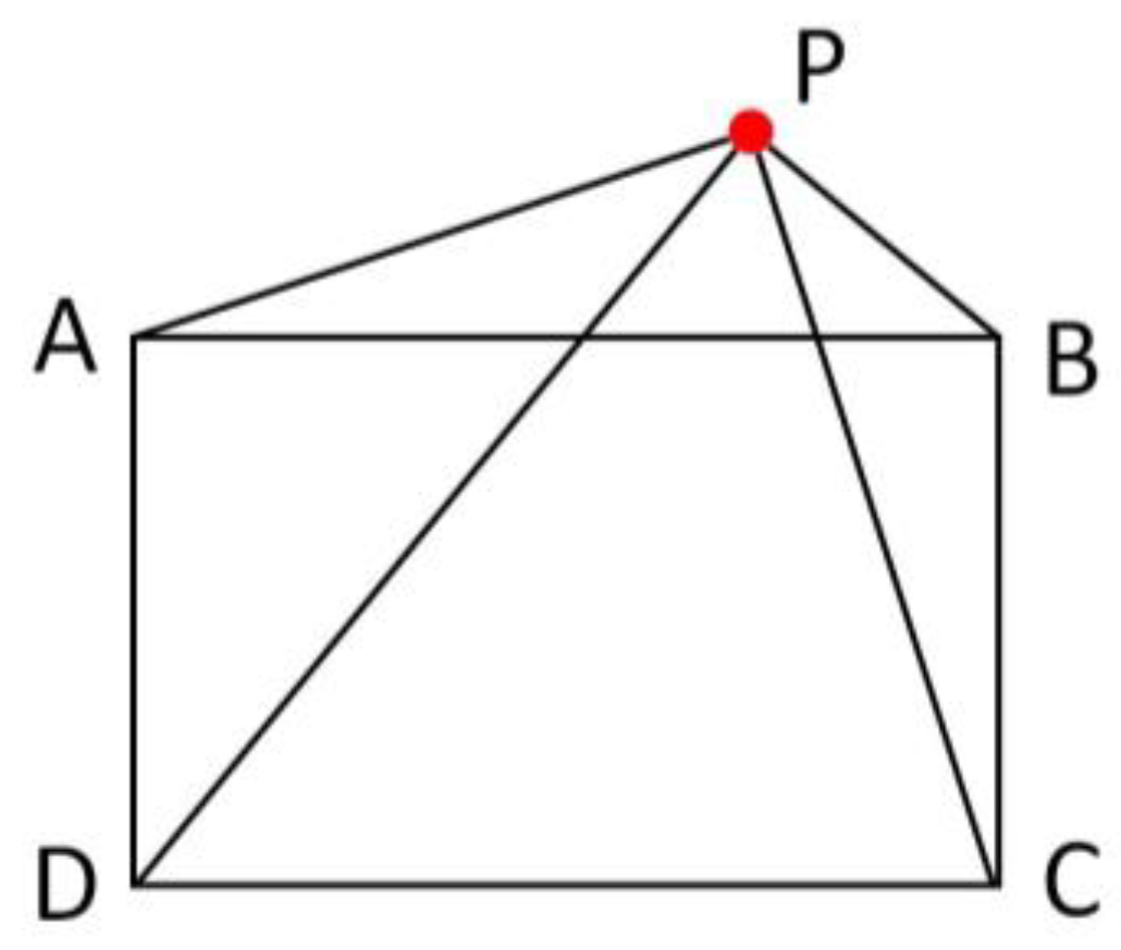
In this paper, all obstacles in the parking scenario are considered static, and the impact of dynamic obstacles is not taken into account. Collision constraints require that no point on the vehicle come into contact with any obstacle throughout the entire planning time domain. A collision between the vehicle and an obstacle is understood as an overlap between the vehicle model and the static obstacle model. A commonly used method for constructing collision constraints is the triangle area method.

The constraint expression for the triangle area method can be formulated as follows [24]:

$$S_{▱ABCD}<S_{△PAB}+S_{△PBC}+S_{△PCD}+S_{△PDA}$$

(8)

For multiple obstacles, the collision constraint shown in Figure 2 can be expressed using the triangle area method as follows:

$$S_{▱ABCD}<S_{△P_{i}AB}+S_{△P_{i}BC}+S_{△P_{i}CD}+S_{△P_{i}DA}$$

(9)

where i represents the number of obstacle vertices.

For the constraint of vehicle state tolerance values, there are limitations on each state variable and control variable:

$$\left[\begin{array}{l}-v_{\max }\\ -a_{\max }\\ -{\phi }_{\max }\\ -{\omega }_{\max }\end{array}\right]\le \left[\begin{array}{l}v(t)\\ a(t)\\ \phi (t)\\ \omega (t)\end{array}\right]\le \left[\begin{array}{l}{v}_{\max }\\ a_{\max }\\ {\phi }_{\max }\\ {\omega }_{\max }\end{array}\right],t\in [t_0,t_f]$$

(10)

2.5. Parking Cost Function

For the parking problem, the objective is typically to complete the parking maneuver in the shortest possible time. Thus, this paper adopts a time-optimal approach for the parallel parking trajectory planning optimal control problem, where t = t_f − t₀,with t_f representing the time at which parking is completed and t₀ representing the start time of parking.

minimize cost function t
s.t. kinematic constraints (6);
boundary conditions (7);
Path constraint (9) and (10).

3. Parallel Parking Trajectory Planning Based on I-STC

3.1. Initial Solution of I-STC

The A* algorithm is one of the most commonly used path planning algorithms; it is a heuristic graph search algorithm that combines the principles of Dijkstra’s algorithm with heuristic functions, enabling it to find the shortest path in directed or weighted graphs. The cost function is calculated using the following formula [25]:

$$f\left(n\right)=g\left(n\right)+h\left(n\right)$$

(11)

In this paper, f(n) represents the total cost from the starting point to the current node, g(n) denotes the actual cost from the starting point to the current node, and h(n) indicates the estimated cost from the current node to the goal point.

The initial solution used in this article is the hybrid A* algorithm. The hybrid A* path planning algorithm is based on the A* algorithm, with improvements made in various aspects such as search dimensions, cost functions, and node expansion methods [26]. These enhancements enable the generated path to better conform to the kinematic constraints of vehicle movement.

(1)

Search dimensions

The traditional A* algorithm only focuses on the horizontal and vertical coordinates of the path points, lacking navigation for the path. As a result, the generated path may involve excessive turns, which clearly cannot meet the kinematic requirements of the vehicle. The hybrid A* algorithm joins heading angle information, increasing the search dimension from two-dimensional (x, y) to three-dimensional (x, y, θ), significantly improving the quality of the generated path.

(2)

Node expansion method

The node expansion method of the hybrid A* algorithm is illustrated in Figure 3. From the position state of the parent node, expansion is carried out to six positions: front-left, front, front-right, rear-right, rear, and rear-left. This simulates the vehicle’s driving process, including straight driving, turning, and reversing maneuvers. Among these, the expansion along arcs corresponds to the motion paths at the vehicle’s maximum steering angle.

(3)

Cost function of hybrid A*

The hybrid A* algorithm introduces corresponding penalty factors to reverse and steer operations during the node expansion process in order to ensure smoother path generation.

$$f\left(n\right)=k_1\cdot P+k_2\cdot h_{schange}+k_3\cdot h_{wchange}$$

(12)

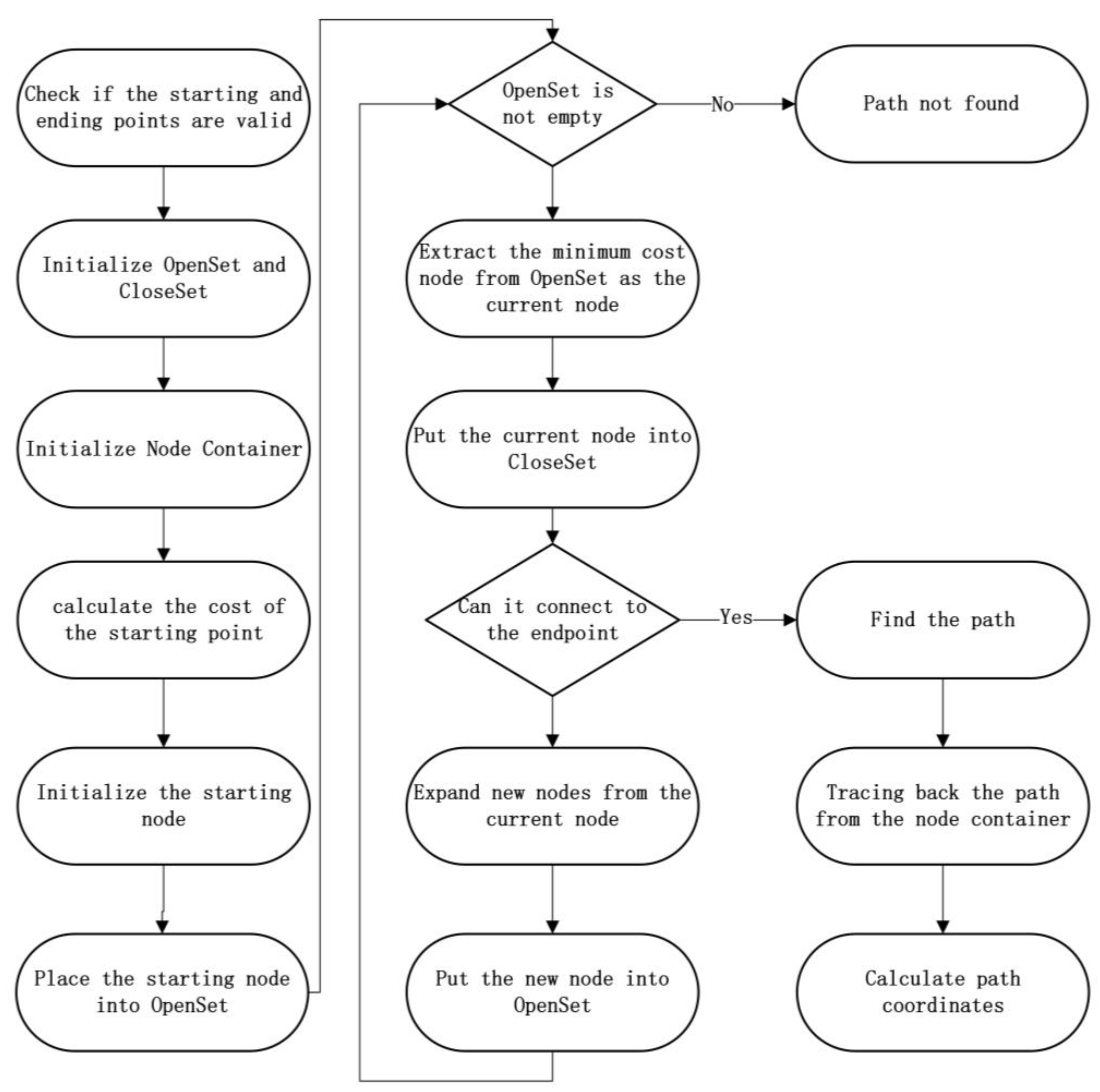
Here, P represents the path length, h_schange denotes the changes in direction during the vehicle’s movement, and h_wchange indicates the changes in the steering angle during the vehicle’s movement. k₁, k₂, k₃ are the weighted coefficients for each penalty term. When dynamic obstacles are not considered, typical parking environments are relatively simple, as parking spaces are generally defined by straightforward lines. The hybrid A* algorithm is highly effective in static environments, where its strong search capabilities allow a feasible path to be found within a short period of time. Therefore, the use of hybrid A* as the initial solution is considered an excellent choice [27,28]. The Figure 4 is the flowchart for the Hybrid A* code.

3.2. Construction of I-STC

In vehicle path planning, construction of collision constraints is the most challenging task. If the construction is improper, it will result in numerous nonlinear and non-differentiable constraints, making the optimization problem extremely difficult to solve. Therefore, constructing reasonable collision constraints is crucial in parking path planning. During parking, the driver only considers obstacles close to the vehicle and ignores those far away in the parking environment. Based on this principle, this paper introduces the concept of safe travel corridor, which originated from unmanned aerial vehicle trajectory planning and isolated unmanned aerial vehicles from surrounding environmental obstacles [29].

This paper uses the path generated by the hybrid A* algorithm as the initial solution shown in Figure 4. The generated path is a trajectory centered on the rear axle. For each path point generated, hybrid A* can create a safe travel corridor, called STC. To construct the collision constraints, we need to restrict the centers of the equivalent dual-circle model within the safety corridor area (Figure 5), to two equivalent centers, namely P_f (x_f, y_f) and P_r (x_r, y_r).

The STC is constructed through two equivalent center points, so it is necessary to separately construct STC with centers P_f and P_r. According to Equation (13), the initial solution can be transformed into trajectories of P_f and P_r. Taking the center P_f as an example, the process of generating an STC will be introduced.

$$\{\begin{array}{c}{x}_f=x+{\displaystyle \frac{1}{4}}\left(3L_W+3L_f-L_r\right)cos\theta \\ y_f=y+{\displaystyle \frac{1}{4}}\left(3L_W+3L_f-L_r\right)sin\theta \\ x_r=x+{\displaystyle \frac{1}{4}}\left(L_W+L_f-3L_r\right)cos\theta \\ y_r=y+{\displaystyle \frac{1}{4}}\left(L_W+L_f-3L_r\right)sin\theta \end{array}$$

(13)

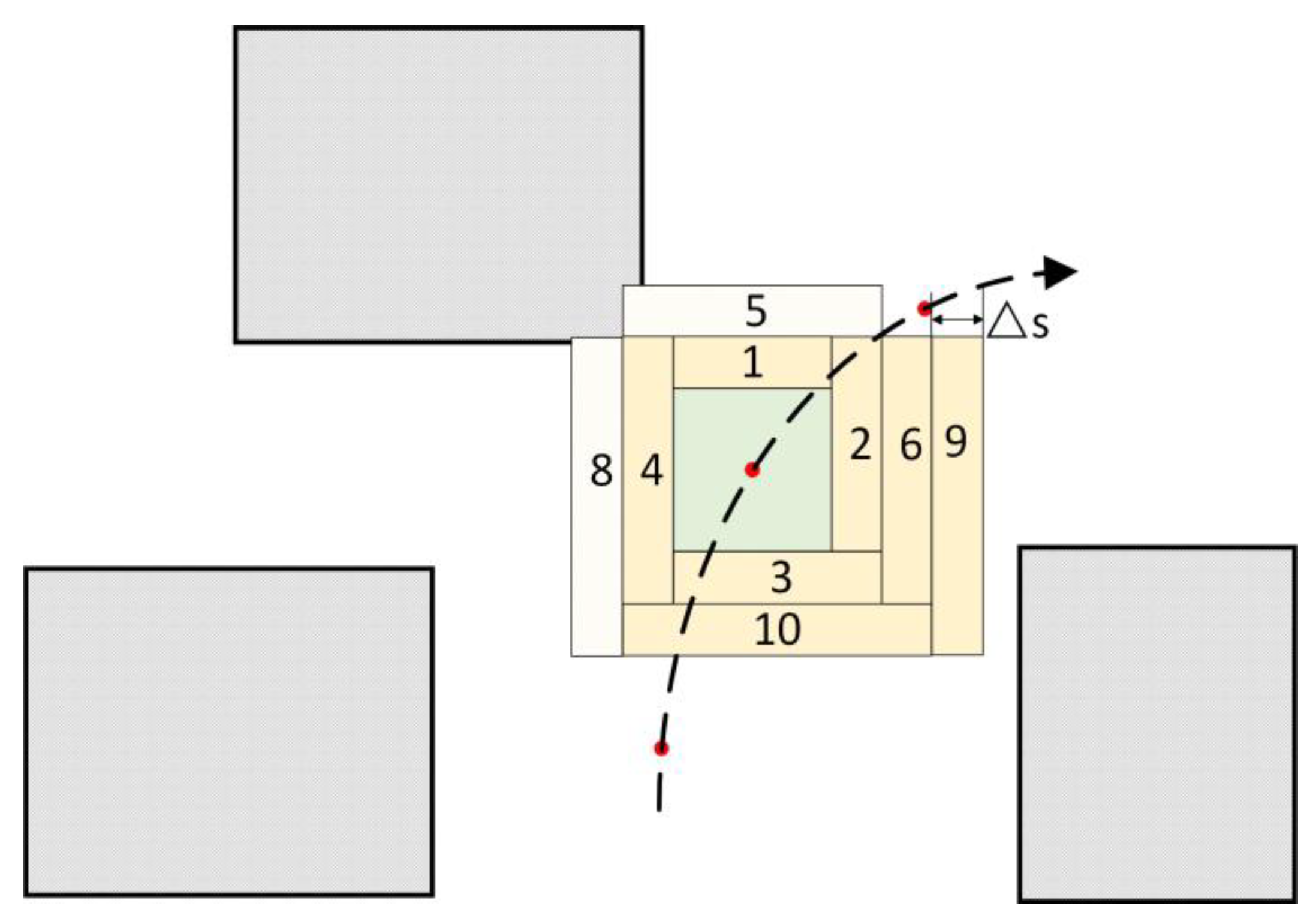
Assume there is a sampling point P_f with coordinates (x_f,y_f). Using this point as the center to generate an initial square region, then expand the area by a step size △s in the order of up, right, down, and left. Each expansion generates a rectangular area with a width of △s. The expanded area is then checked for collisions with obstacles. If no collision occurs, the newly expanded area is added to the STC. If collision occurs, the growth in that direction stops, and the STC is no longer expanded in that direction. The STC will continue to expand in directions without collisions until it reaches the preset maximum length (Figure 6). Finally, the lengths of the expansions in each direction are recorded.

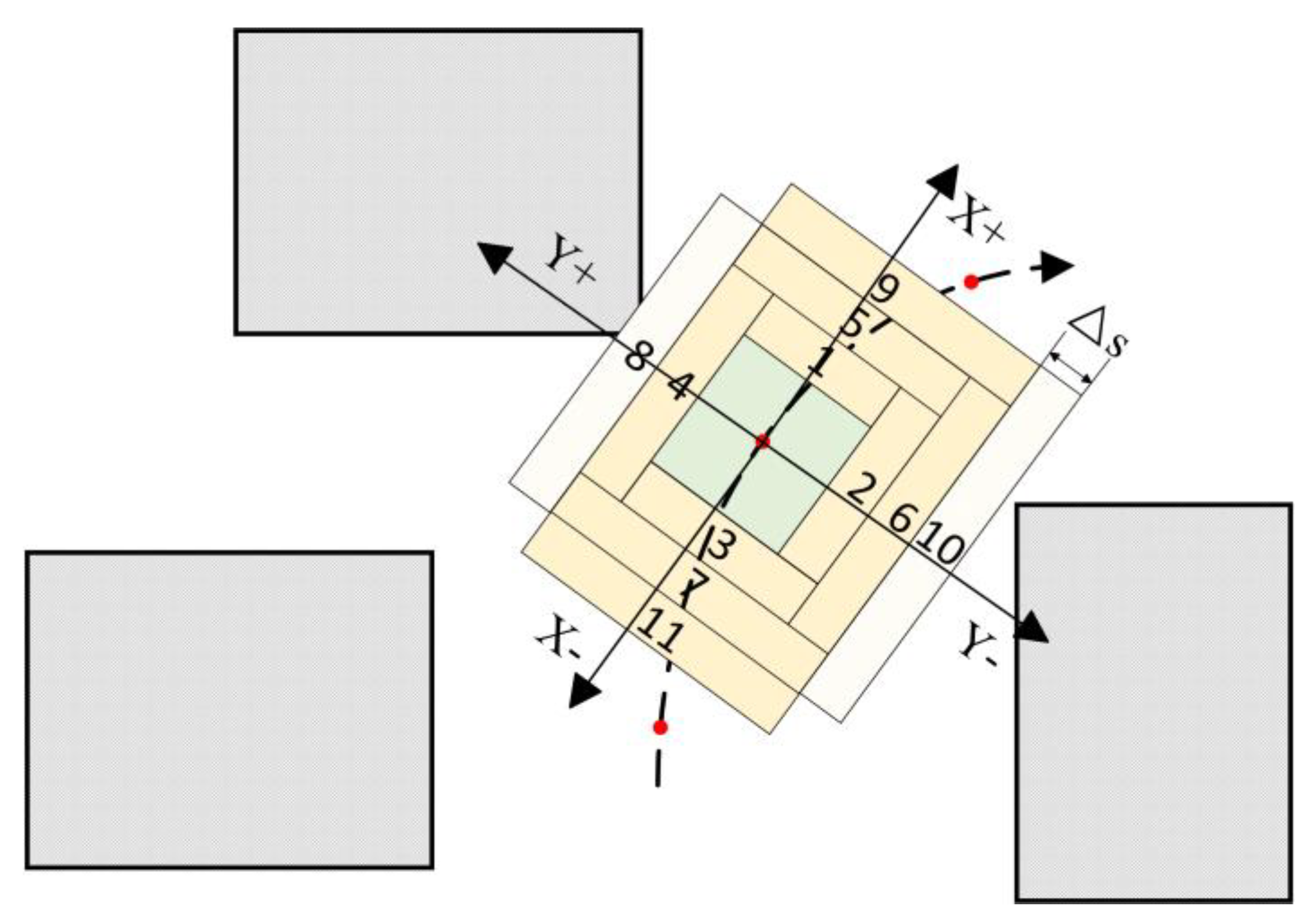
This paper proposes an improved safe travel corridor (I-STC). The I-STC extends from the original two-dimensional level to three-dimensional. I-STC is extended based on the heading angle of the vehicle. The expansion principles are similar to those for the STC. Expansion follows the direction of the vehicle’s heading angle and is divided into four directions (X+,Y−,X−,Y+) (Figure 7). Finally, the I-STC region forms a rectangular space with its axis parallel to the vehicle coordinate system.

After constructing the I-STC, at each sampling moment, the collision constraints are built by restricting the vehicle’s two equivalent centers (P_f and P_r) within their respective I-STCs. Here, the specific expression for constructing the collision constraints is provided:

$$\begin{array}{c}-l_{x^{-},f,i}\le \left(x_{f,i}-x_{sf,i}\right)cos({\theta }_{sf,i})+\left(y_{f,i}-y_{sf,i}\right)sin({\theta }_{sf,i})\le l_{x^{+},f,i}\\ -l_{y^{-},f,i}\le -\left(x_{f,i}-x_{sf,i}\right)sin({\theta }_{sf,i})+\left(y_{f,i}-y_{sf,i}\right)cos({\theta }_{sf,i})\le l_{y^{+},f,i}\\ -l_{x^{-},b,i}\le \left(x_{r,i}-x_{sr,i}\right)cos({\theta }_{sb,i})+\left(y_{r,i}-y_{sr,i}\right)sin({\theta }_{sr,i})\le l_{x^{+},r,i}\\ -l_{x^{-},b,i}\le -\left(x_{r,i}-x_{sr,i}\right)cos({\theta }_{sb,i})+\left(y_{r,i}-y_{sr,i}\right)sin({\theta }_{sr,i})\le l_{x^{+},r,i}\end{array}$$

(14)

Here, i indicates the number of sampling points; f and r represent two equivalent center points; (x, y) indicate the center coordinates of the rear axle of the vehicle; (x_s, y_s) indicate the starting point coordinates of I-STC; l_x+, l_x−, l_y+, l_y− respectively represent the lengths of expansion in the four directions of I-STC; θ_s indicates the heading angle of the I-STC.

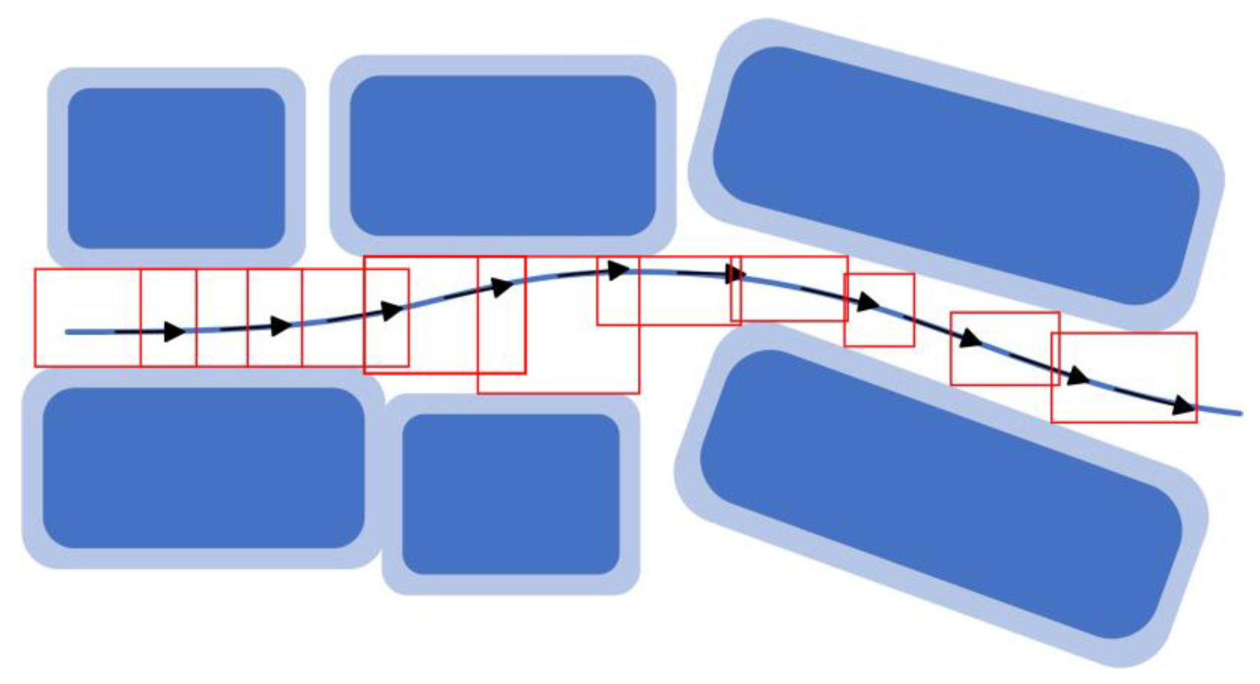
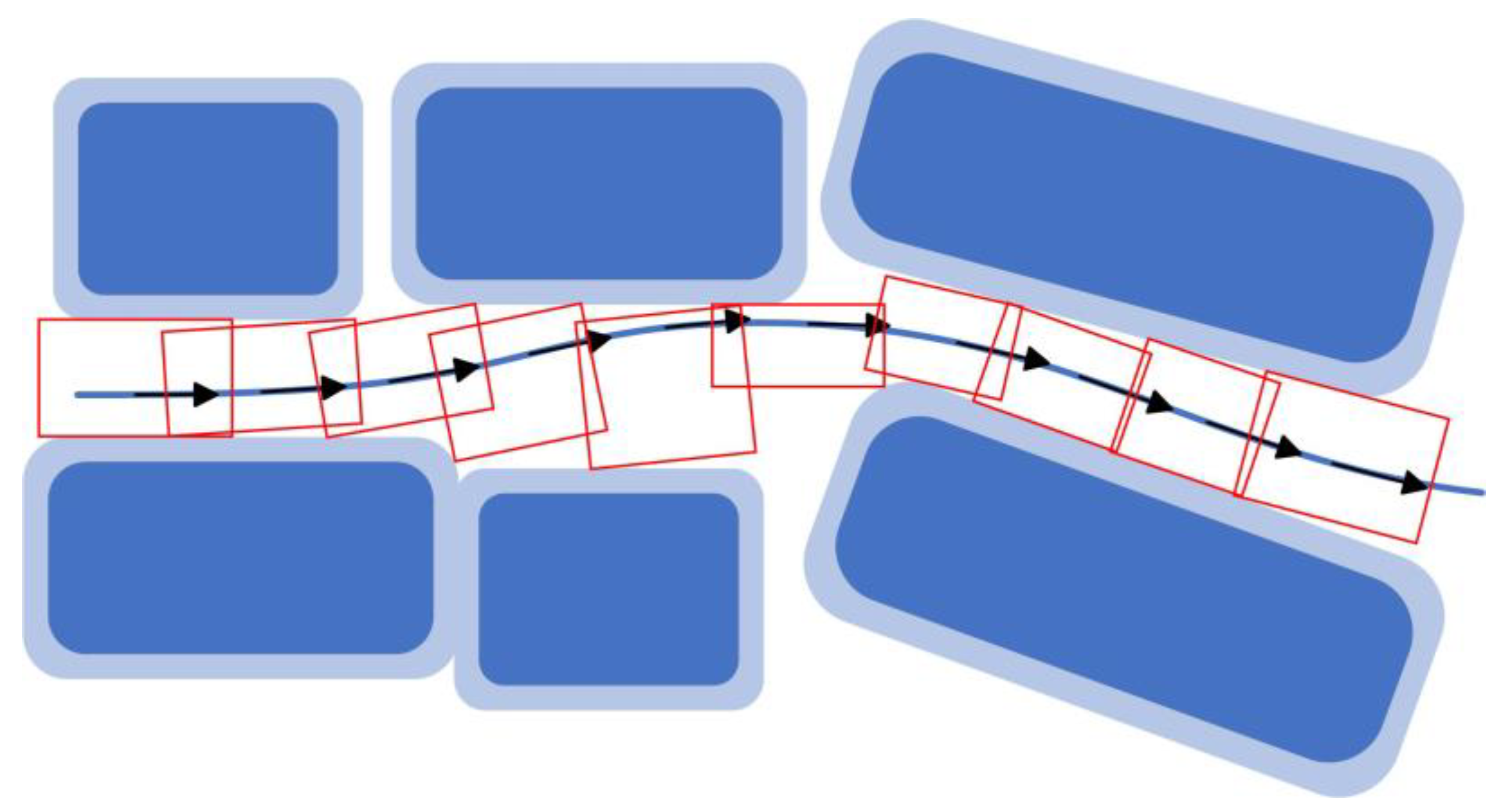
When the STC does not consider the vehicle’s heading angle, the generated safety corridor region can be quite narrow (Figure 8). This means that the drivable area of the trajectory at that moment is reduced, making it difficult to ensure that the trajectory remains within a safe region at the subsequent sampling moments. This undoubtedly increases the difficulty of solving the optimization problem. In contrast, the I-STC can generate a wider safety corridor even in narrow environments (Figure 9), facilitating the solution of the subsequent optimization problem.

Based on the collision constraint constructed by the I-STC, the entire parking problem can be expressed as follows:

minimize cost function t
s.t. kinematic constraints (6);
boundary conditions (7);
Path constraint (10) and (14).

The optimization problem can be discretized over time, dividing the complete planning problem into N segments (N depends on the path of the initial solution). The transformed optimization problem becomes a typical nonlinear programming (NLP) problem, which can be solved using some standard solvers. In this paper, the solver used is IPOPT.

4. Simulation and Results

This section presents the parallel parking simulation results based on the I-STC method. The parameters related to the vehicle and the parameters related to the parallel parking task are recorded in

Table 3. Simulation parameters.

Description	Scale	Unit
Length of parking space	7, 6.5	m
Width of parking space	2.2	m
Parking channel width	4	m
Front overhang length	0.5	m
Rear overhang length	0.5	m
Vehicle length	4	m
Vehicle width	1.8	m
Vehicle wheelbase	3	m
Bound of steering angle	0.68	rad
Bound of acceleration	1	m/s2
Bound of velocity	2	m/s
Bound of steering angular velocity	0.34	rad/s
Hybrid A* growth step size	0.3	m
Maximum length of I-STC	3	m
Expansion step size of I-STC	0.1	m

. Two parking slot lengths are constructed to verify the effectiveness of this method.

The initial position of the vehicle is set to (8, 3.6), and the parking endpoint is set to (1.5, 1.05). All of the simulation results were generated by applying MATLAB 2020a in Windows 10 with an Intel Core i7-9750H CPU.

4.1. Scenario 1

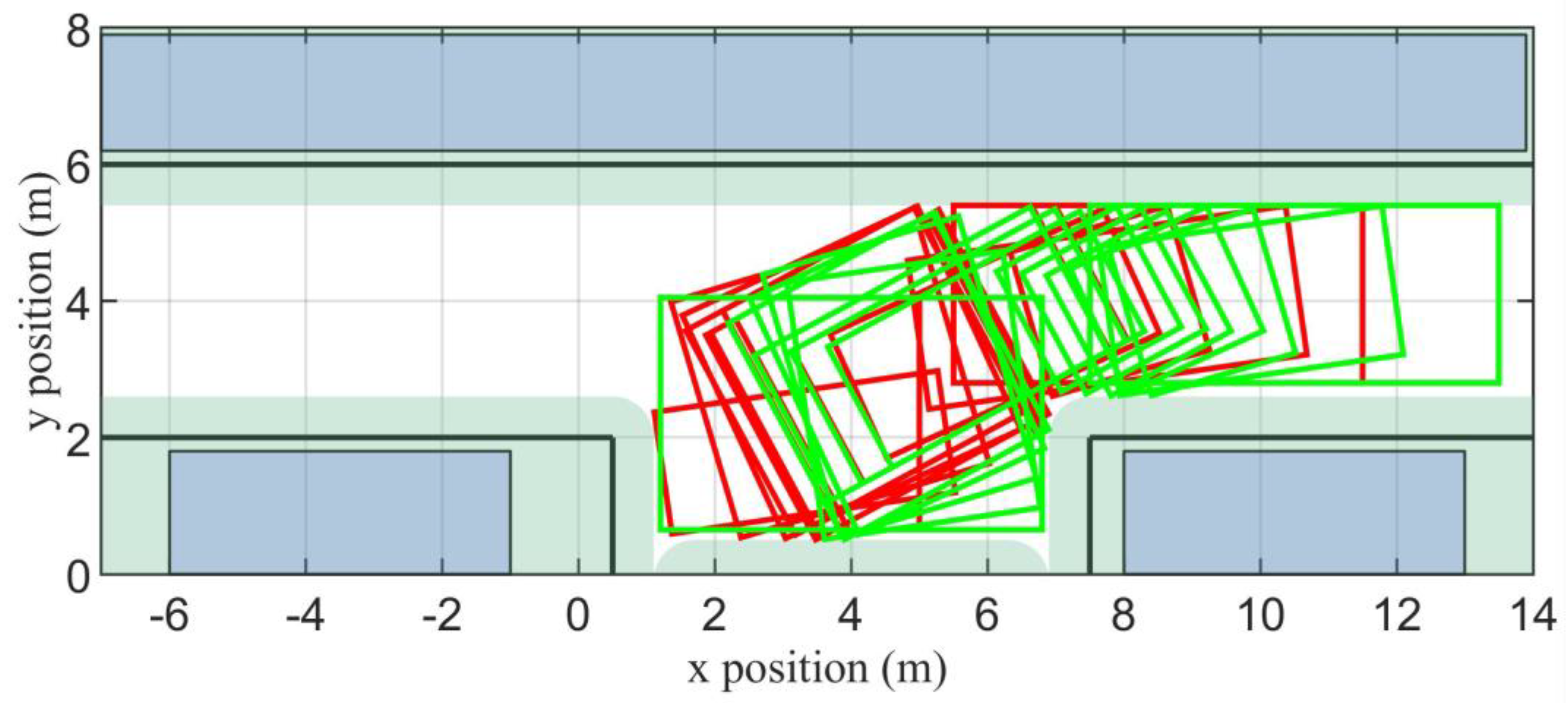
In this scenario, the defined parking slot length is 7 m, which is a standard parking slot length. The I-STC generated based on the initial solution using the hybrid A* algorithm is shown in Figure 10. The red rectangles represent the I-STC for P_r, while the green rectangles represent the I-STC for P_f.

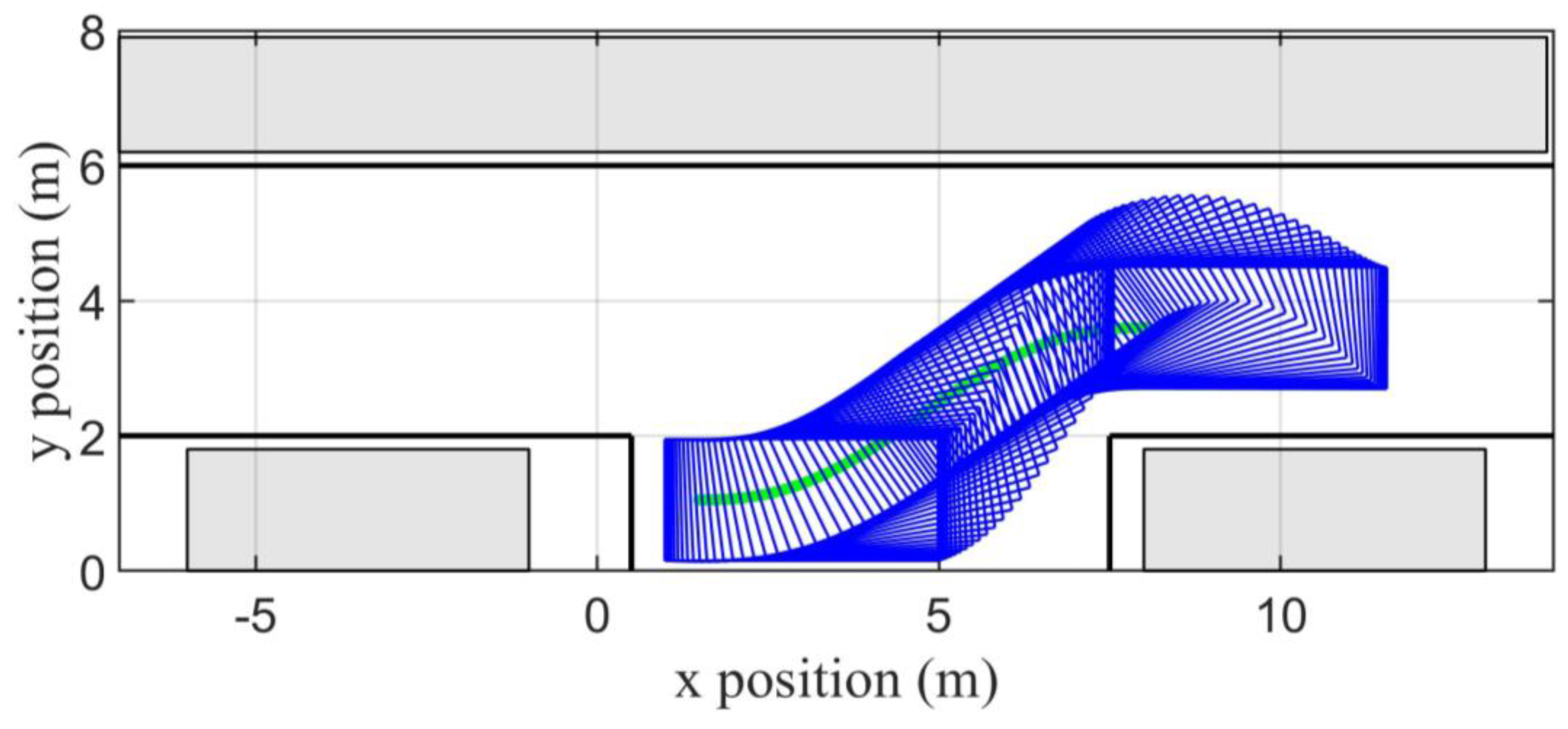
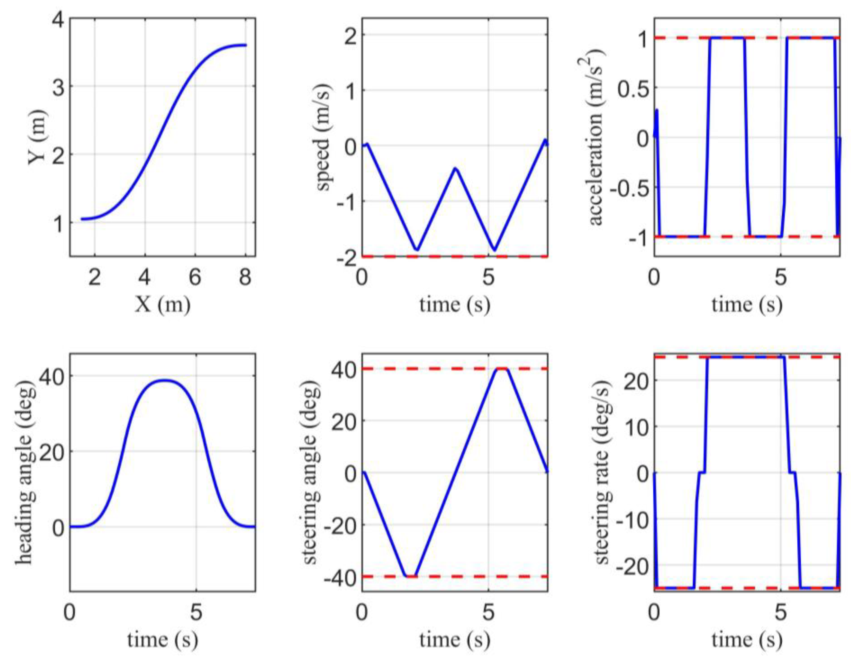
The trajectory solved using the constraints based on the I-STC is shown in Figure 11. Figure 12 illustrates the state and control input data for the parking trajectory. It can be observed that, since the starting point of the parking task is relatively close to the parking slot, the vehicle first moves forward a short distance to adjust to an appropriate state, then performs a significant reverse maneuver, and finally straightens the front of the vehicle.

4.2. Scenario 2

In this scenario, the defined parking slot length is 6.5 m, which is a relatively short parking space, and it is expected that the vehicle will need to perform multiple adjustments. The I-STC generated based on the initial solution is shown in Figure 13. Due to the reduced length of the parking slot, the quality of the initial solution from the hybrid A* algorithm is not very high. The trajectory generated by the hybrid A* algorithm involves multiple adjustments, resulting in a significantly higher number of I-STCs compared to Scenario 1.

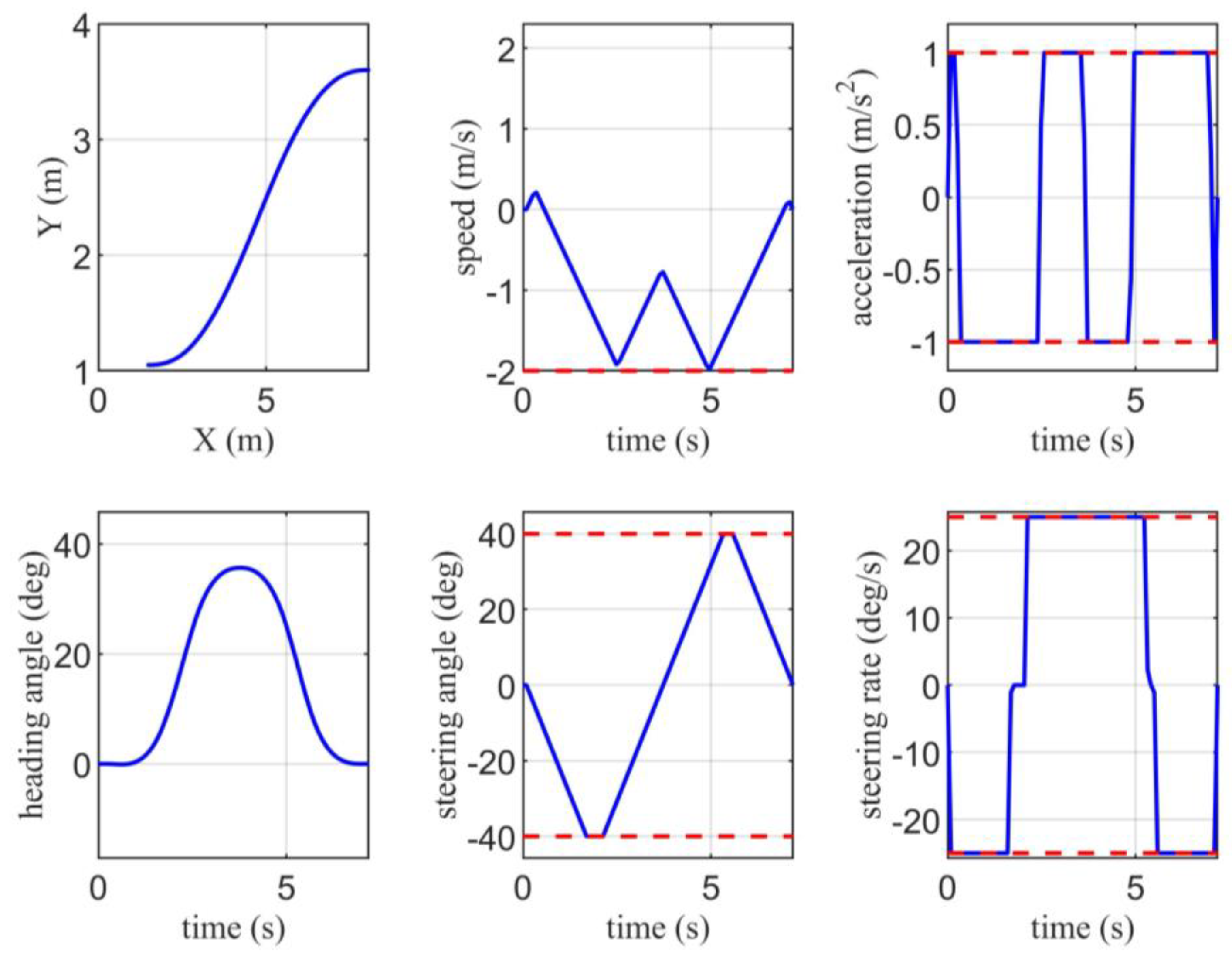
Under the constraints of this corridor, the generated trajectory is shown in Figure 14. Figure 15 displays the state and control input data for this parking trajectory. Due to the 0.5 m reduction in parking slot length, the difficulty for the vehicle to park increases. Observing the control input data, the vehicle first makes a small forward movement, with a length slightly greater than the forward movement in Scenario 1. Then, the vehicle performs a significant reverse maneuver, ultimately parking in the slot and adjusting to the set final state.

4.3. Comparison against Other Techniques

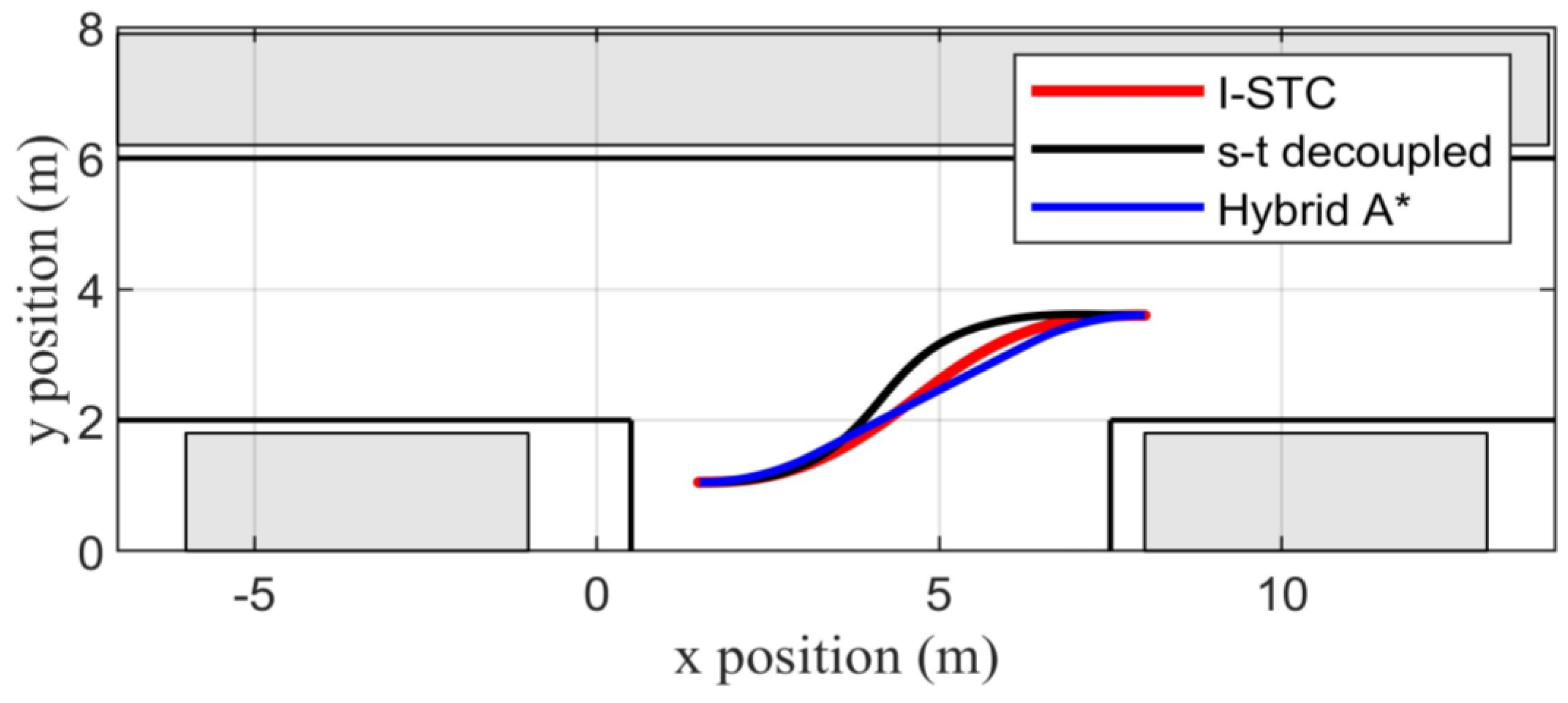
This paper compares the proposed method with the hybrid A* algorithm and the spatio-temporal decoupled numerical optimization method [24]. For a 7 m parking slot, as is shown in Figure 16 and Figure 17, there is not much difference in the quality of the three trajectories. Since the spatio-temporal decoupled method progresses from the parking target position to the parking starting position, which is a reverse process compared to parking, the vehicle’s heading angle is relatively larger, and the parking length is also longer. The blue trajectory represents the hybrid A* trajectory; the red trajectory is generated based on the I-STC method, and the black trajectory is generated based on the spatio-temporal decoupled method (abbreviated as s-t decoupled in Figure 16).

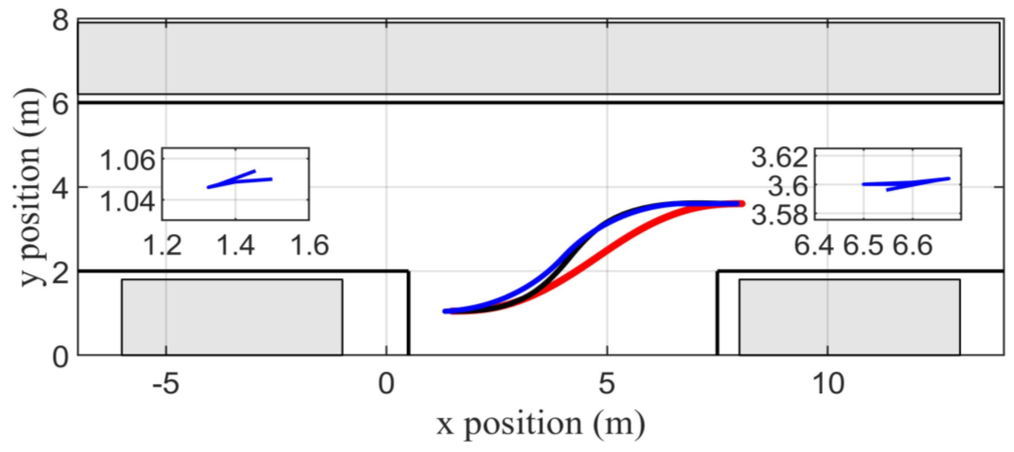
For a 6.5-m parking slot, as is shown in Figure 17, the enlarged trajectory diagram shows a significant decline in the trajectory quality of the hybrid A* algorithm, with three intermediate adjustment maneuvers. Although the trajectory generated by the spatio-temporal decoupled method is of high quality, its solving time is much longer than that of the other two methods. In contrast, the trajectory generated based on the I-STC has a relatively short solving time and also maintains high quality.

Detailed data can be found in

Table 4. Comparison of important parameters.

Description		Length of Planned Path (m)	Number of Speed Reversals	CPU Time (s)
Scenario 1	I-STC	7.1962	2	1.2384
	Spatio-temporal decoupled	7.3688	0	14.5823
	Hybrid A*	7.0708	0	0.2872
Scenario 2	I-STC	7.2681	2	2.5726
	Spatio-temporal decoupled	7.3688	0	28.3473
	Hybrid A*	7.9354	3	0.5218

. This paper selects three indicators for comparison, including length of planned path, number of speed reversals, and CPU time. It can be observed that, for a 7 m parking slot, the trajectory generated by the hybrid A* algorithm is of decent quality. Although the trajectory generated by the I-STC method involves two instances of reversing, these are small adjustments to the vehicle’s heading and do not affect actual driving. On the other hand, the spatio-temporal decoupled method takes a longer time to find a solution.

For the 6.5 m parking slot, the trajectory generated by the hybrid A* algorithm involves large-angle adjustments, which is detrimental to the driving experience. The spatio-temporal decoupled method takes too long to find a solution, while drivers typically prefer to complete parking as quickly as possible. In contrast, the trajectory generated by the I-STC method is both fast and of high quality.

The reliability and effectiveness of the proposed algorithm can be demonstrated through simulations as compared to traditional classic algorithms. Even in smaller parking spaces, a high-quality path can be efficiently generated by the I-STC algorithm through fine-tuning the vehicle’s posture. And through the improved safety corridor, the obtained trajectory can ensure no collision in the surrounding environment.

5. Conclusions

This paper presents a hierarchical planning algorithm for high-quality parallel parking, which transitions from a solution found through graph search to a numerical optimization layer. The I-STC is proposed to construct collision constraints; it significantly simplifies the construction of collision constraints and demonstrates excellent performance in narrow environments. To validate this conclusion, two parking environments were constructed to verify the superiority of the optimization problem constructed based on the I-STC method. Compared to hybrid A*, while the computation time of the I-STC algorithm is slightly longer in a 6.5-meter parking space, the trajectory quality produced by the I-STC method is significantly superior, offering a more comfortable parking experience. When compared to spatio-temporal decoupling methods, although the trajectory quality is similar, the computation time of the I-STC method is up to 10 times faster. Overall, the I-STC method can obtain a parking trajectory that is both safe and comfortable in a relatively short period of time.

References

Rehman, N.U.; Kumar, K. Implementation of an autonomous path planning & obstacle avoidance UGV using SLAM. In Proceedings of the International Conference on Engineering and Emerging Technologies (ICEET), Lahore, Pakistan, 22–23 February 2018; pp. 1–5. [Google Scholar]
Claussmann, L.; Revilloud, M.; Gruyer, D.; Glaser, S. A review of motion planning for highway autonomous driving. IEEE Trans. Intell. Transp. Syst.2020, 21, 1826–1848. [Google Scholar] [CrossRef]
Zhao, L.; Zheng, G.; Li, J. Automatic parking path optimization based on Bezier curve fitting. In Proceedings of the IEEE International Conference on Automation and Logistics (ICAL), Zhengzhou, China, 15–17 August 2012; pp. 583–587. [Google Scholar]
Min, K.; Choi, J.; Kim, H.; Myung, H. Design and implementation of path generation algorithm for controlling autonomous driving and parking. In Proceedings of the 12th International Conference on Control, Automation and Systems (ICCAS), Jeju, Republic of Korea, 17–21 October 2012; pp. 956–959. [Google Scholar]
Li, S.; Wang, J. Parallel Parking Path Planning in Narrow Space Based on a Three-Stage Curve Interpolation Method. IEEE Access2023, 11, 93841–93851. [Google Scholar] [CrossRef]
Moon, J.; Bae, I.; Cha, J.; Kim, S. A trajectory planning method based on forward path generation and backward tracking algorithm for automatic parking systems. In Proceedings of the 17th International IEEE Conference on Intelligent Transportation Systems (ITSC), Qingdao, China, 8–11 October 2014; pp. 719–724. [Google Scholar]
Daniali, S.M.; Khosravi, A.; Sarhadi, P.; Tavakkoli, F. An Automatic Parking Algorithm Design Using Multi-Objective Particle Swarm Optimization. IEEE Access2023, 11, 49611–49624. [Google Scholar] [CrossRef]
Malfoy, A.; Ajwad, S.A.; Boudkhil, M. Autonomous Parking System for Vehicles: Trajectory Planning and Control. In Proceedings of the IEEE 11th International Conference on Systems and Control (ICSC), Sousse, Tunisia, 18–20 December 2023; pp. 542–547. [Google Scholar]
Khatib, O. Real-time obstacle avoidance for manipulators and mobile robots. In Proceedings of the IEEE International Conference on Robotics and Automation (ICRA), St. Louis, MO, USA, 25–28 March 1985; pp. 500–505. [Google Scholar]
Sudhakara, P.; Ganapathy, V.; Priyadharshini, B.; Sundaran, K. Obstacle Avoidance and Navigation Planning of a Wheeled Mobile Robot using Amended Artificial Potential Field Method. Procedia Comput. Sci.2018, 133, 998–1004. [Google Scholar] [CrossRef]
Raja, R.; Dutta, A.; Venkatesh, K.S. New potential field method for rough terrain path planning using genetic algorithm for a 6-wheel rover. Robot. Auton. Syst.2015, 72, 295–306. [Google Scholar] [CrossRef]
Wang, D.; Chen, S.; Zhang, Y. Path planning of mobile robot in dynamic environment: Fuzzy artificial potential field and extensible neural network. Artif Life Robot.2021, 26, 129–139. [Google Scholar] [CrossRef]
Jhang, J.; Lian, F.L. An Autonomous Parking System of Optimally Integrating Bidirectional Rapidly-Exploring Random Trees and Parking-Oriented Model Predictive Control. IEEE Access2020, 8, 163502–163523. [Google Scholar] [CrossRef]
Zheng, K.; Liu, S. RRT based Path Planning for Autonomous Parking of Vehicle. In Proceedings of the IEEE 7th Data Driven Control and Learning Systems Conference (DDCLS), Enshi, China, 25–27 May 2018; pp. 627–632. [Google Scholar]
Xiong, L.; Gao, J.; Fu, Z.; Xiao, K. Path planning for automatic parking based on improved Hybrid A* algorithm. In Proceedings of the 5th CAA International Conference on Vehicular Control and Intelligence (CVCI), Tianjin, China, 29–31 October 2021; pp. 1–5. [Google Scholar]
Han, L.; Wu, X.; Sun, X. Hybrid path planning algorithm for mobile robot based on A* algorithm fused with DWA. In Proceedings of the IEEE 3rd International Conference on Information Technology, Big Data and Artificial Intelligence (ICIBA), Chongqing, China, 26–28 May 2023; pp. 1465–1469. [Google Scholar]
Blackmore, L.; Williams, B. Optimal manipulator path planning with obstacles using disjunctive programming. In Proceedings of the American Control Conference (ACC), Minneapolis, MN, USA, 14–16 June 2006; pp. 3–6. [Google Scholar]
Poy, Y.L.; Darmaraju, S.; Kwan, B.H. Multi-robot Path Planning using Modified Particle Swarm Optimization. In Proceedings of the IEEE International Conference on Automatic Control and Intelligent Systems (I2CACIS), Shah Alam, Malaysia, 17 June 2013; pp. 225–230. [Google Scholar]
Zhang, G.; Chai, S.; Chai, R.; Garcia, M.; Xia, Y. Fuzzy Goal Programming Algorithm for Multi-Objective Trajectory Optimal Parking of Autonomous Vehicles. IEEE Trans. Intell. Vehicle.2024, 9, 1909–1918. [Google Scholar]
Liu, P.; Chenv, Z.; Liu, M.; Piao, C.; Wan, K.; Huang, H. Vertical Parking Trajectory Planning with the Combination of Numerical Optimization Method and Gradient Lifting Decision Tree. IEEE Trans. Consum. Electr.2024, 70, 1845–1856. [Google Scholar] [CrossRef]
Hart, P.E.; Nilsson, N.J.; Raphael, B. A Formal Basis for the Heuristic Determination of Minimum Cost Paths. IEEE Trans. Syst. Man. Cy. S.1968, 4, 100–107. [Google Scholar] [CrossRef]
Bentes, C.; Saotome, O. Dynamic Swarm Formation with Potential Fields and A* Path Planning in 3D Environment. In Proceedings of the Brazilian Robotics Symposium and Latin American Robotics Symposium (SBR-LARS), Fortaleza, Brazil, 16–19 October 2012; pp. 74–78. [Google Scholar]
Lian, J.; Ren, W.; Yang, D.; Li, L.; Yu, F. Trajectory Planning for Autonomous Valet Parking in Narrow Environments with Enhanced Hybrid A* Search and Nonlinear Optimization. IEEE Trans. Intell. Veh.2023, 8, 3723–3734. [Google Scholar] [CrossRef]
Meng, T.; Yang, T.; Huang, J. Improved Hybrid A-Star Algorithm for Path Planning in Autonomous Parking System Based on Multi-Stage Dynamic Optimization. Int. J. Autom. Technol.2023, 24, 459–468. [Google Scholar] [CrossRef]
Hua, Z. Constructing Safe Flight Corridors for Quadrotor Navigation in Cluttered 3-D Environments. In Proceedings of the IEEE 3rd International Conference on Power, Electronics and Computer Applications (ICPECA), Shenyang, China, 29–31 January 2023; pp. 1625–1628. [Google Scholar]