The Impact of the Nonlinear Integral Positive Position Feedback (NIPPF) Controller on the Forced and Self-Excited Nonlinear Beam Flutter Phenomenon

Abstract

This article presents a novel approach to impact regulation of nonlinear vibrational responses in a beam flutter system subjected to harmonic excitation. This study introduces the use of a Nonlinear Integral Positive Position Feedback (NIPPF) controller for this purpose. This technique models the system as a three-degree-of-freedom nonlinear system representing the beam flutter, coupled with a first-order and a second-order filter representing the NIPPF controller. By applying perturbation analysis to the linearized system model, the authors obtain analytical solutions for the autonomous system with the controller. This study aims to reduce vibration amplitudes in a nonlinear dynamic system, specifically when 1:1 internal resonance occurs. The Routh–Hurwitz criterion is utilized to evaluate the system’s stability. Furthermore, the frequency–response curves (FRCs) exhibit symmetry across a range of parameter values. The findings highlight that the effectiveness of vibration suppression is directly related to the product of the NIPPF control signal after comparing with different controllers. Numerical simulations, conducted using the fourth-order Runge–Kutta method, validate the analytical solutions and demonstrate the system’s amplitude response. The strong correlation between the analytical and numerical results highlights the accuracy and dependability of the proposed method.

1. Introduction

Flutter is a potentially destructive singularity that occurs when the aerodynamic forces generated by fluid flow interact with an elastic structure, leading to amplified oscillations. This interaction creates a positive feedback loop: the structure’s deflection alters the aerodynamic forces, which in turn further deflect the structure. If the energy input from the aerodynamic forces exceeds the structure’s damping capacity, the oscillations can grow uncontrollably, resulting in flutter. This instability typically arises when bending and rotational motions occur simultaneously, as seen in the coupled pitching and plunging modes of an aircraft wing. Various structures, including aircraft wings, bridges, and even stop signs, can experience flutter. To study this phenomenon mathematically, researchers often use models like the Euler–Bernoulli beam theory, which in this case incorporates nonlinear curvature to capture the complexities of large deflections, as outlined in [1]. When this beam is exposed to an external harmonic force near its natural frequency and a particular fluid flow, it exhibits self-excited vibrations. The fluid flow is modeled with non-linear damping, which includes a negative linear component similar to Rayleigh’s damping function. Rather than dissipating energy, this negative damping injects energy into the system, proportional to the beam’s velocity. Consequently, the beam absorbs energy from the fluid flow, leading to amplified vibrations even without a sustained external force. These vibrations persist until the motion is completely stopped. This phenomenon of self-excited vibrations has been extensively investigated, as highlighted in [2,3,4]

The phenomenon of 2:1 internal resonance, often associated with saturation in dynamical systems, presents a unique opportunity for developing active vibration control strategies. One strategy to suppress persistent vibrations is employing a “saturation controller,” which capitalizes on the system’s inherent resonance to achieve this effect. This type of controller is typically integrated into a system using a quadratic position coupling term, as described previously, allowing it to harness the system’s inherent saturation characteristics for vibration mitigation as in [5,6]. Recent studies have challenged traditional bridge flutter theory by exploring the complex, nonlinear aerodynamic behavior of long-span suspension bridges. These studies have revealed a surprising phenomenon: under certain wind conditions, particularly at high wind speeds exceeding a critical threshold, the bridges exhibit stable, self-sustaining oscillations called limit cycle oscillations, rather than the catastrophic flutter predicted by traditional theory. Researchers investigated how different aerodynamic designs affect flutter behavior by conducting wind tunnel experiments on scaled-down bridge sections mounted on springs. By modifying the principal and compact edges of these models, they were able to induce different types of flutter, providing valuable insights into the complex relationship between aerodynamic features and the emergence of distinct flutter phenomena in long-span suspension bridges, as highlighted in [7,8].

NIPPF controllers are particularly adept at reducing vibrations. For example, PPF controllers can successfully mitigate vibrations in flexible beams. Similarly, NIPPF controllers have proven effective in managing vibrations in collocated structures. These controllers improve the stability and performance of vibrating systems by effectively mitigating unwanted oscillations [9,10,11]. The active control strategy for vibration absorption employs force actuators which are powered by external energy sources. These actuators are designed to target flexible parts, such as mounts or support structures, to enhance the absorption of vibrations. The system includes devices, electrical trips, and actuators. The devices monitor atmospheres and send reaction signs to the electric trip, which calculates the necessary actuation force based on the severity of the vibrations. The actuators then deliver a counteracting force to the main structure, thereby enhancing the absorption capabilities and extending the range of effective vibration frequencies [12,13]. By using this type of controller, the vibrations of a controlled system have been reduced by 94% from its values before the controller, and the proficiency of the PPF controller without delay Ea is around 16 and reaches 193 after using a time-delayed positive position controller, NDF, and PD controller. This research explores the effectiveness of various controllers in suppressing vibrations across a range of nonlinear dynamical systems. These systems include, but are not limited to, the hybrid Rayleigh–Van der Pol–Duffing oscillator, cantilever beam, vertical conveyor, magneto strictive actuator, rotor blade flapping, electromechanical oscillator, rotor seal, pitch–roll motion, articulated beam, buckled beam, and a vertically vibrating Jeffcott rotor system. This study specifically focuses on evaluating the performance of a negative derivative feedback controller in mitigating vibrations within the hybrid Rayleigh–Van der Pol–Duffing oscillator and cantilever beam systems [14,15,16,17,18,19,20,21,22,23,24,25,26,27,28].

The novel strategy, often known as a “Nonlinear Integral Positive Position Feedback” or “NIPPF” controller, merely reduces the harmful vibration of a flutter beam system more computationally efficiently and in a shorter time compared with other controllers. Also, it works well on a wider range of nonlinear vibrating problems. Moreover, it makes the system more stable. All the above-mentioned factors are given in detail in the obtained results. This study utilizes the multiple time scale technique to derive amplitude/phase modulating equations for the controlled system under primary resonance conditions. These equations are then used to generate response curves and analyze the system’s stability. This research systematically explores the impact of numerous system constraints on the lateral vibrations of the beam. It likewise determines the stability margins of the system under different conditions. Using MATLAB simulations, the authors demonstrate the inspiration of changed parameters and NIPPF gains on the controller’s performance. The simulations highlight the controller’s efficacy in mitigating harmful vibrations in the flutter beam system.

2. Scientific Type

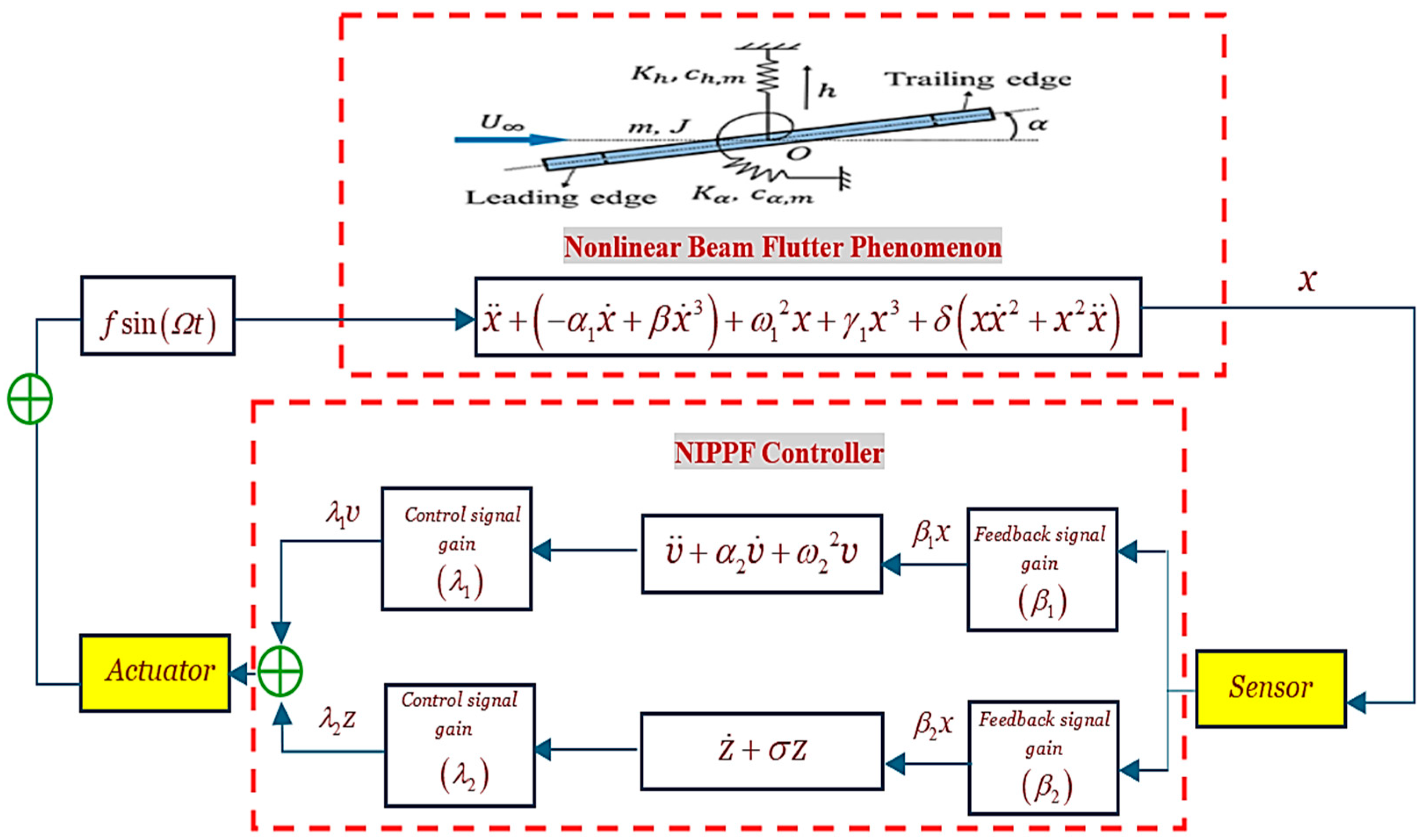
2.1. Uncontrolled System Dynamics

This segment outlines the mathematical model used to represent the flutter beam system. As illustrated in Figure 1, the structure is simplified and denoted as a one-degree-of-freedom system [2] for the purpose of this analysis.

$$\ddot{x}+\epsilon \left(-{\alpha }_1\dot{x}+\beta {\dot{x}}^3\right)+{{\omega }_1}^{2}x+\epsilon {\gamma }_1{x}^3+\epsilon \delta \left(x{\dot{x}}^2+x^2\ddot{x}\right)=\epsilon f\sin \left(\mathsf{\Omega }t\right),$$

(1)

2.2. System Dynamics with NIPPF Control

To analyze the behavior of flutter beams, engineers often employ simplified models like the one depicted in Figure 1, which represents a section of an aircraft structure. When an external force acts upon this system, a Nonlinear Integral Positive Position Feedback controller can be laboring to dampen the resulting vibrations. Equations (2)–(4) reflect the system’s behavior under these conditions, incorporating both the external force and the influence of the NIPPF controller.

$$\ddot{x}+\epsilon \left(-{\alpha }_1\dot{x}+\beta {\dot{x}}^3\right)+{{\omega }_1}^{2}x+\epsilon {\gamma }_1{x}^3+\epsilon \delta \left(x{\dot{x}}^2+x^2\ddot{x}\right)=\epsilon f\sin \left(\mathsf{\Omega }t\right)+\epsilon {\lambda }_{1}v+\epsilon {\lambda }_{2}z,$$

(2)

$$\ddot{v}+\epsilon {\alpha }_2\dot{v}+{{\omega }_2}^{2}v=\epsilon {\beta }_{1}x,$$

(3)

$$\dot{z}+\sigma z={\beta }_{2}x.$$

(4)

which can be illustrated in Figure 2 as a flowchart.

3. Analytical Investigations

3.1. Perturbation Analysis

This segment employs a multiple scale perturbation technique, as described in [29,30,31], to determine an approximate solution for the nonlinear dynamical system. This method allows for the derivation of a first-order approximate solution:

$$\begin{array}{l}x(t;\epsilon )=x_0(T_0,T_1)+\epsilon x_1(T_0,T_1)+O({\epsilon }^2),\\ v(t;\epsilon )=y_0(T_0,T_1)+\epsilon y_1(T_0,T_1)+O({\epsilon }^2),\\ z(t;\epsilon )=z_0(T_0,T_1)+\epsilon z_1(T_0,T_1)+O({\epsilon }^2).\end{array}\}$$

(5)

where, some place, the negligible agitation parameter $\epsilon$ is located at $0<\epsilon \ll 1$. Agreement states two time scales, $T_0$ and $T_1$, in which $T_0=t$ represents a fast scale, while $T_1=\epsilon t$ is the slow one. The derivatives of time are rehabilitated into

$$\begin{array}{l}{\displaystyle \frac{d}{dt}}=D_0+\epsilon D_1+{\epsilon }^2{D}_2+\dots ,\\ {\displaystyle \frac{d^2}{d{t}^2}}=D_0^2+2\epsilon D_0{D}_1+\dots ,\end{array}\} D_j={\displaystyle \frac{\partial }{\partial T_j}}(j=0,1).$$

(6)

Equations (5) and (6) should be inserted into Equations (2)–(4) so that:

$$\left({D_0}^2+{{\omega }_1}^2\right)x_0+\epsilon \left({D_0}^2+{{\omega }_1}^2\right)x_1=\epsilon \left(\begin{array}{l}f\sin \left(\mathsf{\Omega }t\right)+{\lambda }_1{v}_0+{\lambda }_2{z}_0-2D_0{D}_1{x}_0\\ +{\alpha }_1{D}_0{x}_0-{\gamma }_1{x_0}^3-\beta {\left(D_0{x}_0\right)}^3\\ -\delta \left(x_0{\left(D_0{x}_0\right)}^2+{x_0}^2{D_0}^2{x}_0\right)\end{array}\right)+O({\epsilon }^2),$$

(7)

$$\left({D_0}^2+{{\omega }_2}^2\right)v_0+\epsilon \left({D_0}^2+{{\omega }_2}^2\right)v_1=\epsilon \left({\beta }_1{x}_0-2D_0{D}_1{v}_0-{\alpha }_2{D}_0{v}_0\right)+O({\epsilon }^2),$$

(8)

$$\left(D_0+\sigma \right)z_0+\epsilon \left(D_0+\sigma \right)z_1={\beta }_2{x}_0+\epsilon \left({\beta }_2{x}_1-D_1{z}_0\right).$$

(9)

Connect the quantities of the equal power of $\epsilon$:

• $O({\epsilon }^0)$

  $$({D_0}^2+{{\omega }_1}^2)x_0=0,$$

  (10)

  $$\left({D_0}^2+{{\omega }_2}^2\right)v_0=0,$$

  (11)

  $$\left(D_0+\sigma \right)z_0={\beta }_2{x}_0.$$

  (12)
• $O(\epsilon )$

  $$\begin{array}{c}\left({D_0}^2+{{\omega }_1}^2\right)x_1=f\sin \left(\mathsf{\Omega }t\right)+{\lambda }_1{v}_0+{\lambda }_2{z}_0-2D_0{D}_1{x}_0+{\alpha }_1{D}_0{x}_0-{\gamma }_1{x_0}^3-\beta {\left(D_0{x}_0\right)}^3\\ -\delta \left(x_0{\left(D_0{x}_0\right)}^2+{x_0}^2{D_0}^2{x}_0\right)\end{array},$$

  (13)

  $$\left({D_0}^2+{{\omega }_2}^2\right)v_1={\beta }_1{x}_0-2D_0{D}_1{v}_0-{\alpha }_2{D}_0{v}_0,$$

  (14)

  $$\left(D_0+\sigma \right)z_1={\beta }_2{x}_1-D_1{z}_0.$$

  (15)

From Equations (10)–(12), cracking the standardized differential equations, we obtain:

$$x_0(T_0,T_1)=A(T_1)e^{i{\omega }_1{T}_0}+\overline{A}(T_1)e^{-i{\omega }_1{T}_0},$$

(16)

$$v_0(T_0,T_1)=B(T_1)e^{i{\omega }_2{T}_0}+\overline{B}(T_1)e^{-i{\omega }_2{T}_0},$$

(17)

$$z_0=\left({\displaystyle \frac{\sigma -i{\omega }_1}{{\sigma }^2+{{\omega }_1}^2}}\right)\left({\beta }_{2}A{e}^{i{\omega }_1{T}_0}+{\overline{\beta }}_{2}A{e}^{-i{\omega }_1{T}_0}\right).$$

(18)

Differential Equations (16)–(18) with respect to t are submitted in Equations (13)–(15):

$$\begin{array}{c}\left({D_0}^2+{{\omega }_1}^2\right)x_1={\displaystyle \frac{f}{2i}}{e}^{i\mathsf{\Omega }{T}_0}+{\lambda }_{1}B{e}^{i{\omega }_2{T}_0}+{\lambda }_2{\beta }_2\left({\displaystyle \frac{\sigma -i{\omega }_1}{{\sigma }^2+{{\omega }_1}^2}}\right)A{e}^{i{\omega }_1{T}_0}-2i{\omega }_{1}DA{e}^{i{\omega }_1{T}_0}\\ +\left({\alpha }_{1}i{\omega }_{1}A-3\beta i{{\omega }_1}^3{A}^2\overline{A}-3{\gamma }_1{A}^2\overline{A}+2\delta {{\omega }_1}^2{A}^2\overline{A}\right)A{e}^{i{\omega }_1{T}_0}+C.C.\end{array},$$

(19)

$$\left({D_0}^2+{{\omega }_2}^2\right)v_1={\beta }_{1}A{e}^{i{\omega }_1{T}_0}-2i{\omega }_{2}DB{e}^{i{\omega }_2{T}_0}-i{\alpha }_2{\omega }_{2}B{e}^{i{\omega }_2{T}_0}+C.C.$$

(20)

The complex conjugate components are gathered under the abbreviation C.C. After removing the secular terms, acquire the following forms:

$$\begin{array}{l}{\displaystyle \frac{f}{2i}}{e}^{i\mathsf{\Omega }{T}_0}+{\lambda }_{1}B{e}^{i{\omega }_2{T}_0}+{\lambda }_2{\beta }_2\left({\displaystyle \frac{\sigma -i{\omega }_1}{{\sigma }^2+{{\omega }_1}^2}}\right)A{e}^{i{\omega }_1{T}_0}-2i{\omega }_{1}DA{e}^{i{\omega }_1{T}_0}\\ +\left({\alpha }_{1}i{\omega }_{1}A-3\beta i{{\omega }_1}^3{A}^2\overline{A}-3{\gamma }_1{A}^2\overline{A}+2\delta {{\omega }_1}^2{A}^2\overline{A}\right)A{e}^{i{\omega }_1{T}_0}=0\end{array},$$

(21)

$$\left(-2i{\omega }_{2}DB-i{\alpha }_2{\omega }_{2}B\right)e^{i{\omega }_2{T}_0}+{\beta }_{1}A{e}^{i{\omega }_1{T}_0}=0.$$

(22)

Based on the first approximation, we deduced the subsequent resonances:

(i)

PR: $\mathsf{\Omega }\cong {\omega }_1$

(ii)

IR: ${\omega }_1={\omega }_2$

3.2. Periodic Solutions

In this part, for the chosen resonance case $\mathsf{\Omega }\cong {\omega }_1$ and ${\omega }_1={\omega }_2$, with the second hand to confer the solvability surroundings, we will familiarize the detuning parameters $({\sigma }_1)\&({\sigma }_2)$ so that:

$$\begin{array}{l}\mathsf{\Omega }={\omega }_1+\epsilon {\sigma }_1,\\ {\omega }_2={\omega }_1+\epsilon {\sigma }_2.\end{array}\}$$

(23)

Include Equation (23) in the secular and insignificant division terms in Equations (21) and (22) for compiling the solvability conditions as:

$$\begin{array}{l}-2i{\omega }_{1}DA+{\lambda }_2{\beta }_2\left({\displaystyle \frac{\sigma -i{\omega }_1}{{\sigma }^2+{{\omega }_1}^2}}\right)A+{\alpha }_{1}i{\omega }_{1}A-3\beta i{{\omega }_1}^3{A}^2\overline{A}\\ -3{\gamma }_1{A}^2\overline{A}+2\delta {{\omega }_1}^2{A}^2\overline{A}+{\displaystyle \frac{f}{2i}}{e}^{i{\sigma }_1{T}_1}+{\lambda }_{1}B{e}^{i{\sigma }_2{T}_1}=0\end{array},$$

(24)

$$-2i{\omega }_{2}DB-i{\alpha }_2{\omega }_{2}B+{\beta }_{1}A{e}^{-i{\sigma }_2{T}_1}=0.$$

(25)

To examine the resolution of (24) and (25), exchange $A$ and $B$ with the polar form as:

$$A(T_1)={\displaystyle \frac{1}{2}}{a}_1(T_1)e^{i{\theta }_1{T}_1},DA(T_1)={\displaystyle \frac{1}{2}}\left({\dot{a}}_1(T_1)+i{a}_1{\dot{\theta }}_1(T_1)\right)e^{i{\theta }_1{T}_1},$$

(26)

$$B(T_1)={\displaystyle \frac{1}{2}}{a}_2(T_1)e^{i{\theta }_2{T}_1},DB(T_1)={\displaystyle \frac{1}{2}}\left({\dot{a}}_2(T_1)+i{a}_2{\dot{\theta }}_2(T_1)\right)e^{i{\theta }_2{T}_1}.$$

(27)

where $a_1$ and $a_2$ are the steady-state amplitudes of the system and control motions, individually, and ${\varphi }_1\&{\varphi }_2$ are stated as the phases of the motion. The following amplitude–phase modulating equations are obtained by inserting (26) and (27) into (24) and (25):

$${\dot{a}}_1={\displaystyle \frac{1}{2}}{\alpha }_1{a}_1-{\displaystyle \frac{{\lambda }_2{\beta }_2{a}_1}{2\left({\sigma }^2+{{\omega }_1}^2\right)}}-{\displaystyle \frac{3}{8}}\beta {{\omega }_1}^2{a_1}^3-{\displaystyle \frac{f}{2{\omega }_1}}\cos {\varphi }_1+{\displaystyle \frac{{\lambda }_1}{2{\omega }_1}}{a}_2\sin {\varphi }_2,$$

(28)

$$a_1{\dot{\theta }}_1={\displaystyle \frac{3}{8{\omega }_1}}{\gamma }_1{a_1}^3-{\displaystyle \frac{1}{4}}\delta {\omega }_1{a_1}^3-{\displaystyle \frac{{\lambda }_2{\beta }_2\sigma a_1}{2{\omega }_1\left({\sigma }^2+{{\omega }_1}^2\right)}}-{\displaystyle \frac{f}{2{\omega }_1}}\sin {\varphi }_1-{\displaystyle \frac{{\lambda }_1}{2{\omega }_1}}{a}_2\cos {\varphi }_2,$$

(29)

$${\dot{a}}_2=-{\displaystyle \frac{1}{2}}{\alpha }_2{a}_2-{\displaystyle \frac{{\beta }_1}{2{\omega }_2}}{a}_1\sin {\varphi }_2,$$

(30)

$$a_2{\dot{\theta }}_2=-{\displaystyle \frac{{\beta }_1}{2{\omega }_2}}{a}_1\cos {\varphi }_2.$$

(31)

wherever ${\varphi }_1={\sigma }_1{T}_1-{\theta }_1$ and ${\varphi }_2={\sigma }_2{T}_1+{\theta }_2-{\theta }_1$. Referring to the primary system parameters, the succeeding equations exist:

$${\dot{a}}_1={\displaystyle \frac{1}{2}}{\alpha }_1{a}_1-{\displaystyle \frac{{\lambda }_2{\beta }_2{a}_1}{2\left({\sigma }^2+{{\omega }_1}^2\right)}}-{\displaystyle \frac{3}{8}}\beta {{\omega }_1}^2{a_1}^3-{\displaystyle \frac{f}{2{\omega }_1}}\cos {\varphi }_1+{\displaystyle \frac{{\lambda }_1}{2{\omega }_1}}{a}_2\sin {\varphi }_2,$$

(32)

$${\dot{\varphi }}_1={\sigma }_1-{\displaystyle \frac{3}{8{\omega }_1}}{\gamma }_1{a}_1^2+{\displaystyle \frac{1}{4}}\delta {\omega }_1{a}_1^2+{\displaystyle \frac{{\lambda }_2{\beta }_2\sigma }{2{\omega }_1\left({\sigma }^2+{{\omega }_1}^2\right)}}+{\displaystyle \frac{f}{2{\omega }_1{a}_1}}\sin {\varphi }_1+{\displaystyle \frac{{\lambda }_1}{2{\omega }_1{a}_1}}{a}_2\cos {\varphi }_2,$$

(33)

$${\dot{a}}_2=-{\displaystyle \frac{1}{2}}{\alpha }_2{a}_2-{\displaystyle \frac{{\beta }_1}{2{\omega }_2}}{a}_1\sin {\varphi }_2,$$

(34)

$${\dot{\varphi }}_2=({\sigma }_2-{\sigma }_1)+{\dot{\varphi }}_1-{\displaystyle \frac{{\beta }_1}{2a_2{\omega }_2}}{a}_1\cos {\varphi }_2.$$

(35)

By computing the equilibrium solutions of Equations (32)–(35) and analyzing their firmness as an occupation of the parameters (${\sigma }_1,{\sigma }_2,\sigma ,{\alpha }_1,{\alpha }_2,\beta ,{\beta }_1,{\beta }_2,{\gamma }_1,\delta$, and $f$), the effectiveness of the control law will be assessed.

3.3. Fixed-Point Solution

Equations (32) through (35) may have a fixed point for a steady-state solution that can be found by stroking ${\dot{a}}_1={\dot{a}}_2={\dot{\varphi }}_1={\dot{\varphi }}_2=0$

$${\displaystyle \frac{f}{2{\omega }_1}}\cos {\varphi }_1-{\displaystyle \frac{{\lambda }_1}{2{\omega }_1}}{a}_2\sin {\varphi }_2={\displaystyle \frac{1}{2}}{\alpha }_1{a}_1-{\displaystyle \frac{{\lambda }_2{\beta }_2{a}_1}{2\left({\sigma }^2+{{\omega }_1}^2\right)}}-{\displaystyle \frac{3}{8}}\beta {\omega }_1^2{a}_1^3,$$

(36)

$${\displaystyle \frac{f}{2{\omega }_1}}\sin {\varphi }_1+{\displaystyle \frac{{\lambda }_1}{2{\omega }_1}}{a}_2\cos {\varphi }_2={\displaystyle \frac{3}{8{\omega }_1}}{\gamma }_1{a}_1^3-{\sigma }_1{a}_1+{\displaystyle \frac{1}{4}}\delta {\omega }_1{a}_1^3-{\displaystyle \frac{{\lambda }_2{\beta }_2\sigma a_1}{2{\omega }_1\left({\sigma }^2+{\omega }_1^2\right)}},$$

(37)

$${\displaystyle \frac{{\beta }_1}{2{\omega }_2}}{a}_1\sin {\varphi }_2=-{\displaystyle \frac{1}{2}}{\alpha }_2{a}_2,$$

(38)

$${\displaystyle \frac{{\beta }_1}{2{\omega }_2}}{a}_1\cos {\varphi }_2=({\sigma }_2-{\sigma }_1)a_2.$$

(39)

Equations (38) and (39) can be squared and then both sides added to obtain the following equation:

$$\left(4{{\omega }_2}^2{\left({\sigma }_2-{\sigma }_1\right)}^2+{{\alpha }_2}^2{{\omega }_2}^2\right){a_2}^2={{\beta }_1}^2{a_1}^2.$$

(40)

From (38) and (39), we have:

$$\cos {\varphi }_2={\displaystyle \frac{2{\omega }_2\left({\sigma }_2-{\sigma }_1\right)a_2}{{\beta }_1{a}_1}},$$

(41)

$$\sin {\varphi }_2=-{\displaystyle \frac{{\omega }_2{\alpha }_2{a}_2}{{\beta }_1{a}_1}}.$$

(42)

Inserting (41) and (42) into (36) and (37), we obtain

$${\displaystyle \frac{f}{2{\omega }_1}}\cos {\varphi }_1={\displaystyle \frac{1}{2}}{\alpha }_1{a}_1-{\displaystyle \frac{{\lambda }_2{\beta }_2{a}_1}{2\left({\sigma }^2+{{\omega }_1}^2\right)}}-{\displaystyle \frac{3}{8}}\beta {\omega }_1^2{a}_1^3-{\displaystyle \frac{{\lambda }_1{\omega }_2{\alpha }_2{a}_2^2}{2{\omega }_1{\beta }_1{a}_1}},$$

(43)

$$\cos {\varphi }_1={\displaystyle \frac{2{\omega }_1}{f}}\left({\displaystyle \frac{1}{2}}{\alpha }_1{a}_1-{\displaystyle \frac{{\lambda }_2{\beta }_2{a}_1}{2\left({\sigma }^2+{\omega }_1^2\right)}}-{\displaystyle \frac{3}{8}}\beta {\omega }_1^2{a}_1^3-{\displaystyle \frac{{\lambda }_1{\omega }_2{\alpha }_2{a}_2^2}{2{\omega }_1{\beta }_1{a}_1}}\right),$$

(44)

$${\displaystyle \frac{f}{2{\omega }_1}}\sin {\varphi }_1={\displaystyle \frac{3}{8{\omega }_1}}{\gamma }_1{a}_1^3-{\sigma }_1{a}_1+{\displaystyle \frac{1}{4}}\delta {\omega }_1{a}_1^3-{\displaystyle \frac{{\lambda }_2{\beta }_2\sigma a_1}{2{\omega }_1\left({\sigma }^2+{\omega }_1^2\right)}}-{\displaystyle \frac{{\lambda }_1{\omega }_2\left({\sigma }_2-{\sigma }_1\right)a_2^2}{{\omega }_1{\beta }_1{a}_1}},$$

(45)

$$\sin {\varphi }_1={\displaystyle \frac{2{\omega }_1}{f}}\left({\displaystyle \frac{3}{8{\omega }_1}}{\gamma }_1{a}_1^3-{\sigma }_1{a}_1-{\displaystyle \frac{1}{4}}\delta {\omega }_1{a}_1^3-{\displaystyle \frac{{\lambda }_2{\beta }_2\sigma a_1}{2{\omega }_1\left({\sigma }^2+{\omega }_1^2\right)}}-{\displaystyle \frac{{\lambda }_1{\omega }_2\left({\sigma }_2-{\sigma }_1\right)a_2^2}{{\omega }_1{\beta }_1{a}_1}}\right).$$

(46)

Squaring and adding Equations (43) and (45), we obtain

$${\left(\begin{array}{l}{\displaystyle \frac{1}{2}}{\alpha }_1{a}_1-{\displaystyle \frac{{\lambda }_2{\beta }_2{a}_1}{2\left({\sigma }^2+{\omega }_1^2\right)}}\\ -{\displaystyle \frac{3}{8}}\beta {\omega }_1^2{a}_1^3-{\displaystyle \frac{{\lambda }_1{\omega }_2{\alpha }_2{a}_2^2}{2{\omega }_1{\beta }_1{a}_1}}\end{array}\right)}^2+{\left(\begin{array}{l}{\displaystyle \frac{3}{8{\omega }_1}}{\gamma }_1{a}_1^3-{\sigma }_1{a}_1-{\displaystyle \frac{1}{4}}\delta {\omega }_1{a}_1^3\\ -{\displaystyle \frac{{\lambda }_2{\beta }_2\sigma a_1}{2{\omega }_1\left({\sigma }^2+{\omega }_1^2\right)}}-{\displaystyle \frac{{\lambda }_1{\omega }_2\left({\sigma }_2-{\sigma }_1\right)a_2^2}{{\omega }_1{\beta }_1{a}_1}}\end{array}\right)}^2={\displaystyle \frac{f^2}{4{\omega }_1^2}}.$$

(47)

The frequency–response Equations (32) and (35) are utilized to describe the behavior of the system’s steady-state solutions in the reasonable case, i.e., ($a_1\ne 0, a_2\ne 0$).

3.4. Determining Stability by Linearizing the System

To determine the stability of the equilibrium solution, we analyzed the eigenvalues of the Jacobian matrix derived from the right-hand side of the equations. Asymptotic stability of an equilibrium solution corresponds to all eigenvalues having negative real parts. Contrarywise, we doubt slightly that the eigenvalue holds a positive actual part, and the corresponding equilibrium is unbalanced. Begin by following these steps to evolve the stability of the steady-state solution. To originate the stability principles, we essentially study the conduct of small deviations from the steady-state solutions $a_{10},a_{20},{\varphi }_{10}$, and ${\varphi }_{20}$. Therefore, we adopt that

$$\begin{array}{l}{a}_1=a_{11}+a_{10},a_2=a_{21}+a_{20},{\varphi }_1={\varphi }_{11}+{\varphi }_{10},{\varphi }_2={\varphi }_{21}+{\varphi }_{20},\\ {\dot{a}}_1={\dot{a}}_{11}, {\dot{a}}_2={\dot{a}}_{21}, {\dot{\varphi }}_1={\dot{\varphi }}_{11}, {\dot{\varphi }}_2={\dot{\varphi }}_{21}.\end{array}\}.$$

(48)

everywhere $a_{10},a_{20},{\varphi }_{10}$, and ${\varphi }_{20}$ satisfy (32) and (35) and $a_{11},a_{21},{\varphi }_{11}$, and ${\varphi }_{21}$ are perturbations which are expected to be slightly related to $a_{10},a_{20},{\varphi }_{10}$, and ${\varphi }_{20}$. Relieving (48) into (32)–(35), expanding for small $a_{11},a_{21},{\varphi }_{11}$, and ${\varphi }_{21}$, and possessing linear terms in $a_{11},a_{21},{\varphi }_{11}$, and ${\varphi }_{21}$, we obtain

$${\dot{a}}_{11}=r_{11}{a}_{11}+r_{12}{\varphi }_{11}+r_{13}{a}_{21}+r_{14}{\varphi }_{21},$$

(49)

$${\dot{\varphi }}_{11}=r_{21}{a}_{11}+r_{22}{\varphi }_{11}+r_{23}{a}_{21}+r_{24}{\varphi }_{21},$$

(50)

$${\dot{a}}_{21}=r_{31}{a}_{11}+r_{32}{\varphi }_{11}+r_{33}{a}_{21}+r_{34}{\varphi }_{21},$$

(51)

$${\dot{\varphi }}_{21}=r_{41}{a}_{11}+r_{42}{\varphi }_{11}+r_{43}{a}_{21}+r_{44}{\varphi }_{21}.$$

(52)

where $r_{ij},i=1,2,3,4$ and $j=1,2,3,4$ are provided in the Appendix A.

Equations (49)–(52) can be presented in the resulting matrix:

$${\left[{\dot{a}}_{11}\hspace{1em}{\dot{\varphi }}_{11}\hspace{1em}{\dot{a}}_{21}\hspace{1em}{\dot{\varphi }}_{21}\right]}^T=\left[J\right]{\left[a_{11}\hspace{1em}{\varphi }_{11}\hspace{1em}{a}_{21}\hspace{1em}{\varphi }_{21}\right]}^T,$$

(53)

$$\left[J\right]=\left[\begin{array}{l}{\mathrm{r}}_{11}{ \mathrm{r}}_{12}{ \mathrm{r}}_{13}{ \mathrm{r}}_{14}\\ {\mathrm{r}}_{21}{ \mathrm{r}}_{22}{ \mathrm{r}}_{23}{ \mathrm{r}}_{24}\\ {\mathrm{r}}_{31}{ \mathrm{r}}_{32}{ \mathrm{r}}_{33}{ \mathrm{r}}_{34}\\ {\mathrm{r}}_{41}{ \mathrm{r}}_{42}{ \mathrm{r}}_{43}{ \mathrm{r}}_{44}\end{array}\right].$$

(54)

$\left[J\right]$ is the Jacobian matrix.

The eigenvalues of the Jacobian matrix govern the stability of the steady-state solutions. This leads to the following eigenvalue equation:

$$\left|\begin{array}{cccc}{r}_{11}-\beta & r_{12}& r_{13}& r_{14}\\ r_{21}& r_{22}-\beta & r_{23}& r_{24}\\ r_{31}& r_{32}& r_{33}-\beta & r_{34}\\ r_{41}& r_{42}& r_{43}& r_{44}-\beta \end{array}\right|=0.$$

(55)

wherever the following polynomial’s roots are located:

$${\beta }^4+{\mathsf{\Gamma }}_1{\beta }^3+{\mathsf{\Gamma }}_2{\beta }^2+{\mathsf{\Gamma }}_3\beta +{\mathsf{\Gamma }}_4=0.$$

(56)

The coefficients of Equation (54) $\left({\mathsf{\Gamma }}_i;i=1,\dots ,4\right)$ are labeled in the Appendix. The Routh–Hurwitz criterion can essentially be met for the resolution to the aforementioned system to be stable, meaning that:

$${\mathsf{\Gamma }}_1>0,{\mathsf{\Gamma }}_1{\mathsf{\Gamma }}_2-{\mathsf{\Gamma }}_3>0,{\mathsf{\Gamma }}_3({\mathsf{\Gamma }}_1{\mathsf{\Gamma }}_2-{\mathsf{\Gamma }}_3)-{\mathsf{\Gamma }}_1^2{\mathsf{\Gamma }}_4>0,{\mathsf{\Gamma }}_4>0.$$

(57)

4. Results and Discussion

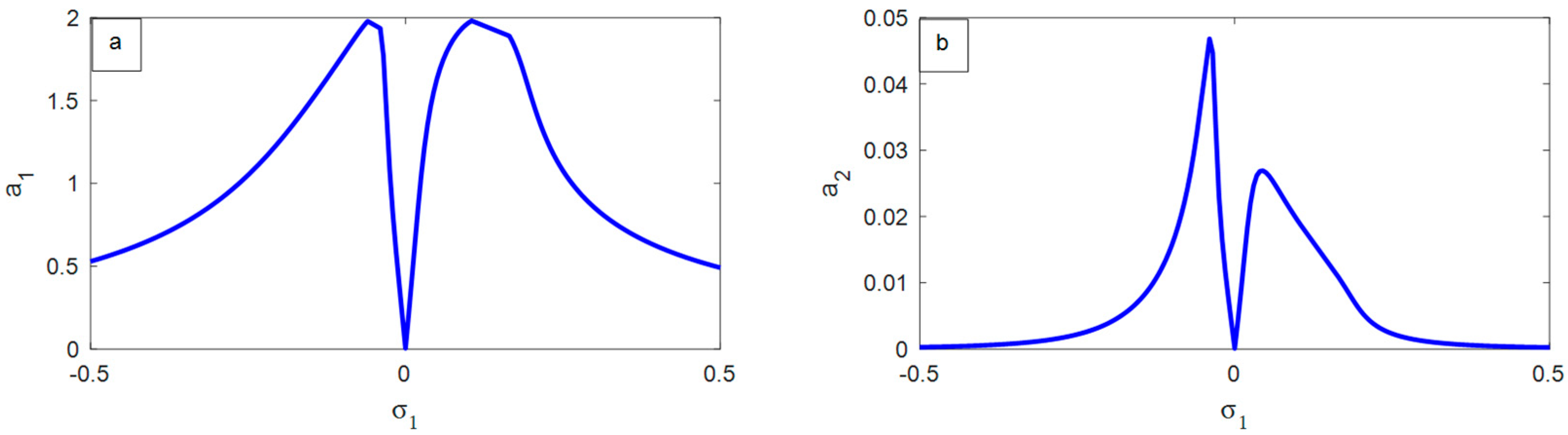
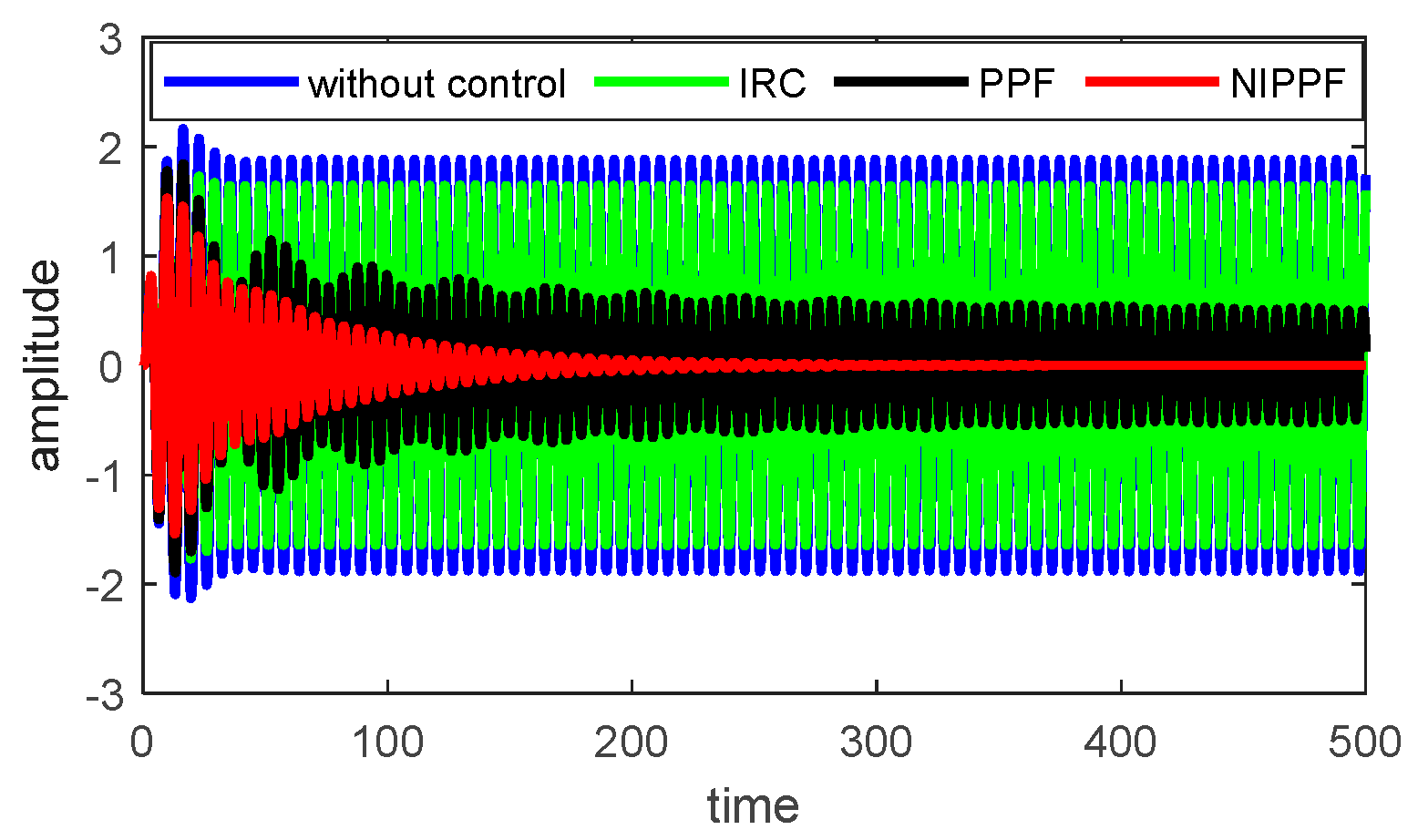
4.1. System Performance with and without NIPPF Control

To scrutinize the performance of the dynamical system, the fourth-order Runge–Kutta procedure (ode45 in MATLAB) [30] is pragmatic to invent the numerical solution of the particular non-control system in Equations (2)–(4). Our study’s primary focus was on the stability of a system that included the flutter spectacle in a forced and self-excited nonlinear beam. The graphical representation of the results includes plots of steady-state amplitudes versus detuning parameters, with figures generated using the specified values for the system parameters.

$$\left(\begin{array}{l}{\gamma }_1=0.2;\beta =0.05;{\beta }_1=0.001;{\beta }_2=0.005;{\alpha }_1=0.001;{\alpha }_2=0.0002;f=0.5;\delta =0.2;\\ {\lambda }_1=25;{\lambda }_2=25;\sigma =0.5;{\sigma }_2=0;{\omega }_1={\omega }_2=1.\end{array}\right)$$

Figure 3 displays the basic system steady-state amplitudes, previously adding NIPPF controllers at the worst resonance case, which is about 1.93. After adding NIPPF controllers, the system amplitudes have decreased to extend by 0.004. This implies that the proficiency of the NIPPF controllers is around E_a. = 482.5 and vibrations are reduced by approximately 99.8% from their value without control.

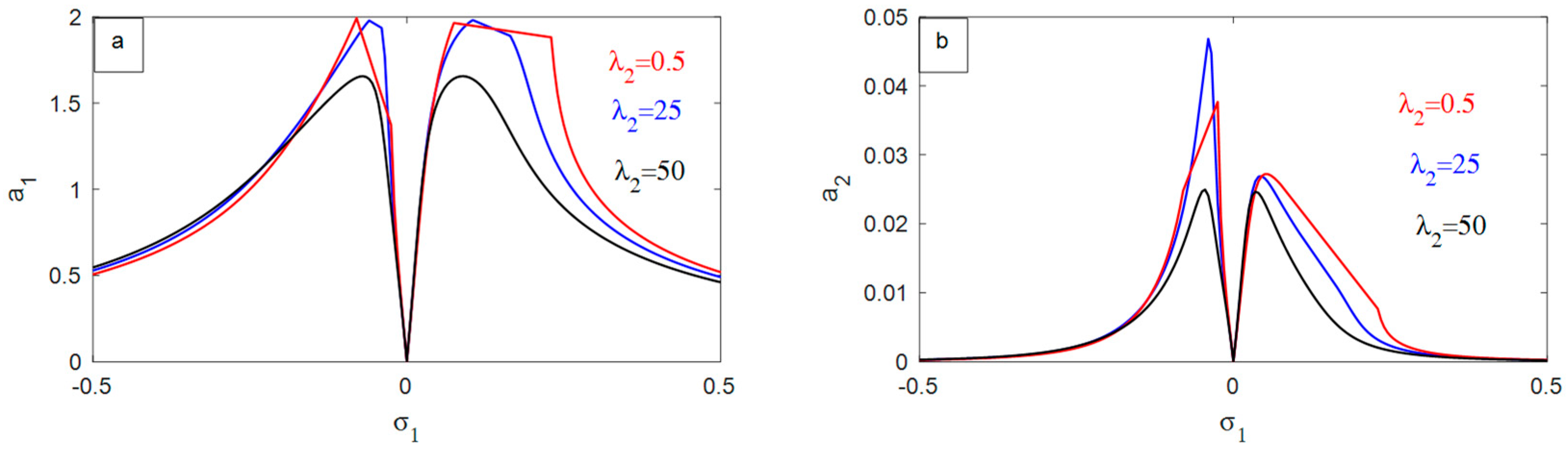
4.2. Occurrence Rejoinder Curvatures (ORC)

The rejoinder largeness is determined by both the detuning parameters ${\sigma }_1,{\sigma }_2$, and the excitation amplitude $f$. Equations (32) and (35) are resolved numerically and graphically to take the solution for the system and the NIPPF amplitudes. This graphical solution is derived concerning the detuning parameter ${\sigma }_1,{\sigma }_2$, providing a visual representation of how the amplitudes of these systems vary with changes in the detuning parameter ${\sigma }_1,{\sigma }_2$; two peaks are used to indicate this. Figure 4, Figure 5, Figure 6, Figure 7, Figure 8, Figure 9, Figure 10, Figure 11, Figure 12, Figure 13, Figure 14, Figure 15 and Figure 16 illustrate that the amplitude of the frequency–response curves can be asymmetrical at certain times. However, adjusting the values of various parameters can help improve the symmetry.

The frequency–response curves described in Figure 4 display the appearances of the focal structure and the NIPPF controller. The stable solutions, stated as solid lines, represent the controlled system’s frequency–response. Figure 4a illustrates the frequency–response curves of the focal structure, while Figure 4b displays the frequency–response bends of the supervisor. These graphs enable a pictorial assessment in the way the structures respond across different rates and highlight the stability areas indicated by the dense shapes. We can determine from this grid that the primary system amplitude’s smallest value is reached at ${\sigma }_1=0$, implying that the NIPPF controller is capable of suppressing focal structure vibrations in the situation of the primary resonance case. The generosities of both the focal structure and the NIPPF controller grow when the value of a harmonic excitation force increases, the jump phenomenon happens, and the smallest possible value of the focal structure amplitude happens at ${\sigma }_1=0$, as illustrated in Figure 5a,b.

The control signal gain ${\lambda }_1$ is represented in Figure 6a,b. We are providing a set of findings and observations regarding the influence of the NIPPF controller and its parameters on structure performance. The breadth of the swing to the right of the NIPPF controller indicates an extension in the control signal’s bandwidth, as illustrated in Figure 6a. Figure 6b shows that the fullness of the NIPPF controller drops monotonically, which is consistent with the desired objective of the control signal gain.

In Figure 7a,b, when the control signal gain ${\lambda }_2$ is increased, the focal structure amplitude and corresponding controller amplitude drop. Moreover, in Figure 8a,b, the vibration suppression bandwidth for the curves that simulate the amplitude of the focal structure and the associated controller around ${\sigma }_2=0$ are increasing when the feedback signal gain ${\beta }_1$ is increasing. Also, the amplitude of the system is decreased, as shown in Figure 8a, and the amplitude of the controller is increased, as shown in Figure 8b.

Figure 9a,b depict the impact of feedback signal gain ${\beta }_2$ on the frequency–response curves for the controller and focal structure, respectively. In Figure 9a, increasing the reaction signal decreases the vibration-lessening occurrence. In Figure 9b, advanced values of the feedback signal ${\beta }_2$ lead to decreased controller amplitudes.

Figure 10 illustrates how the controller’s damping factor affects both the focal structure and its frequency–response curve. Figure 10 expresses that, as ${\alpha }_2$ inflates, the regulator’s effectiveness in removing primary tone inflammations is reduced slightly, although the peak amplitudes of both the focal structure and the controller decline. As shown in Figure 11a,b, and Figure 12a,b, when increasing the values of nonlinear parameters $\beta$ and ${\gamma }_1$, the vibration amplitude of the system and the controller decreases.

Figure 13 shows that the effect of nonlinear parameters causes an increase in the efficiency of parameter $\delta$ where the vibration-lessening frequency is decreased. Figure 14 displays that once the efficiency of the linear parameter $\sigma$ becomes higher, the vibration discount frequency is shifted to the left.

For minor values of ordinary frequency for ${\sigma }_2=0$, i.e., (${\omega }_1={\omega }_2$), the peak amplitudes of the focal structure and the NIPPF controller grow, as does the bandwidth of the vibration reduction, so that in the event of a low natural frequency, the NIPPF controller is highly acceptable, as illustrated in Figure 15. We choose three different values of ${\sigma }_2$, and the amplitude of the focal structure realizes its slight value, as realized in Figure 16, when ${\sigma }_1={\sigma }_2$, which means that the NIPPF controller is more effective in the resonance situation.

5. Comparison

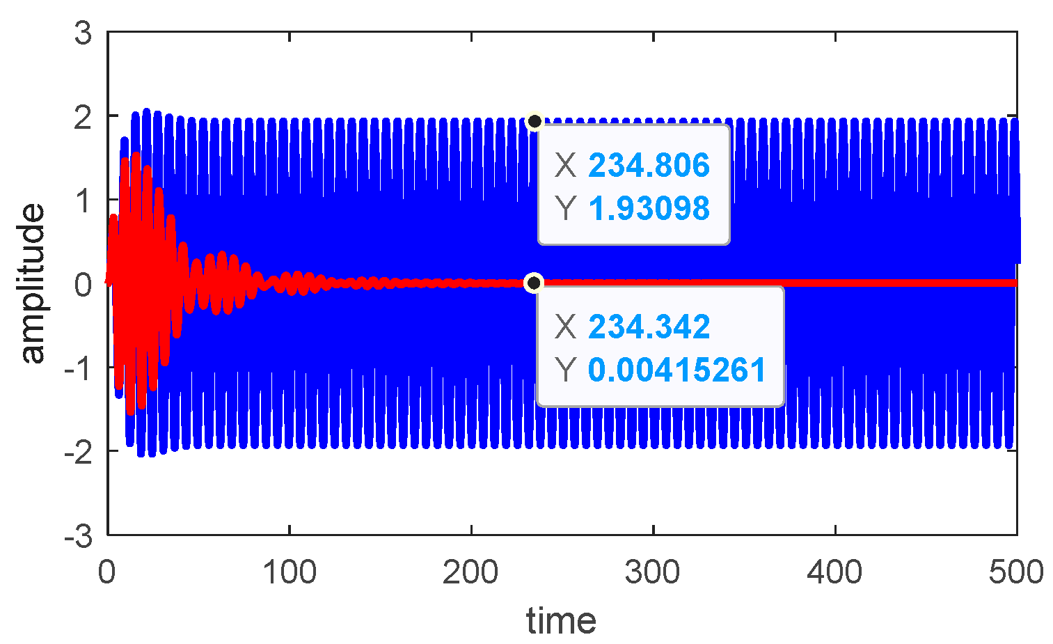
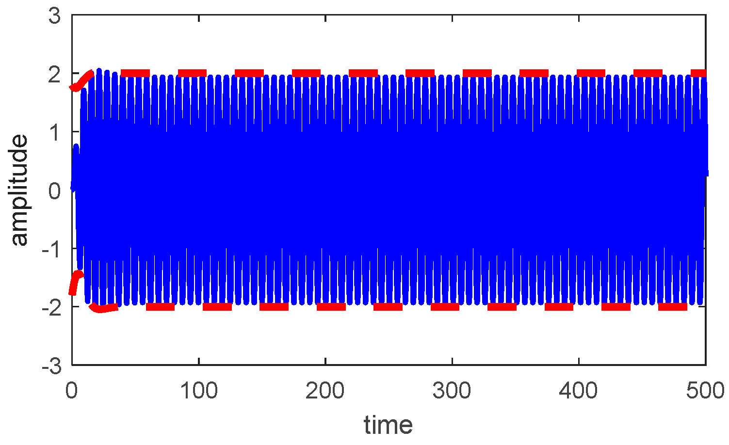
5.1. Comparison between Time History before and after the Controller

The NIPPF controller is the best way to reduce the focal structure’s amplitude, based on Figure 17. We are also pointing out the close alignment among geometric recreations and estimated resolutions for the uninhibited structure and the structure with the NIPPF supervisor.

5.2. Comparison between Perturbation Solution and Numerical Simulation

Figure 18 and Figure 19 illustrate the close agreement between the numerical and approximate solutions for both the uncontrolled and controlled systems, respectively. This strong correlation validates the reliability of both approaches in accurately representing the system’s behavior. Notably, Figure 19 highlights the effectiveness of the NIPPF controller, as demonstrated by the close alignment between the numerical and approximate solutions when the controller is implemented. These findings underscore the robustness of both the numerical and approximate methods in analyzing system dynamics across various control scenarios as presented in

Table 1. Comparison of some obtained approximate and numerical solutions.

Time	Approximate Solution beforeNIPPF	Numerical Solution beforeNIPPF
62.8	−1.9	−1.9
883.883	−1.9	−1.9
49.6	1.9	1.9
833.416	1.9	1.9
Time	Approximate Solution after NIPPF	Numerical Solution after NIPPF
62.8	−0.004	−0.004
883.883	−0.004	−0.004
49.6	0.004	0.004
833.416	0.004	0.004

.

5.3. Comparison with Previous Work

In Ref. [2], both the saturation controller and the velocity feedback controller were employed by the control algorithm. In addition to the saturation controller, the velocity feedback controller improves system damping without sacrificing controller efficiency. This, in turn, mitigates the impact of self-excitation, minimizes transient vibrations, and extends the system’s time margin. Our conclusions are the best combinations of time margins, steady solution zones, and controller parameters given the expected external excitation bandwidth. We have used the NIPPF controller in the system in this paper. Subsequently, studying the time antiquity and changed constraints before and after adding the supervisor, the vibration of the system is reduced after the controller feedback is added and the controller Ea is nearly 487. The amplitude of the exciting system has been lowered to approximately 99% compared to its value without control. There is also a high level of arrangement between the numerical and approximation resolutions.

6. Conclusions

This article addresses the challenge of controlling nonlinear vibrations in a flutter beam system. The authors introduce a novel approach using an NIPPF controller to mitigate the system’s lateral vibrations. The mathematical model, encompassing both the system and the controller, is represented by two second-order nonlinear differential equations coupled with first-order linear differential equations.

The study employs asymptotic analysis to derive an approximate solution for this nonlinear model. Frequency response diagrams are generated, and a comprehensive sensitivity analysis is conducted to examine the influence of various system and controller parameters. The Routh–Hurwitz criterion is utilized to assess the stability of the system.

Numerical simulations validate the analytical findings, confirming the accuracy of the frequency response curves. Adjusting the values of most parameters resulted in enhanced symmetry of the amplitudes in the frequency response curves. The main points from the preceding discussion can be summarized as follows:

• The Nonlinear Integral Positive Position Feedback (NIPPF) controller effectively mitigates high-amplitude atmospheres inside nonlinear structures.
• The PR and IR case $\mathsf{\Omega }\cong {\omega }_1$ and ${\omega }_2={\omega }_1$ is one of the worst vibrating reverberation cases.
• The breadth of the exciting structure declined around 99.8% after employing the NIPPF reaction supervisor associated with its rate deprived of the regulator.
• The efficiency of the NIPPF reaction supervisor, signified as Ea, influences approximately 482.5, showcasing its high effectiveness in supervising the structure’s performance.
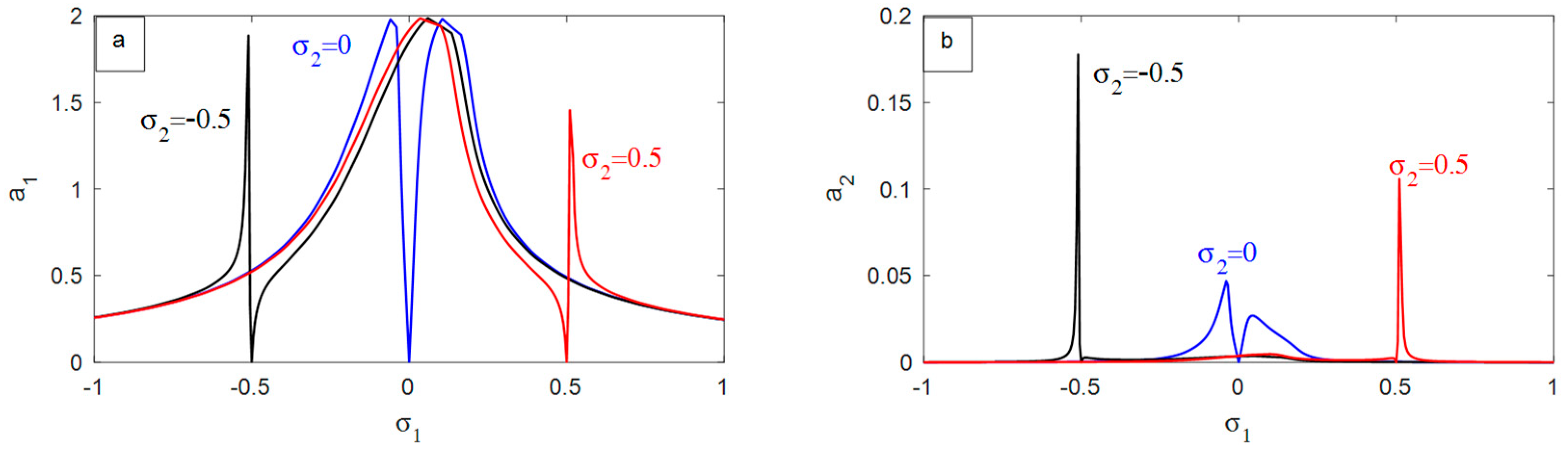
• The comeback or performance of the measured structure deepens with the increase in the peripheral excitement force, $f$.
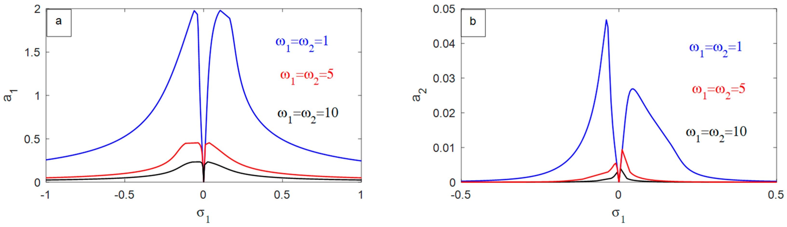
• The rejoinder of the focal structure diminished with the growth of the natural frequency ${\omega }_1$.
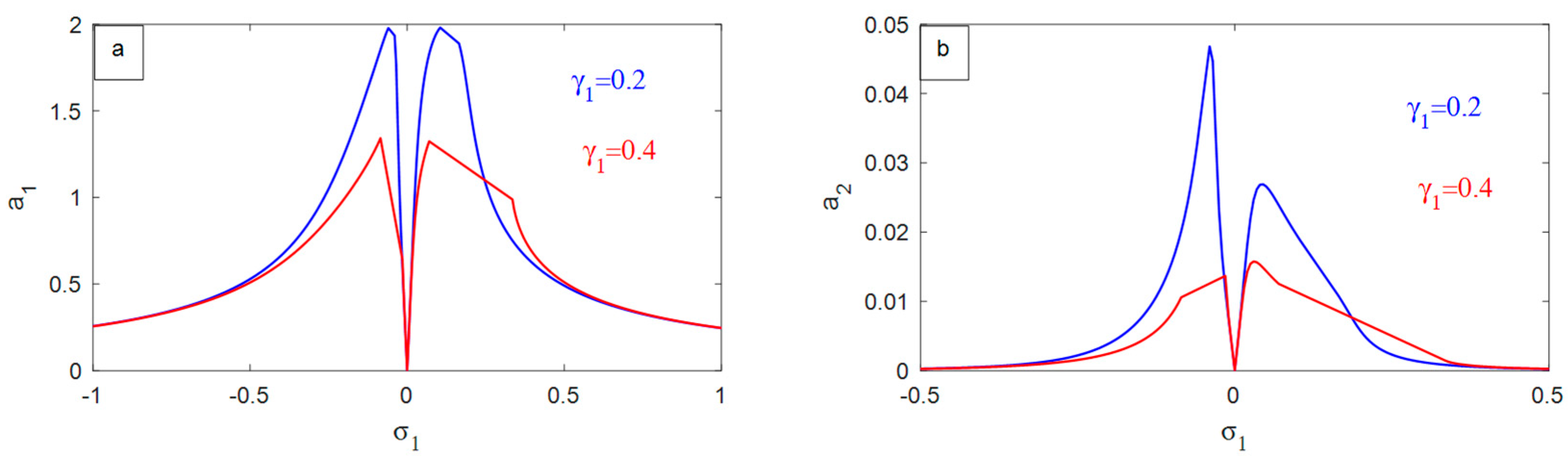
• Increasing the NIPPF parameter ${\lambda }_1$ shifts the curves to the right, which can improve the performance of the NIPPF controller, particularly in mitigating high-amplitude vibrations within the nonlinear system, which is beneficial to the operation of the NIPPF controller.
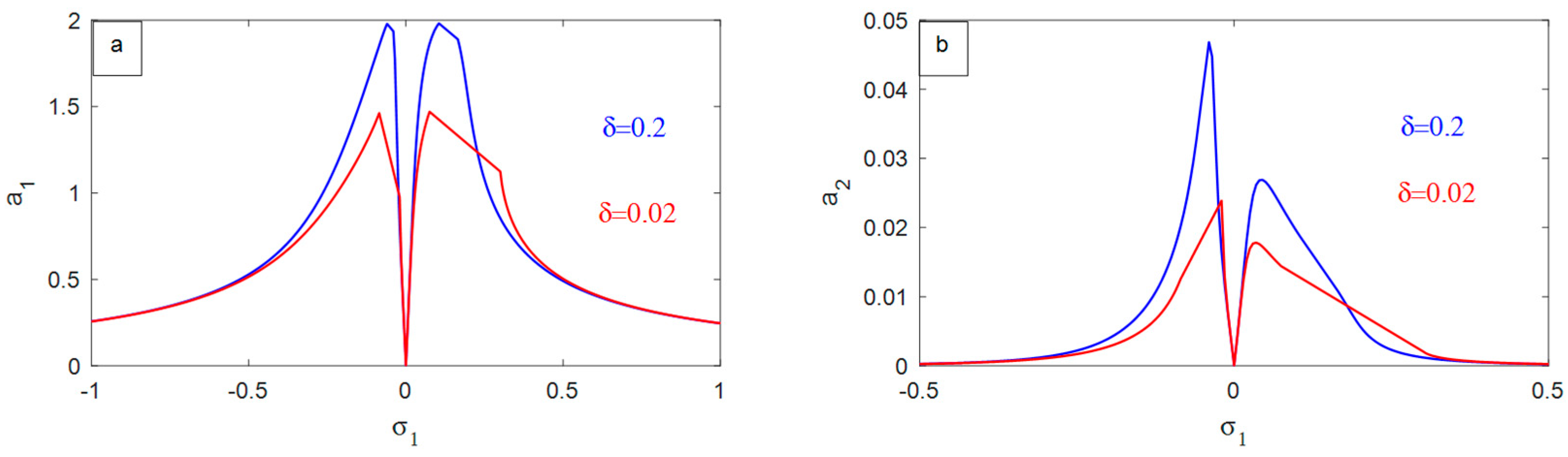
• For the NIPPF parameter, the amplitude of the measured system decreases very sluggishly.
• The smallest possible amplitudes of the vibrating suspended cable happen when ${\sigma }_1={\sigma }_2$
• The frequency response curves and the Runge–Kutta fourth-order method yield consistent results, validating the analysis in both the frequency and time domains.
• The closed-loop response of the relative displacement, using the NIPPF controller, exhibits a peak overshoot, which is a characteristic of the system’s transient behavior.
• The modified NIPPF controller effectively controls the relative displacement of the suspension system. This is evident in the improved closed-loop performance, characterized by minimized peak overshoot and settling time.

References

- Warminski, J.; Cartmell, M.P.; Mitura, A.; Bochenski, M. Active vibration control of a nonlinear beam with self-and external excitations. Shock Vib. 2013, 20, 1033–1047. [Google Scholar] [CrossRef]
- Abdelhafez, H.M.; Nasedkin, A.V.; Nassar, M.E. Elimination of the Flutter Phenomenon in a Forced and Self-excited Nonlinear Beam Using an Improved Saturation Controller Algorithm. In Nonlinear Wave Dynamics of Materials and Structures. Advanced Structured Materials; Altenbach, H., Eremeyev, V., Pavlov, I., Porubov, A., Eds.; Springer: Cham, Switzerland, 2020. [Google Scholar]
- Abadi, A. Nonlinear Dynamics of Self-Excitation in Autoparametric Systems. Ph.D. Thesis, University of Utrecht, Utrecht, The Netherlands, 2003. [Google Scholar]
- Nayfeh, A.H.; Mook, D.T. Nonlinear Oscillations; John Wiley & Sons: New York, NY, USA, 1995. [Google Scholar]
- Saeed, N.A.; Eissa, M. Nonlinear time delay saturation-based controller for suppression of nonlinear beam vibrations. Appl. Math. Model 2013, 37, 8846–8864. [Google Scholar] [CrossRef]
- Li, W.; Laima, S. Experimental Investigations on Nonlinear Flutter Behaviors of a Bridge Deck with Different Leading and Trailing Edges. Appl. Sci. 2020, 10, 7781. [Google Scholar] [CrossRef]
- An, X.; Li, S.; Wu, T. Modeling Nonlinear Aeroelastic Forces for Bridge Decks with Various Leading Edges Using LSTM Networks. Appl. Sci. 2023, 13, 6005. [Google Scholar] [CrossRef]
- Omidi, E.; Nima Mahmoodi, S. Multimode modified positive position feedback to control a collocated structure. J. Dyn. Syst. Meas. Control 2015, 137, 051003. [Google Scholar] [CrossRef]
- Bauomy, H.S.; El-Sayed, A.T. Outcome of special vibration controller techniques linked to a cracked beam. Appl. Math. Model 2018, 37, 266–287. [Google Scholar]
- Jun, L. Positive position feedback control for high-amplitude vibration of a flexible beam to a principal resonance excitation. Shock Vib. 2010, 17, 187–203. [Google Scholar] [CrossRef]
- Amer, Y.A.; El-Sayed, A.T.; Abdel-Wahab, A.M.; Salman, H.F. Positive position feedback controller for nonlinear beam subject to harmonically excitation. Asian Res. J. Math. 2019, 12, 1–19. [Google Scholar] [CrossRef]
- Zhu, Q.; Yue, J.Z.; Liu, W.Q.; Wang, X.D.; Chen, J.; Hu, G.D. Active vibration control for piezoelectricity cantilever beam: An adaptive feedforward control method. Smart Mater. Struct. 2017, 26, 047003. [Google Scholar] [CrossRef]
- Das, A.S.; Dutt, J.K.; Ray, K. Active control of coupled flexural-torsional vibration in a flexible rotor–bearing system using electromagnetic actuator. Int. J. Non-Linear Mech. 2011, 46, 1093–1109. [Google Scholar] [CrossRef]
- Fuller, C.C.; Elliott, S.; Nelson, P.A. Active Control of Vibration; Academic Press: New York, NY, USA, 1996. [Google Scholar]
- El-Ganaini, W.A.; Saeed, N.A.; Eissa, M. Positive position feedback (PPF) controller for suppression of nonlinear system vibration. Nonlinear Dyn. 2013, 72, 517–537. [Google Scholar] [CrossRef]
- Saeed, N.A.; Awrejcewicz, J.; Elashmawey, R.A.; El-Ganaini, W.A.; Hou, L.; Sharaf, M. On 1/2-DOF active dampers to suppress multistability vibration of a 2-DOF rotor model subjected to simultaneous multiparametric and external harmonic excitations. Nonlinear Dyn. 2024, 112, 12061–12094. [Google Scholar] [CrossRef]
- Fyrillas, M.M.; Szeri, A.J. Control of ultra-and subharmonic resonances. J. Nonlinear Sci. 1998, 8, 131–159. [Google Scholar] [CrossRef]
- Fischer, A.; Eberhard, P. Controlling vibrations of a cutting process using predictive control. Comput. Mech. 2014, 54, 21–31. [Google Scholar] [CrossRef]
- Alluhydan, K.; Moatimid, G.M.; Amer, T.S.; Galal, A.A. Inspection of a Time-Delayed Excited Damping Duffing Oscillator. Axioms 2024, 13, 416. [Google Scholar] [CrossRef]
- Abdelhafez, H.; Nassar, M. Suppression of vibrations of a forced and self-excited nonlinear beam by using positive position feedback controller PPF. Br. J. Math. Comput. Sci. 2016, 17, 1–19. [Google Scholar] [CrossRef]
- Kandil, A.; Hamed, Y.S.; Alsharif, A.M. Rotor active magnetic bearings system control via a tuned nonlinear saturation oscillator. IEEE Access 2021, 9, 133694–133709. [Google Scholar] [CrossRef]
- Bauomy, H. Safety action over oscillations of a beam excited by moving load via a new active vibration controller. Math. Biosci. Eng. 2023, 20, 5135–5158. [Google Scholar] [CrossRef]
- Saeed, N.A.; Awrejcewicz, J.; Hafez, S.T.; Hou, L.; Aboudaif, M.K. Stability, bifurcation, and vibration control of a discontinuous nonlinear rotor model under rub-impact effect. Nonlinear Dyn. 2023, 111, 20661–20697. [Google Scholar] [CrossRef]
- Elashmawey, R.A.; Saeed, N.A.; Elganini, W.A.; Sharaf, M. An asymmetric rotor model under external, parametric, and mixed excitations: Nonlinear bifurcation, active control, and rub-impact effect. J. Low Freq. Noise Vib. Act. Control. 2024. [Google Scholar] [CrossRef]
- Jamshidi, R.; Collette, C. Optimal negative derivative feedback controller design for collocated systems based on H2 and H∞ method. Mech. Syst. Signal Process. 2022, 181, 109497. [Google Scholar] [CrossRef]
- Ren, Y.; Ma, W. Dynamic Analysis and PD Control in a 12-Pole Active Magnetic Bearing System. Mathematics 2024, 12, 2331. [Google Scholar] [CrossRef]
- Amer, Y.A.; Abd EL-Salam, M.N.; EL-Sayed, M.A. Behavior of a Hybrid Rayleigh-Van der Pol-Duffing Oscillator with a PD Controller. J. Appl. Res. Technol. 2022, 20, 58–67. [Google Scholar]
- Hamed, Y.S.; Alotaibi, H.; El-Zahar, E.R. Nonlinear vibrations analysis and dynamic responses of a vertical conveyor system controlled by a proportional derivative controller. IEEE Access 2020, 8, 119082–119093. [Google Scholar] [CrossRef]
- Kevorkian, J.; Cole, J.D. The method of multiple scales for ordinary differential equations. In Applied Mathematical Sciences; Springer: New York, NY, USA, 1996; Volume 114. [Google Scholar]
- Nayfeh, A.H. Perturbation Methods; John Wiley & Sons: New York, NY, USA, 1973. [Google Scholar]
- Dukkipati, R.V. Solving Vibration Analysis Problems Using MATLAB; New Age International Pvt Ltd. Publishers: New Delhi, India, 2007. [Google Scholar]