Comparative Study of Crossover Mathematical Model of Breast Cancer Based on Ψ-Caputo Derivative and Mittag-Leffler Laws: Numerical Treatments

Abstract

Two novel crossover models for breast cancer that incorporate $\Psi$-Caputo fractal variable-order fractional derivatives, fractal fractional-order derivatives, and variable-order fractional stochastic derivatives driven by variable-order fractional Brownian motion and the crossover model for breast cancer that incorporates Atangana–Baleanu Caputo fractal variable-order fractional derivatives, fractal fractional-order derivatives, and variable-order fractional stochastic derivatives driven by variable-order fractional Brownian motion are presented here, where we used a simple nonstandard kernel function $\Psi \left(t\right)$ in the first model and a non-singular kernel in the second model. Moreover, we evaluated our models using actual statistics from Saudi Arabia. To ensure consistency with the physical model problem, the symmetry parameter $\zeta$ is introduced. We can obtain the fractal variable-order fractional Caputo and Caputo–Katugampola derivatives as special cases from the proposed $\Psi$-Caputo derivative. The crossover dynamics models define three alternative models: fractal variable-order fractional model, fractal fractional-order model, and variable-order fractional stochastic model over three-time intervals. The stability of the proposed model is analyzed. The $\Psi$-nonstandard finite-difference method is designed to solve fractal variable-order fractional and fractal fractional models, and the Toufik–Atangana method is used to solve the second crossover model with the non-singular kernel. Also, the nonstandard modified Euler–Maruyama method is used to study the variable-order fractional stochastic model. Numerous numerical tests and comparisons with real data were conducted to validate the methods’ efficacy and support the theoretical conclusions.

1. Introduction

Breast cancer is a type of cancer that starts in breast cells. Breast cancer often originates from the epithelial lining of milk ducts or from within the lobules that generate milk. It is possible for a malignant tumor to expand to encompass additional bodily areas [1]. A person with breast cancer may have localized malignant cells in one or more breast regions; these are frequently palpable masses. It is possible for cancer to spread in either one or both breasts. On rare occasions, breast cancer spreads to other parts of the body, including the liver, skeleton, etc. Breast cancer is the second most common type of cancer globally, affecting women globally after lung cancer [2].

Physicians use a variety of strategies to treat cancer to either destroy cancer cells or stop them from proliferating. Strong medications are used in chemotherapy treatments to destroy aberrant cells, but these treatments have negative effects on the patient’s heart, a condition known as cardiotoxicity [3].

Scientists and researchers have proposed many theoretical and mathematical studies to investigate breast cancer dynamics [3,4,5,6,7,8]. For instance, the authors in [4] formulated a mathematical model to understand breast cancer in the population of Saudi Arabia. This study intended to reduce the number of cardiotoxic patients and raise the number of patients who recover following chemotherapy, which will aid in public health decision-making. In [3], the authors formulated the dynamics of cancer in the breast with adverse reactions of chemotherapy treatment on the heart of a patient in the fractional framework to visualize its dynamic behavior. Also, the authors in [8] developed, analyzed and simulated fractional mathematical models to investigate the transmission dynamics of different phases of breast cancer. The suggested breast cancer model incorporates three often-used fractional operators in epidemiology: Caputo, Caputo–Fabrizio, and Atangana–Baleanu Caputo operators.

Recent studies revealed that traditional fractional- or integer-order equations are less accurate than differential equations incorporating piecewise equations. Piecewise derivatives and fractional calculus’ short memory idea are comparable. A number of worthwhile studies were recently released (see [9,10,11]).

The generalized $\Psi$-Caputo operator is a flexible fractional derivative that provides a logical framework for dealing with a wide range of practical problems, where we can obtain the Caputo, Caputo–Katugampola, and Caputo–Hadamard derivatives as special cases from the proposed derivative. It has been successfully applied in many scientific domains, such as engineering, physics, and mathematical modeling [12,13,14]. Its versatility allows us to address complex systems and phenomena in a unified manner. For additional information, see [13]. It is particularly helpful for simulating systems that display memory effects and nonlocal behavior.

These days, engineering and science use the Caputo, Caputo–Fabrizio (CF), and Atangana–Baleanu (AB) fractional and fractal fractional operators extensively for modeling issues [15,16,17,18,19,20,21,22,23]. These operators are used by researchers worldwide to solve a wide range of issues. Real-world issues with actual data are of interest to scientists because they can be fitted with models to forecast the dynamics of a phenomenon in the future. These actual settings might be more suitable for future results than previously thought.

In this study, we will combine piecewise differential equations with the $\Psi$-Caputo fractal fractional-order and fractal variable-order fractional derivatives with variable-order fractional stochastic derivatives driven by the variable-order fractional Brownian motion derivative to form a new system for breast cancer that is presented for the first time in this paper. Moreover, we will present a second crossover model with a non-singular kernel, where the second crossover model for breast cancer that incorporates Atangana–Baleanu Caputo fractal variable-order fractional derivatives, fractal fractional-order derivatives, and variable-order fractional stochastic derivatives driven by variable-order fractional Brownian motion. We will discuss the stability study of this system. Moreover, we will develop numerical methods called the $\Psi$-nonstandard finite-difference method ($\Psi$-NSFDM) and the nonstandard modified Euler–Maruyama method (NMEMM) to study the behavior of the resulting solutions. Also, we will use the Toufik–Atangana (TAM) method to solve the second crossover model with a non-singular kernel. We will compare the results obtained with real data from the Kingdom of Saudi Arabia from 2014 to 2016. The proposed crossover models will be defined in three time periods, where the fractal fractional-order system will be studied in the first period, the fractal variable-order fractional system will be studied in the second period, and the variable-order fractional stochastic system will be studied in the third period. We will present several numerical simulations for different values of the nonstandard $\Psi \left(t\right)$ function, as well as fractional and fractal variable-order fractional derivatives.

The article is presented in the following structure. Section 2 provides the relevant definitions of fractional calculus and fractal variable-order $\Psi$-Caputo derivatives. Section 3 proposes two crossover models: the first one is a new generalized crossover breast cancer system with fractal fractional-order $\Psi$-Caputo, fractal variable-order $\Psi$-Caputo derivatives, and variable-order fractional stochastic derivatives driven by variable-order fractional Brownian motion (VFBM) over three time intervals; and the second one is based on Mittag-Leffler laws. Also, the stability of the proposed model is discussed. Section 4 focuses on constructing the $\Psi$-nonstandard finite-difference method ($\Psi$-NSFDM) to solve fractal variable-order fractional and fractal fractional models and TAM to solve the second crossover model with a non-singular kernel. Also, the nonstandard modified Euler–Maruyama method (NMEMM) is used to study the variable-order fractional stochastic model. Section 5 presents the numerical simulations of the proposed model. Finally, Section 6 provides a conclusion summarizing the key findings and contributions of this study.

2. Preliminaries and Notations

In this section, we recall some important definitions of the fractional calculus used throughout the remaining sections of this paper.

Definition 1

(The fractional integral of $\Psi$-Riemann–Liouville [24,25]). Let $f:[a,b]⟶\mathbb{R}$ be integrated; $0<\mu ,$ and $\Psi \in C^1\left([a,b]\right)$ be an increasing function such that ${\Psi }^{\prime }\ne 0,$ for all $t\in [a,b].$ The fractional integral of Ψ-Riemann–Liouville of f with order μ is defined as

$$\begin{array}{cc}\hfill { }_{a+}{I}_t^{\mu ,\Psi }f\left(t\right)& ={\displaystyle \frac{1}{\Gamma \left(\mu \right)}}{\int }_a^{t}f\left(s\right){\Psi }^{\prime }\left(s\right){(\Psi \left(t\right)-\Psi \left(s\right))}^{(\mu -1)}ds,\mu >0,\hfill \end{array}$$

(1)

where $\Gamma \left(\mu \right)$ is the Gamma function. Note $\Psi \left(t\right)=t$ and $\Psi \left(t\right)=Ln\left(t\right)$ in Equation (1) is reduced to the Riemann–Liouville and Hadamard fractional integrals, respectively.

Definition 2

(The $\Psi$-Riemann–Liouville fractional derivative [24,25]). Let $n\in \mathbb{N}$ and let $\Psi ,f\in C^n([a,b],\mathbb{R})$ be two functions such that Ψ is increasing and ${\Psi }^{\prime }\ne 0,$ for all $t\in [a,b].$ The Ψ-Riemann–Liouville fractional derivative may be calculated using the following:

$$\begin{array}{cc}\hfill { }^{RL}{D}_{a+}^{\mu ,\Psi }f\left(t\right)& ={\left({\displaystyle \frac{1}{{\Psi }^{\prime }}}{\displaystyle \frac{d}{dt}}\right)}^n{ }_{a+}{I}_t^{\mu ,\Psi }f\left(t\right)\hfill \\ & ={\displaystyle \frac{1}{\Gamma (n-\mu )}}{\left({\displaystyle \frac{1}{{\Psi }^{\prime }}}{\displaystyle \frac{d}{dt}}\right)}^n{\int }_a^{t}f\left(s\right){\Psi }^{\prime }\left(s\right){(\Psi \left(t\right)-\Psi \left(s\right))}^{(n-\mu -1)}ds,\hfill \end{array}$$

(2)

where $n=\left[\mu \right]+1.$

Definition 3

(The fractional derivative of $\Psi$-Caputo [26]). Let $f,\Psi \in C^n([a,b],\mathbb{R})$ be two functions such that Ψ is increasing, and $0\ne {\Psi }^{\prime },$ for all $t\in [a,b].$ The fractional derivative of Ψ-Caputo with order μ is defined as

$$\begin{array}{cc}\hfill { }^C{D}_{a+}^{\mu ,\Psi }f\left(t\right)& ={ }_{a+}{I}_t^{n-\mu ,\Psi }{\left({\displaystyle \frac{1}{{\Psi }^{\prime }}}{\displaystyle \frac{d}{dt}}\right)}^{n}f\left(t\right)\hfill \\ & {\displaystyle \frac{1}{\Gamma (n-\mu )}}{\int }_a^t{f}_{\Psi }^{\left(n\right)}\left(s\right){\Psi }^{\prime }\left(s\right){(\Psi \left(t\right)-\Psi \left(s\right))}^{(n-\mu -1)}ds,\hfill \end{array}$$

(3)

where $f_{\Psi }^{\left(n\right)}\left(t\right):={\left({\displaystyle \frac{1}{{\Psi }^{\prime }}}{\displaystyle \frac{d}{dt}}\right)}^{n}f\left(t\right),n=\left[\mu \right]+1.$

In this paper, we will extended the fractional $\Psi$-Caputo [26] derivative to fractal fractional-order and variable-order $\Psi$-Caputo derivative as elucidated below.

First, we can define the fractal $\Psi$-Caputo fractional derivative as follows [15]:

$$\begin{array}{cc}\hfill { }^C{D}_{a+}^{\mu ,\nu ,\Psi }f\left(t\right)& ={ }_{a+}{I}_t^{n-\mu ,\nu ,\Psi }{\left({\displaystyle \frac{1}{{\Psi }^{\prime }}}{\displaystyle \frac{d}{d{t}^{\nu }}}\right)}^{n}f\left(t\right)\hfill \\ & {\displaystyle \frac{1}{\Gamma (n-\mu )}}{\int }_a^t{\displaystyle \frac{d{f}_{\Psi }^{\left(n\right)}\left(s\right)}{d^{\nu }s}}{\Psi }^{\prime }\left(s\right){(\Psi \left(t\right)-\Psi \left(s\right))}^{(n-\mu -1)}ds.\hfill \end{array}$$

(4)

Also, the fractal variable-order $\Psi$-Caputo fractional derivative given as follows [15]:

$$\begin{array}{cc}\hfill { }^C{D}_{a+}^{\mu \left(t\right),\nu \left(t\right),\Psi }f\left(t\right)& ={\displaystyle \frac{1}{\Gamma (n-\mu (t\left)\right)}}{\int }_a^t{\displaystyle \frac{d{f}_{\Psi }^{\left(n\right)}\left(s\right)}{d^{\nu \left(t\right)}s}}{\Psi }^{\prime }\left(s\right){(\Psi \left(t\right)-\Psi \left(s\right))}^{(n-\mu -1)}ds.\end{array}$$

(5)

It follows from (4) and (5) that if $\Psi \left(t\right)=t$, the fractal fractional-order and variable-order $\Psi \left(t\right)$-Caputo derivatives become the well-known Caputo fractal fractional- and variable-order derivatives. Moreover, if $\Psi \left(t\right)=t^{ϵ},$ $ϵ\ge 0,$ the fractional-order and variable-order fractal $\Psi \left(t\right)$-Caputo derivatives become the well-known Caputo–Katugampola fractional- and variable-order fractal derivatives.

Definition 4.

Based on the Mittag-Leffler-type kernel, one may find the fractal fractional derivative of $f\left(t\right)$ with the order of μ using the method of [27] as follows:

$$\begin{array}{cc}\hfill { }^{ABC}{D}^{\mu ,\nu }f\left(t\right)& ={\displaystyle \frac{AB\left(\mu \right)}{1-\mu }}{\int }_0^t{\displaystyle \frac{df\left(s\right)}{d{t}^{\nu }}}{E}_{\mu }\left(-\alpha {\displaystyle \frac{{(t-s)}^{\mu }}{1-\mu }}\right)ds,\hfill \end{array}$$

(6)

such that $0<\mu ,\nu \le 1,$ $AB=-\mu +1-{\displaystyle \frac{\mu }{\Gamma \left(\mu \right)}},$ and the Mittag-Leffler function is an entire function defined by the series $E_{\mu }\left(X\right)={\sum }_{\iota =0}^{\infty }{\displaystyle \frac{X^{\iota }}{\iota \mu +1}}.$

Definition 5.

If $f\left(t\right)$ is continuous on $(a,b)$ with order ν, then the fractal fractional integral of $f\left(t\right)$ with order μ and teh Mittag-Leffler kernel is defined as follows [21,27]:

$$\begin{array}{cc}\hfill { }^{AB}{I}^{\mu ,\nu }f\left(t\right)& ={\displaystyle \frac{\mu \nu }{\Gamma \left(\mu \right)AB\left(\mu \right)}}{\int }_0^{t}f\left(s\right)s^{\nu -1}{(t-s)}^{\mu -1}ds+{\displaystyle \frac{\nu (1-\mu )t^{(\nu -1)}f\left(t\right)}{AB\left({\mu }_1\right)}}.\hfill \end{array}$$

(7)

3. The Piecewise Mathematical Model

3.1. Breast Cancer Model Based on Fractal (Fractional and Variable Order) $\Psi$-Caputo Derivative

Using the concept of a piecewise differential equation system, the mathematical model of breast cancer [4] was expanded to a $\Psi$-Caputo piecewise fractal fractional-order–fractal variable-order–fractional stochastic breast cancer model. The deterministic model extended the fractal fractional derivative using the $\Psi$-Caputo operator in the range $0<t\le t_1$ and using the fractal variable-order $\Psi$-Caputo operator in the range $t_1<t\le t_2.$ In the interval $t_2<t\le T_f$, the variable fractional stochastic differential equation (VFSDE) is expanded. A new parameter $\zeta$ is introduced in order to be compatible with the physical model problem. Furthermore, we avoid dimensional incompatibilities by incorporating an additional parameter, $\zeta$, into the variable-order fractional model [16].

Table 1. The system’s variables [4].

The Variable	Description
$B_{12}$	Patients with stage one and stage two breast cancer.
$B_3$	The group of people with stage three breast cancer.
$B_4$	The group of people with stage four breast cancer.
$B_R$	Number of breast cancer patients in a state free of the disease.
$B_E$	Patients with cardiotoxic breast cancer in the population.

shows the definitions of all system variables. The system that is produced can be expressed as follows:

$$\begin{array}{c}\hfill \left\{\begin{array}{cc}{\zeta }^{\mu -1C}{D}_t^{\mu ,\nu ,\Psi }{B}_{12}\hfill & =\Lambda +(\varrho +\upsilon )B_{12},\hfill \\ {\zeta }^{\mu -1C}{D}_t^{\mu ,\nu ,\Psi }{B}_3\hfill & =\Gamma +\upsilon B_{12}+\vartheta B_R-(\sigma +{\mu }_1+\kappa +\chi )B_3,t_1\ge t>t_0,\hfill \\ {\zeta }^{\mu -1C}{D}_t^{\mu ,\nu ,\Psi }{B}_4\hfill & =\Omega +{\mu }_1{B}_3+\Phi B_R-(\delta +\omega +\tau )B_4,\hfill \\ {\zeta }^{\mu -1C}{D}_t^{\mu ,\nu ,\Psi }{B}_R\hfill & =\varrho B_{12}+\sigma B_3+\tau B_4-(\vartheta +\Phi +\xi )B_R,\hfill \\ {\zeta }^{\mu -1C}{D}_t^{\mu ,\nu ,\Psi }{B}_E\hfill & =\xi B_R+\omega B_4+\kappa B_3-\eta B_E,\hfill \end{array}\right.\end{array}$$

(8)

with initial conditions

$$\begin{array}{cc}\hfill & B_{12}\left(t_0\right)=b_{{12}_0}\ge 0,B_3\left(t_0\right)=b_{3_0}\ge 0,B_4\left(t_0\right)=b_{4_0}\ge 0,\hfill \\ \hfill & B_R\left(t_0\right)=b_{R_0}\ge 0,B_E\left(t_0\right)=b_{E_0}\ge 0.\hfill \end{array}$$

(9)

In $t_2\ge t>t_1,$ the model can be expressed as follows:

$$\begin{array}{c}\hfill \left\{\begin{array}{cc}{\zeta }^{\mu \left(t\right)-1C}{D}_t^{\mu \left(t\right),\nu \left(t\right),\Psi }{B}_{12}\hfill & =\Lambda +(\varrho +\upsilon )B_{12},\hfill \\ {\zeta }^{\mu \left(t\right)-1C}{D}_t^{\mu \left(t\right),\nu \left(t\right),\Psi }{B}_3\hfill & =\Gamma +\upsilon B_{12}+\vartheta B_R-(\sigma +{\mu }_1+\kappa +\chi )B_3,t_2\ge t>t_1,\hfill \\ {\zeta }^{\mu \left(t\right)-1C}{D}_t^{\mu \left(t\right),\nu \left(t\right),\Psi }{B}_4\hfill & =\Omega +{\mu }_1{B}_3+\Phi B_R-(\delta +\omega +\tau )B_4,\hfill \\ {\zeta }^{\mu \left(t\right)-1C}{D}_t^{\mu \left(t\right),\nu \left(t\right),\Psi }{B}_R\hfill & =\varrho B_{12}+\sigma B_3+\tau B_4-(\vartheta +\Phi +\xi )B_R,\hfill \\ {\zeta }^{\mu \left(t\right)-1C}{D}_t^{\mu \left(t\right),\nu \left(t\right),\Psi }{B}_E\hfill & =\xi B_R+\omega B_4+\kappa B_3-\eta B_E,\hfill \end{array}\right.\end{array}$$

(10)

$$\begin{array}{cc}\hfill & B_{12}\left(t_1\right)=b_{{12}_1}\ge 0,B_3\left(t_1\right)=b_{3_1}\ge 0,B_4\left(t_1\right)=b_{4_1}\ge 0,\hfill \\ \hfill & B_R\left(t_1\right)=b_{R_1}\ge 0,B_E\left(t_1\right)=b_{E_1}\ge 0.\hfill \end{array}$$

(11)

In $T_f\ge t>t_2,$ the model can be expressed as follows:

$$\begin{array}{c}\hfill \left\{\begin{array}{cc}d{B}_{12}\hfill & =(\Lambda +(\varrho +\upsilon )B_{12})dt+{\sigma }_1{B}_{12}d{W}_1^{H^{*}},\hfill \\ d{B}_3\hfill & =(\Gamma +\upsilon B_{12}+\vartheta B_R-(\sigma +{\mu }_1+\kappa +\chi )B_3)dt+{\sigma }_2{B}_{3}d{W}_2^{H^{*}},T_f\ge t>t_2,\hfill \\ d{B}_4\hfill & =(\Omega +{\mu }_1{B}_3+\Phi B_R-(\delta +\omega +\tau )B_4)dt+{\sigma }_3{B}_4\left(t\right)d{W}_3^{H^{*}},\hfill \\ d{B}_R\hfill & =(\varrho B_{12}+\sigma B_3+\tau B_4-(\vartheta +\Phi +\xi )B_R)dt+{\sigma }_4{B}_{R}d{W}_4^{H^{*}},\hfill \\ d{B}_E\hfill & =(\xi B_R+\omega B_4+\kappa B_3-\eta B_E)dt+{\sigma }_5{B}_{E}d{W}_5^{H^{*}},\hfill \end{array}\right.\end{array}$$

(12)

with

$$\begin{array}{cc}\hfill & B_{12}\left(t_2\right)=b_{{12}_2}\ge 0,B_3\left(t_2\right)=b_{3_2}\ge 0,B_4\left(t_2\right)=b_{4_2}\ge 0,\hfill \\ \hfill & B_R\left(t_2\right)=b_{R_2}\ge 0,B_E\left(t_2\right)=b_{E_2}\ge 0.\hfill \end{array}$$

(13)

where patients with cancer who are in stages one or two of the disease are represented by $\Lambda .$ Individuals in $\Gamma$ are those with stage three cancer. Patients in the fourth stage of cancer make up $\Omega$. Let $\varrho$ be the stage one and two recoveries following chemotherapy. $\sigma$ represents the third stage of chemotherapy recovery. $\tau$ represents stage four of chemotherapy recovery. Individuals with poor health are admitted to the stage four population, denoted by ${\mu }_1$. Let $\upsilon$ be the number of students in the $B_3$ class that are ill. Patients in $\kappa$ are those receiving harsh therapy that causes cardiotoxicity. $\omega$ represents the number of individuals experiencing cardiotoxicity due to phase four. $\xi$ represents patients who are disease-free but have undergone significant cardiotoxic treatment. $\chi$ represents death from cancer at stage three. $\delta$ represents stage four cancer-related death. $\eta$ is the mortality rate of cardiotoxic patients. Let $\vartheta$ be patients who fall back to stage three. $\varphi$ is when people fall back to stage four.

3.2. Breast Cancer Model Based on Fractal (Fractional and Variable Order) Mittag-Leffler Laws

$$\begin{array}{c}\hfill \left\{\begin{array}{cc}{\zeta }^{\mu -1ABC}{D}_t^{\mu ,\nu }{B}_{12}\hfill & =\Lambda +(\varrho +\upsilon )B_{12},\hfill \\ {\zeta }^{\mu -1ABC}{D}_t^{\mu ,\nu }{B}_3\hfill & =\Gamma +\upsilon B_{12}+\vartheta B_R-(\sigma +{\mu }_1+\kappa +\chi )B_3,0<t\le t_1,\hfill \\ {\zeta }^{\mu -1ABC}{D}_t^{\mu ,\nu }{B}_4\hfill & =\Omega +{\mu }_1{B}_3+\Phi B_R-(\delta +\omega +\tau )B_4,\hfill \\ {\zeta }^{\mu -1ABC}{D}_t^{\mu ,\nu }{B}_R\hfill & =\varrho B_{12}+\sigma B_3+\tau B_4-(\vartheta +\Phi +\xi )B_R,\hfill \\ {\zeta }^{\mu -1ABC}{D}_t^{\mu ,\nu }{B}_E\hfill & =\xi B_R+\omega B_4+\kappa B_3-\eta B_E,\hfill \end{array}\right.\end{array}$$

(14)

with initial conditions

$$\begin{array}{cc}\hfill & B_{12}\left(t_0\right)=b_{{12}_0}\ge 0,B_3\left(t_0\right)=b_{3_0}\ge 0,B_4\left(t_0\right)=b_{4_0}\ge 0,\hfill \\ \hfill & B_R\left(t_0\right)=b_{R_0}\ge 0,B_E\left(t_0\right)=b_{E_0}\ge 0.\hfill \end{array}$$

(15)

In $t_2\ge t>t_1,$ the model can be expressed as follows:

$$\begin{array}{c}\hfill \left\{\begin{array}{cc}{\zeta }^{\mu \left(t\right)-1ABC}{D}_t^{\mu \left(t\right),\nu \left(t\right)}{B}_{12}\hfill & =\Lambda +(\varrho +\upsilon )B_{12},\hfill \\ {\zeta }^{\mu \left(t\right)-1ABC}{D}_t^{\mu \left(t\right),\nu \left(t\right)}{B}_3\hfill & =\Gamma +\upsilon B_{12}+\vartheta B_R-(\sigma +{\mu }_1+\kappa +\chi )B_3,t_2\ge t>t_1,\hfill \\ {\zeta }^{\mu \left(t\right)-1ABC}{D}_t^{\mu \left(t\right),\nu \left(t\right)}{B}_4\hfill & =\Omega +{\mu }_1{B}_3+\Phi B_R-(\delta +\omega +\tau )B_4,\hfill \\ {\zeta }^{\mu \left(t\right)-1ABC}{D}_t^{\mu \left(t\right),\nu \left(t\right)}{B}_R\hfill & =\varrho B_{12}+\sigma B_3+\tau B_4-(\vartheta +\Phi +\xi )B_R,\hfill \\ {\zeta }^{\mu \left(t\right)-1ABC}{D}_t^{\mu \left(t\right),\nu \left(t\right)}{B}_E\hfill & =\xi B_R+\omega B_4+\kappa B_3-\eta B_E,\hfill \end{array}\right.\end{array}$$

(16)

$$\begin{array}{cc}\hfill & B_{12}\left(t_1\right)=b_{{12}_1}\ge 0,B_3\left(t_1\right)=b_{3_1}\ge 0,B_4\left(t_1\right)=b_{4_1}\ge 0,\hfill \\ \hfill & B_R\left(t_1\right)=b_{R_1}\ge 0,B_E\left(t_1\right)=b_{E_1}\ge 0.\hfill \end{array}$$

(17)

In $t_2<t\le T_f,$ the model can be expressed as follows:

$$\begin{array}{c}\hfill \left\{\begin{array}{cc}d{B}_{12}\hfill & =(\Lambda +(\varrho +\upsilon )B_{12})dt+{\sigma }_1{B}_{12}d{W}_1^{H^{*}},\hfill \\ d{B}_3\hfill & =(\Gamma +\upsilon B_{12}+\vartheta B_R-(\sigma +{\mu }_1+\kappa +\chi )B_3)dt+{\sigma }_2{B}_{3}d{W}_2^{H^{*}},T_f\ge t>t_3,\hfill \\ d{B}_4\hfill & =(\Omega +{\mu }_1{B}_3+\Phi B_R-(\delta +\omega +\tau )B_4)dt+{\sigma }_3{B}_4\left(t\right)d{W}_3^{H^{*}},\hfill \\ d{B}_R\hfill & =(\varrho B_{12}+\sigma B_3+\tau B_4-(\vartheta +\Phi +\xi )B_R)dt+{\sigma }_4{B}_{R}d{W}_4^{H^{*}},\hfill \\ d{B}_E\hfill & =(\xi B_R+\omega B_4+\kappa B_3-\eta B_E)dt+{\sigma }_5{B}_{E}d{W}_5^{H^{*}},\hfill \end{array}\right.\end{array}$$

(18)

with

$$\begin{array}{cc}\hfill & B_{12}\left(t_2\right)=b_{{12}_2}\ge 0,B_3\left(t_2\right)=b_{3_2}\ge 0,B_4\left(t_2\right)=b_{4_2}\ge 0,\hfill \\ \hfill & B_R\left(t_2\right)=b_{R_2}\ge 0,B_E\left(t_2\right)=b_{E_2}\ge 0.\hfill \end{array}$$

(19)

3.3. The Points of Equilibrium and Their Analysis

We put the following as the equilibrium point of the model (8):

$${ }^C{D}_t^{\mu ,\nu ,\Psi }{B}_{12}={ }^C{D}_t^{\mu ,\nu ,\Psi }{B}_3={ }^C{D}_t^{\mu ,\nu ,\Psi }{B}_4={ }^C{D}_t^{\mu ,\nu ,\Psi }{B}_R={ }^C{D}_t^{\mu ,\nu ,\Psi }{B}_E=0.$$

Then, the equilibrium point of the model given by $Q=(\breve{B_{12}},\breve{B_3},\breve{B_4},\breve{B_R},\breve{B_E})$ may be expressed as follows:

$$\breve{B_{12}}={\displaystyle \frac{\Lambda }{\varrho +\upsilon }},\breve{B_3}={\displaystyle \frac{F_1}{(\varrho +\upsilon )F_5}},\breve{B_4}={\displaystyle \frac{F_2}{(\varrho +\upsilon )F_5}},$$

$$\breve{B_R}={\displaystyle \frac{F_3}{(\varrho +\upsilon )F_5}},\breve{B_E}={\displaystyle \frac{F_4}{(\varrho +\upsilon )F_5\eta }}.$$

$$F_1=\left[\right(\omega +\delta +\tau )\vartheta +(\Phi +\xi \left)\right(\omega +\delta )+\xi \tau ]\Gamma \upsilon +(\omega +\delta +\tau )\Lambda +\Omega \tau )\vartheta$$

$$+\upsilon \Lambda \left[\right(\Phi +\xi \left)\right(\omega +\omega )+\tau \xi ],$$

$$F_2=[({\mu }_1+\chi +\kappa +\sigma )\Phi +{\mu }_1(\vartheta +\xi )+(\sigma +\kappa +\chi )\xi +\vartheta (\kappa +\chi )(\upsilon +\varrho )\Omega ]$$

$$\left[{\mu }_1\right(\Lambda +\Gamma )+(\sigma +\kappa +\chi )\Lambda +\sigma \Gamma ]\Phi +(\xi \Gamma +\vartheta (\Gamma +\Lambda ){\mu }_1)\varrho$$

$$+[\Phi (\sigma +{\mu }_1)+{\mu }_1(\xi +\vartheta )](\Lambda +\Gamma )\upsilon .$$

$$F_3=[({\mu }_1+\chi +\kappa +\sigma )\Lambda +\sigma (\Omega +\Gamma )+\Gamma {\mu }_1+\Omega (\kappa +{\mu }_1+\chi )\tau$$

$$+(({\mu }_1+\chi +\kappa +\sigma )\Lambda +\Gamma \sigma (\omega +\delta ))]\varrho$$

$$+\upsilon [\Lambda (\sigma +{\mu }_1)+\sigma (\Omega +\Gamma )+\sigma \mu +\Omega \tau (\mu +\chi +\kappa )+(\omega +\varrho )(\Gamma +\Lambda )\sigma ],$$

$$F_4=[\kappa (\Gamma +\Omega +\Lambda )+\Lambda (\sigma +{\mu }_1+\chi )+\Gamma (\sigma +{\mu }_1)+\Omega ({\mu }_1+\chi +\kappa )]\varrho \omega \xi$$

$$[+{\mu }_1(\Phi +\vartheta )+(\sigma +\chi )]\Lambda +[{\mu }_1(\vartheta +\Phi )+\Phi \sigma ]\Gamma +[{\mu }_1(\Phi +\vartheta )+\chi \vartheta +\Phi (\sigma +\chi )]\Omega \omega \varrho$$

$$+[\kappa (\Gamma +\Omega +\Lambda )+(\Gamma +\Lambda )(\sigma +{\mu }_1)+({\mu }_1+\sigma +\chi )\Omega ]\omega \xi \upsilon$$

$$+[\kappa (\Omega +\Gamma +\Lambda )(\Phi +\vartheta )+({\mu }_1(\Phi +\vartheta )+\Phi \sigma )\Lambda ]\upsilon \omega +$$

$$[\left({\mu }_1(\Phi +\vartheta +\Phi \sigma )\right)\Gamma +({\mu }_1(\Phi +\vartheta )+\vartheta \chi +(\sigma +\chi )\Phi )\Omega ]\omega \upsilon$$

$$+[\Lambda (\tau +\delta )+\Gamma (\tau +\delta )+\tau \Omega )\kappa +(\tau +\delta )(\sigma +\chi +\sigma )]\xi \Lambda \varrho$$

$$+[(\tau (\sigma +{\mu }_1)+\sigma \delta )\Gamma +\tau \Omega (\sigma +{\mu }_1+\chi )]\varrho \xi +\varrho \kappa \times$$

$$[\vartheta \Lambda (\tau +\delta )+(\vartheta \tau +\delta (\Phi +\vartheta ))\Gamma +\Phi \tau \Omega ]+\xi \upsilon [((\delta +\tau )(\Gamma +\Lambda )+\tau \Omega )\Lambda \kappa (\tau (\sigma +{\mu }_1)+\sigma \delta )]$$

$$+\upsilon \xi [(\tau (\sigma +{\mu }_1)+\sigma \delta )\Gamma +\tau \Omega (\sigma +\xi +{\mu }_1)]+$$

$$\upsilon \kappa \left[\right(\vartheta \tau +(\vartheta +\Phi )\delta )\Lambda +(\vartheta \tau +\delta (\Phi +\vartheta ))\Gamma +\vartheta \Omega \tau ].$$

$$F_5=\xi (\tau +\delta +\omega )(\chi +{\mu }_1+\sigma +\kappa )+[(\chi +\kappa )(\vartheta +\Phi )+{\mu }_1\vartheta +\Phi (\sigma +{\mu }_1)]\delta +$$

$$[(\chi +\kappa )(\vartheta +\Phi )+{\mu }_1\vartheta +\Phi ({\mu }_1+\sigma )]\omega +\tau \vartheta (\kappa +\chi ).$$

Theorem 1.

The breast cancer model (8) shows local asymptotic stability.

Proof. 

To prove this theorem, we follow the below steps.

First, we compute the Jacobi matrix at the equilibrium Q as follows:

$$J\left(Q\right)=\left(\begin{array}{ccccc}-Z_1& 0& 0& 0& 0\\ \upsilon & -Z_2& 0& \vartheta & 0\\ 0& {\mu }_1& -Z_3& \Phi & 0\\ \varrho & \sigma & \tau & \Phi -Z_4& 0\\ 0& \kappa & \omega & \xi & -\eta \end{array}\right).$$

Second, we compute the characteristic equation at Q as follows:

$$\left|J\left(Q\right)-\gamma I\right|=\left(\begin{array}{ccccc}-Z_1-\gamma & 0& 0& 0& 0\\ \upsilon & -Z_2-\gamma & 0& \vartheta & 0\\ 0& {\mu }_1& -Z_3-\gamma & \Phi & 0\\ \varrho & \sigma & \tau & \Phi -Z_4-\gamma & 0\\ 0& \kappa & \omega & \xi & -\eta -\gamma \end{array}\right).$$

where

$$Z_1=(\varrho +\upsilon ),Z_2=(\sigma +{\mu }_1+\kappa +\chi ),Z_3=(\delta +\omega +\tau ),Z_4=(\vartheta +\Phi +\xi ).$$

Then, two negative eigenvalues, $-Z_1$ and $-\eta$, are found in the characteristic equation for $J.$ The remaining three eigenvalues with negative real parts are determined using the equation expressed as

$$\begin{array}{c}\hfill {\gamma }^3+A_1{\gamma }^2+A_2\gamma +A_3=0,\end{array}$$

(20)

where

$$A_1=Z_1+Z_3+\xi +\vartheta ,A_2=Z_4[Z_2(1-S_2-S_3)+Z_3(1-S_2-S_4)]+Z_2{Z}_3,$$

$$A_3=Z_2{Z}_3{Z}_4(1-S_0),$$

and

$$S_0={\displaystyle \frac{{\mu }_1\vartheta \tau }{Z_2{Z}_3{Z}_4}}+{\displaystyle \frac{\Phi }{Z_4}}+{\displaystyle \frac{\vartheta \sigma }{Z_2{Z}_4}}+{\displaystyle \frac{\Phi \varrho }{Z_4{Z}_3}}.$$

$$S_1={\displaystyle \frac{{\mu }_1\vartheta \tau }{Z_2{Z}_3{Z}_4}},S_2={\displaystyle \frac{\Phi }{Z_4}},S_3={\displaystyle \frac{\vartheta \sigma }{Z_2{Z}_4}},S_4={\displaystyle \frac{\Phi \varrho }{Z_4{Z}_3}}.$$

We can demonstrate the following:

$$A_1{A}_2-A_3>0,$$

$$A_1{A}_2-A_3=Z_2^2[Z_4(1-S_2-S_3)+Z_3]+Z_3{Z}_4(-S_3-S_2+1)(\xi +Z_3+\vartheta )$$

$$+Z_2{Z}_4(\xi +\vartheta )(-S_3-S_2+1)+Z_2{Z}_3^2>0.$$

This guarantees the locally asymptotically stable nature of the breast cancer model at $Q.$ □

4. Numerical Methods for the Proposed Models

4.1. $\Psi$-NSFDM

We present numerical methods in this section to solve (8)–(12) numerically. We consider the general form equation of the crossover (fractal fractional-fractal variable deterministic-variable-order fractional stochastic) model derivative as follows:

$$\begin{array}{c}\hfill \begin{array}{cc}\hfill { }^C{D}^{\mu ,\nu ,\Psi }{\rm Y}\left(t\right)=& \Phi ({\rm Y},t),0<t\le t_1,0<\mu \le 1,\hfill \\ \hfill {\rm Y}\left(0\right)={{\rm Y}}_0,\end{array}\end{array}$$

(21)

$$\begin{array}{c}\hfill \begin{array}{cc}\hfill { }^C{D}^{\mu \left(t\right),\nu \left(t\right),\Psi \left(t\right)}{\rm Y}\left(t\right)=& \Phi ({\rm Y},t),t_1<t\le t_2,0<\mu \left(t\right)\le 1,\hfill \\ \hfill {\rm Y}\left(t_1\right)={{\rm Y}}_1\end{array}\end{array}$$

(22)

$$\begin{array}{c}\hfill \begin{array}{cc}\hfill d{\rm Y}\left(t\right)=& (\Phi ({\rm Y},t))dt+\sigma {\rm Y}\left(t\right)d{W}^{H^{*}}\left(t\right),t_2<t\le T,0.5\le H^{*}\le 1,\hfill \\ \hfill {\rm Y}\left(t_3\right)={{\rm Y}}_3,\end{array}\end{array}$$

(23)

such that $W\left(t\right)$ is the typical Brownian motion, $H^{*}$ is the Hurst index, and $\sigma$ indicates the stochastic environment’s intensity.

In the following, we expand on the discretization of (3). We divide the interval $[a,T]$ into $a=t_0<t_1<\dots <t_j<t_{j+1}<\dots <t_N=T,$ with uniform mesh $h=t_{j+1}-t_j$, $j=0,1,\dots ,N-1$. We put $\Psi \left(t\right)={(\varsigma t+\lambda )}^{ϵ}$ in (3) and $f\left(t\right)={\rm Y}\left(t\right)$. By using the nonstandard method to approximate the derivative ${{\rm Y}}^{\prime }\left(t\right)$, $\varpi \left(h\right)$ is the positive function, $0<\varpi \left(h\right)\le 1$, [28] $\varsigma ,\lambda ,ϵ$ are constants. Using [29,30],

$$\begin{array}{c}\hfill \begin{array}{cc}\hfill { }^C{D}^{\mu ,\nu ,\Psi }{\rm Y}\left(t\right)=& {\displaystyle \frac{1}{\nu t^{\nu -1}}}{ }^C{D}^{\mu ,\Psi }{\rm Y}\left(t\right),0<t\le t_1,0<\mu ,\nu \le 1,\hfill \\ \hfill {\rm Y}\left(0\right)={{\rm Y}}_0,\end{array}\end{array}$$

(24)

and

$$\begin{array}{c}\hfill \begin{array}{cc}\hfill { }^C{D}^{\mu ,\Psi }{\rm Y}\left(t\right)=& \nu t^{\nu -1C}{D}^{\mu ,\nu ,\Psi }{\rm Y}\left(t\right),0<t\le t_1,0<\mu ,\nu \le 1,\hfill \\ \hfill {\rm Y}\left(0\right)={{\rm Y}}_0.\end{array}\end{array}$$

(25)

Also,

$$\begin{array}{c}\hfill \begin{array}{cc}\hfill { }^C{D}^{\mu \left(t\right),\Psi }{\rm Y}\left(t\right)=& \nu \left(t\right)t^{\nu \left(t\right)-1}{ }^C{D}^{\mu \left(t\right),\nu \left(t\right),\Psi }{\rm Y}\left(t\right),t_1<t\le t_2,0<\mu \left(t\right),\nu \left(t\right)\le 1,\hfill \\ \hfill {\rm Y}\left(t_1\right)={{\rm Y}}_1,\end{array}\end{array}$$

(26)

$$\begin{array}{cc}\hfill { }^C{D}_t^{\mu ,\Psi }{\rm Y}\left(t\right){|}_{t=t_j}=& {\displaystyle \frac{{\left(\varsigma ϵ\right)}^{-1}}{\Gamma (n-\mu )}}\sum _{k=0}^j{\int }_{t_k}^{t_{k+1}}{\displaystyle \frac{{(\varsigma \left(t_{k+1}\right)+\lambda )}^{1-ϵ}({\rm Y}\left(t_{k+1}\right)-{\rm Y}\left(t_k\right))}{\varpi \left(h\right)}}\hfill \\ & \times {(\Psi \left(t_{j+1}\right)-\Psi \left(s\right))}^{(n-\mu -1)}{\Psi }^{\prime }\left(s\right)ds,\hfill \end{array}$$

(27)

$$\begin{array}{cc}\hfill { }^C{D}_t^{\mu ,\Psi }{\rm Y}\left(t\right){|}_{t=t_j}=& {\displaystyle \frac{{\left(\varsigma ϵ\right)}^{-1}}{\Gamma (n-\mu )}}\sum _{k=0}^j{\displaystyle \frac{{(\varsigma \left(t_{k+1}\right)+\lambda )}^{1-ϵ}({\rm Y}\left(t_{k+1}\right)-{\rm Y}\left(t_k\right))}{\varpi \left(h\right)}}\hfill \\ & {\int }_{t_k}^{t_{k+1}}{(\Psi \left(t_{j+1}\right)-\Psi \left(s\right))}^{(n-\mu -1)}{\Psi }^{\prime }\left(s\right)ds,\hfill \end{array}$$

(28)

$$\begin{array}{cc}\hfill { }^C{D}_t^{\mu ,\Psi }{\rm Y}\left(t\right){|}_{t=t_j}=& {\displaystyle \frac{{\left(\varsigma ϵ\right)}^{-1}}{\varpi \left(h\right)\Gamma (n-\mu +1)}}\sum _{k=0}^j({\rm Y}\left(t_{k+1}\right)-{\rm Y}\left(t_k\right)){({(\varsigma (j+1)h+\lambda )}^{ϵ}-{(\varsigma kh+\lambda )}^{ϵ})}^{n-\mu }\hfill \\ & -{({\left(\varsigma \right(j+1)h+\lambda )}^{ϵ}-{\left(\varsigma \right(k+1)h+\lambda )}^{ϵ})}^{n-\mu }{\left(\varsigma \right(t_{k+1})+\lambda }^{1-ϵ}\hfill \end{array}$$

(29)

Also,

$$\begin{array}{cc}\hfill { }^C{D}_t^{\mu \left(t\right),\Psi }{\rm Y}\left(t\right){|}_{t=t_j}=& {\displaystyle \frac{{\left(ϵ\varsigma \right)}^{-1}}{\varpi \left(h\right)\Gamma (n-\mu +1)}}\sum _{k=0}^j({\rm Y}\left(t_{k+1}\right)-{\rm Y}\left(t_k\right)){\left(\right(\varsigma (j+1)h+\lambda )}^{ϵ}\hfill \\ & -{(\varsigma kh+\lambda )}^{ϵ}{)}^{n-\mu \left(t\right)}-({(\varsigma (j+1)h+\lambda )}^{ϵ}\hfill \\ & -{(\varsigma (k+1)h+\lambda )}^{ϵ}{)}^{n-\mu \left(t\right)}{(\varsigma \left(t_{k+1}\right)+\lambda )}^{1-ϵ},\hfill \end{array}$$

(30)

and

$$\begin{array}{cc}\hfill { }^C{D}_t^{\mu ,\nu ,\Psi }{\rm Y}\left(t\right){|}_{t=t_j}=& {\displaystyle \frac{{\left(ϵ\varsigma \right)}^{-1}}{\nu {\left(t_j\right)}^{(\nu -1)}\Gamma (n-\mu +1)\varpi \left(h\right)}}\sum _{k=0}^j({\rm Y}\left(t_{k+1}\right)-{\rm Y}\left(t_k\right)){\left(\right(\varsigma (j+1)h+\lambda )}^{ϵ}\hfill \\ & -{(\varsigma kh+\lambda )}^{ϵ}{)}^{n-\mu }-({(\varsigma (j+1)h+\lambda )}^{ϵ}\hfill \\ & -{(\varsigma (k+1)h+\lambda )}^{ϵ}{)}^{n-\mu }{(\varsigma \left(t_{k+1}\right)+\lambda )}^{1-ϵ}.\hfill \end{array}$$

(31)

To solve (21) by using (25) and (31) with nonstandard finite difference method, we have

$$\begin{array}{cc}\hfill & {\displaystyle \frac{{\left(\varsigma ϵ\right)}^{-1}}{\varpi \left(h\right)\Gamma (n-\mu +1)}}\sum _{k=0}^j({\rm Y}\left(t_{k+1}\right)-{\rm Y}\left(t_k\right)){({(\varsigma (j+1)h+\lambda )}^{ϵ}-{(\varsigma kh+\lambda )}^{ϵ})}^{n-\mu }\hfill \\ & -{({\left(\varsigma \right(j+1)h+\lambda )}^{ϵ}-{\left(\varsigma \right(k+1)h+\lambda )}^{ϵ})}^{n-\mu }{\left(\varsigma \right(t_{k+1})+\lambda }^{1-ϵ}=\nu t_j^{\nu -1}\Phi ({{\rm Y}}_j,t_j)\hfill \end{array}$$

(32)

We have

$$\begin{array}{cc}\hfill {\rm Y}\left(t_{j+1}\right)=& {\rm Y}\left(t_j\right)-{\displaystyle \frac{1}{{(\varsigma t_{j+1}+\lambda )}^{1-ϵ}{({(\varsigma (j+1)h+\lambda )}^{ϵ}-{(\varsigma jh+\lambda )}^{ϵ})}^{n-\mu }}}\sum _{k=1}^{j-1}{(\varsigma \left(t_{k+1}\right)+\lambda )}^{1-ϵ}\hfill \\ & \times ({\rm Y}\left(t_{k+1}\right)-{\rm Y}\left(t_k\right))({(\varsigma (j+1)h+\lambda )}^{ϵ}\hfill \\ & -{(\varsigma kh+\lambda )}^{ϵ}{)}^{n-\mu }-{({(\varsigma (j+1)h+\lambda )}^{ϵ}-{(\varsigma (k+1)h+\lambda )}^{ϵ})}^{n-\mu }\hfill \\ & +{\displaystyle \frac{ϵ\varsigma \varpi \left(h\right)(\Gamma (n-\mu +1\left)h\right)}{{(\varsigma t_{j+1}+\lambda )}^{1-ϵ}{({(\varsigma (j+1)h+\lambda )}^{ϵ}-{(\varsigma jh+\lambda )}^{ϵ})}^{n-\mu }}}\nu t_j^{\nu -1}\Phi ({{\rm Y}}_j,t_j).\hfill \end{array}$$

(33)

To solve (22) using (26), the relevant equations are expressed as follows:

$$\begin{array}{cc}\hfill & {\displaystyle \frac{{\left(ϵ\varsigma \right)}^{-1}}{\nu \left(t_{j_3}\right)t_{j_3}^{(\nu \left(t_{j_3}\right)-1}\varpi \left(h\right)\Gamma (n-\mu \left(t_{j_3}\right)+1)}}\sum _{k=j+1}^{j_3}{(\varsigma \left(t_{k+1}\right)+\lambda )}^{1-ϵ}({\rm Y}\left(t_{k+1}\right)-{\rm Y}\left(t_k\right)){\left(\right(\varsigma (j_3+1)h+\lambda )}^{ϵ}\hfill \\ & -{(\varsigma kh+\lambda )}^{ϵ}{)}^{n-\mu (t_{j_3}+1)}-{({(\varsigma (j_3+1)h+\lambda )}^{ϵ}-{(\varsigma (k+1)h+\lambda )}^{ϵ})}^{n-\mu \left(t_{j_3+1}\right)}=\Phi ({{\rm Y}}_{j_3},t_{j_3}).\hfill \end{array}$$

(34)

We have

$$\begin{array}{cc}\hfill {\rm Y}\left(t_{j_3+1}\right)=& {\rm Y}\left(t_{j_3}\right)-{\displaystyle \frac{1}{{(\varsigma t_{j_3+1}+\lambda )}^{1-ϵ}{({(\varsigma (j_3+1)h+\lambda )}^{ϵ}-{(\varsigma j_{3}h+\lambda )}^{ϵ})}^{n-\mu (t\left(j_3\right)}}}\hfill \\ & \sum _{k=j+1}^{j_3-1}{(\varsigma \left(t_{k+1}\right)+\lambda )}^{1-ϵ}\hfill \\ & \times ({\rm Y}\left(t_{k+1}\right)-{\rm Y}\left(t_k\right)){({(\varsigma (j_3+1)h+\lambda )}^{ϵ}-{(\varsigma kh+\lambda )}^{ϵ})}^{n-\mu (t\left(j_3\right)}-({(\varsigma (j_3+1)h+\lambda )}^{ϵ}\hfill \\ & -{(\varsigma (k+1)h+\lambda )}^{ϵ}{)}^{n-\mu (t\left(j_3\right)}+\hfill \\ & {\displaystyle \frac{(\nu {\left(t\left(j_3\right)\right)}^{(\nu (t\left(j_3\right)-1)}\varsigma ϵ\Gamma (n-\mu \left(t_{j_3+1}\right)\varpi \left(h\right))}{{(\varsigma t_{j_3+1}+\lambda )}^{1-ϵ}{({(\varsigma (j_3+1)h+\lambda )}^{ϵ}-{(\varsigma j_{3}h+\lambda )}^{ϵ})}^{n-\mu (t\left(j_3\right)}}}\Phi ({{\rm Y}}_{j_3},t_{j_3}).\hfill \end{array}$$

(35)

4.2. NMEMM

In the following, we use NMEMM, [31] to solve (23) as follows:

$$\begin{array}{cc}\hfill {{\rm Y}}_{j_4+1}=& {{\rm Y}}_{j_4}+(\Phi ({{\rm Y}}_{j_4},t_{j_4}))\varpi \left(h\right)+{{\rm Y}}_{j_4}\Delta W_{j_4}+0.5{{\rm Y}}_{j_4}\varpi {\left(h\right)}^{2H^{*}},\hfill \\ & T_f\ge t>t_2,j_4=j_3+1,\dots ,N.\hfill \end{array}$$

(36)

Stability of the Proposed Method

To analyze the stability of a numerical method for the $\Psi$-Caputo derivative, we consider a simple fractional differential equation (FDE) involving the $\Psi$-Caputo derivative as follows:

$$\begin{array}{cc}\hfill { }^C{D}^{\mu ,\Psi }u\left(t\right)& =f(t,u(t\left)\right),t\in [0,T],\hfill \end{array}$$

(37)

with initial conditions $u\left(0\right)=u_0.$ Now, by using a nonstandard finite-difference method to discretize the $\Psi$-Caputo derivative and the discretized form of the FDE at grid points $t_i=ih$, we have the following:

$${\displaystyle \frac{1}{\chi {\left(h\right)}^{\mu }}}\sum _{j=0}^i{w}_{i,j}(u_{j+1}-u_j)=f(t_i,u_i),$$

where $w_{i,j}$ are the weights determined by the discretization method, and $u_j$ approximates $u\left(t_j\right)$. For linear stability analysis, we consider the linear test equation:

$${ }^C{D}^{\mu ,\Psi }u\left(t\right)=\Xi u\left(t\right),$$

where $\Xi$ is a constant. The numerical scheme for this test equation becomes

$${\displaystyle \frac{1}{\chi {\left(h\right)}^{\alpha }}}\sum _{j=0}^i{w}_{i,j}(u_{j+1}-u_j)=\Xi u_i.$$

To analyze the stability, we examine the growth factor G defined by

$$u_i=G^i{u}_0.$$

We substitute $u_i=G^i{u}_0$ into the following numerical scheme:

$${\displaystyle \frac{1}{\chi {\left(h\right)}^{\mu }}}\sum _{j=0}^i{w}_{i,j}(G^{j+1}{u}_0-G^j{u}_0)=\Xi G^i{u}_0.$$

Both sides are divided by $G^i{u}_0$ as follows:

$$|{\displaystyle \frac{1}{\chi {\left(h\right)}^{\mu }}}\sum _{j=0}^i{w}_{i,j}{G}^{j-i}(G-1)|\le |{\displaystyle \frac{1}{\chi {\left(h\right)}^{\mu }}}\sum _{j=0}^i{w}_{i,j}{G}^{j-i+1}|=|\Xi |.$$

For stability, the magnitude of the growth factor G should be bounded, i.e., $\left|G\right|\le 1$. This implies that the eigenvalues of the matrix representing the discretized system should lie within the unit circle in the complex plane.

Practical Stability Considerations

• h: The choice of the step size h significantly affects stability. Smaller step sizes generally improve stability but increase computational cost.
• Weights $w_{i,j}$: The stability also depends on the specific form of the weights $w_{i,j}$.
• Function $\Psi \left(t\right)$: The function $\Psi \left(t\right)$ influences the stability through the term ${\Psi }^{\prime }\left(s\right)$. The proper selection of $\Psi \left(t\right)$ can enhance stability.

4.3. Numerical Method for Crossover Non-Singular Kernel Fractal (Fractional–Variable) Order Models

Toufik–Atangana Method

First, we approximate the deterministic fractal (fractional–variable) order breast cancer models, which is given as follows:

We rewrite the deterministic fractal fractional breast cancer model as follows:

$$\begin{array}{c}\hfill \left\{\begin{array}{cc}{\zeta }^{\mu -1ABC}{D}_t^{\mu }{B}_{12}\hfill & =\nu t^{\nu -1}(\Lambda +(\varrho +\upsilon )B_{12}),\hfill \\ {\zeta }^{\mu -1ABC}{D}_t^{\mu }{B}_3\hfill & =\nu t^{\nu -1}(\Gamma +\upsilon B_{12}+\vartheta B_R-(\sigma +\mu +\kappa +\chi )B_3,)0<t\le t_1,\hfill \\ {\zeta }^{\mu -1ABC}{D}_t^{\mu }{B}_4\hfill & =\nu t^{\nu -1}(\Omega +\mu B_3+\Phi B_R-(\delta +\omega +\tau )B_4),\hfill \\ {\zeta }^{\mu -1ABC}{D}_t^{\mu }{B}_R\hfill & =\nu t^{\nu -1}(\varrho B_{12}+\sigma B_3+\tau B_4-(\vartheta +\Phi +\xi )B_R),\hfill \\ {\zeta }^{\mu -1ABC}{D}_t^{\mu }{B}_E\hfill & =\nu t^{\nu -1}(\xi B_R+\omega B_4+\kappa B_3-\eta B_E).\hfill \end{array}\right.\end{array}$$

(38)

Also, we rewrite the deterministic fractal variable-order fractional breast cancer model as follows:

$$\begin{array}{c}\hfill \left\{\begin{array}{cc}{\zeta }^{\mu \left(t\right)-1ABC}{D}_t^{\mu \left(t\right)}{B}_{12}\hfill & =\nu \left(t\right)t^{\nu \left(t\right)-1}(\Lambda +(\varrho +\upsilon )B_{12}),\hfill \\ {\zeta }^{\mu \left(t\right)-1ABC}{D}_t^{\mu \left(t\right)}{B}_3\hfill & =\nu \left(t\right)t^{\nu \left(t\right)-1}(\Gamma +\upsilon B_{12}+\vartheta B_R-(\sigma +\mu +\kappa +\chi )B_3,)t_1<t\le t_2,\hfill \\ {\zeta }^{\mu \left(t\right)-1ABC}{D}_t^{\mu \left(t\right)}{B}_4\hfill & =\nu \left(t\right)t^{\nu \left(t\right)-1}(\Omega +\mu B_3+\Phi B_R-(\delta +\omega +\tau )B_4),\hfill \\ {\zeta }^{\mu \left(t\right)-1ABC}{D}_t^{\mu \left(t\right)}{B}_R\hfill & =\nu \left(t\right)t^{\nu \left(t\right)-1}(\varrho B_{12}+\sigma B_3+\tau B_4-(\vartheta +\Phi +\xi )B_R),\hfill \\ {\zeta }^{\mu \left(t\right)-1ABC}{D}_t^{\mu \left(t\right)}{B}_E\hfill & =\nu \left(t\right)t^{\nu \left(t\right)-1}(\xi B_R+\omega B_4+\kappa B_3-\eta B_E).\hfill \end{array}\right.\end{array}$$

(39)

$$\begin{array}{c}\hfill \begin{array}{cc}\hfill d{\rm Y}\left(t\right)=& (\Phi ({\rm Y},t))dt+\sigma {\rm Y}\left(t\right)d{W}^{H^{*\left(t\right)}}\left(t\right),t_2<t\le T,0.5\le H^{*}\le 1,\hfill \\ \hfill {\rm Y}\left(t_3\right)={{\rm Y}}_3,\end{array}\end{array}$$

(40)

such that $W\left(t\right)$ is the typical Brownian motion, $H^{*}$ is the Hurst index, and $\sigma$ indicates the stochastic environment’s intensity. Consider the general form of fractal fractional-order derivative in terms of Atangana–Baleanu given as follows:

$$\begin{array}{cc}\hfill { }^{ABC}{D}^{\mu ,\nu }X\left(t\right)& =\nu t^{\nu -1}\Phi (t,X\left(t\right)),0<t\le t_1,\hfill \end{array}$$

(41)

$$X\left(0\right)=X_0,$$

and consider the general form of fractal variable-order fractional derivative in terms of Atangana–Baleanu given as follows:

$$\begin{array}{cc}\hfill { }^{ABC}{D}^{\mu \left(t\right),\nu \left(t\right)}X\left(t\right)& =\nu \left(t\right)t^{\nu \left(t\right)-1}\Phi (t,X\left(t\right)),t_1<t\le t_2.\hfill \end{array}$$

(42)

$$X\left(1\right)=X_1.$$

Now, for solving (41), we follow the below steps.

By integrating (41), we have

$$\begin{array}{cc}\hfill X\left(t\right)-X\left(0\right)& ={\displaystyle \frac{1-\mu }{ABC\left(\mu \right)}}\nu t^{\nu -1}\Phi (t,X\left(t\right))+{\displaystyle \frac{\mu \nu }{ABC\left(\mu \right)\Gamma \left(\mu \right)}}{\int }_0^t{(t-s)}^{\mu -1}{s}^{(\nu -1)}\Phi (s,X\left(s\right))ds,\hfill \end{array}$$

(43)

where

$$X\left(t\right):=(B_{12},B_3,B_4,B_R,B_E),$$

$$X\left(0\right):=(B_{12}\left(0\right),B_3\left(0\right),B_4\left(0\right),B_R\left(0\right),B_E\left(0\right)),$$

$$\Phi (s,X\left(s\right)):=K_i{(t,B_{12},B_3,B_4,B_R,B_E)}^T,i=1,2,3,4,5.$$

Taking the first equation of the model (38) and by using the anti-derivative of fractal dimension and fractal order, we have

$$\begin{array}{cc}\hfill B_{12}\left(t\right)-B_{12}\left(0\right)& ={\displaystyle \frac{1-\mu }{ABC\left(\mu \right)}}\nu t^{\nu -1}\Phi (t,X\left(t\right))+{\displaystyle \frac{\mu \nu }{ABC\left(\mu \right)\Gamma \left(\mu \right)}}{\int }_0^t{(t-s)}^{\mu -1}{s}^{(\nu -1)}\Phi (s,X\left(s\right))ds,\hfill \end{array}$$

(44)

where

$$X:=(B_{12},B_3,B_4,B_R,B_E),$$

$$X_0:=(B_{12}\left(0\right),B_3\left(0\right),B_4\left(0\right),B_R\left(0\right),B_E\left(0\right)),$$

$$\left(X\left(s\right)\right):=\left(K_i(t,B_{12},B_3,B_4,B_R,B_E)\right),i=1,2,3,4,5.$$

Taking the first equation and by using the anti-derivative of fractal dimension and fractal order, we obtain the following [21]:

$$\begin{array}{cc}\hfill B_{12}\left(t\right)-B_{12}\left(0\right)& ={\displaystyle \frac{1-\mu }{ABC\left(\mu \right)}}\nu t^{\nu -1}{K}_1(t,B_{12}\left(t\right))+\hfill \\ & {\displaystyle \frac{\mu \nu }{ABC\left(\mu \right)\Gamma \left(\mu \right)}}{\int }_0^t{(t-s)}^{\mu -1}{s}^{(\nu -1)}{K}_1(s,B_{12}\left(s\right))ds,\hfill \end{array}$$

(45)

by letting $t=t_{n+1},$ for $n=0,1,2,\dots$.

$$\begin{array}{cc}\hfill B_{12}^{n+1}\left(t\right)-B_{12}\left(0\right)& ={\displaystyle \frac{1-\mu }{ABC\left(\mu \right)}}\nu t_{n+1}^{\nu -1}{K}_1(t,B_{12}\left(t_n\right))+\hfill \\ & {\displaystyle \frac{\mu \nu }{ABC\left(\mu \right)\Gamma \left(\mu \right)}}{\int }_0^{t_{n+1}}{(t-s)}^{\mu -1}{s}^{(\nu -1)}{K}_1(s,B_{12}\left(s\right))ds,\hfill \end{array}$$

(46)

$$\begin{array}{cc}\hfill B_{12}^{n+1}\left(t\right)-B_{12}\left(0\right)& ={\displaystyle \frac{1-\mu }{\nu }}{t}_{n+1}^{\nu -1}{K}_1(t_n,B_{12}\left(t_n\right))+\hfill \\ & {\displaystyle \frac{\mu \nu }{ABC\left(\mu \right)\Gamma \left(\mu \right)}}\sum _{m=0}^n{\int }_{t_m}^{t_{m+1}}{(t-s)}^{\mu -1}{s}^{(\nu -1)}{K}_1(s,B_{12}\left(s\right))ds.\hfill \end{array}$$

(47)

Let the approximate function be $K_1$ on $[t_m,t_{m+1}]$ through the interpolation polynomial as follows [32]:

$$K_1={\displaystyle \frac{K_1}{h}}(t-t_{m-1})-{\displaystyle \frac{K_1}{h}}(t-t_m),$$

which implies that

$$\begin{array}{cc}\hfill B_{12}^{n+1}\left(t\right)& =B_{12}\left(0\right)+{\displaystyle \frac{1-\mu }{ABC\left(\mu \right)}}\nu t_{n+1}^{\nu -1}{K}_1(t_n,B_{12}\left(t_n\right))+{\displaystyle \frac{\mu \nu }{ABC\left(\mu \right)\Gamma \left(\mu \right)}}\sum _{m=0}^n({\displaystyle \frac{K_1(t_m,B_{12}\left(t_m\right))}{h}}\hfill \\ & {\int }_{t_m}^{t_{m+1}}(t-t_{m-1}){(t_{m+1}-t)}^{\mu -1}{t}_m^{(\nu -1)}dt-\hfill \\ & {\displaystyle \frac{K_1(t_{m-1},B_{12}\left(t_{m-1}\right))}{h}}{\int }_{t_m}^{t_{m+1}}(t-t_m){(t-t_{m+1})}^{\mu -1}{t}_m^{(\nu -1)}dt),\hfill \end{array}$$

(48)

$$\begin{array}{cc}\hfill B_{12}^{n+1}\left(t\right)& =B_{12}\left(0\right)+{\displaystyle \frac{1-\mu }{ABC\left(\alpha \right)}}\nu t_{n+1}^{\nu -1}{K}_1(t_n,B_{12}\left(t_n\right))+{\displaystyle \frac{\mu \nu }{ABC\left(\mu \right)\Gamma \left(\mu \right)}}\sum _{m=0}^n({\displaystyle \frac{K_1(t_m,B_{12}\left(t_m\right))}{h}}\hfill \\ & I_{m-1,\mu }-{\displaystyle \frac{K_1(t_{m-1},B_{12}\left(t_{m-1}\right))}{h}}{I}_{m,\mu }).\hfill \end{array}$$

(49)

Now calculating $I_{m-1,\mu },I_{m,\mu },$ we obtain the following:

$$\begin{array}{cc}\hfill I_{m-1,\mu }& ={\int }_{t_m}^{t_{m+1}}(t-t_{m-1}){(t_{m+1}-t)}^{\mu -1}{t}_m^{(\nu -1)}dt\hfill \\ \hfill & =-{\displaystyle \frac{1}{\mu }}\left[(t_{m+1}-t_{m-1}){(t_{n+1}-t_{m+1})}^{\mu }-(t_m-t_{m-1}){(t_{n+1}-t_m)}^{\mu }\right]\hfill \\ & -{\displaystyle \frac{1}{\mu (\mu -1)}}\left[{(t_{n+1}-t_m)}^{\mu +1}-{(t_{n+1}-t_m)}^{\mu +1}\right],\hfill \end{array}$$

(50)

$$\begin{array}{cc}\hfill I_{m,\mu }& ={\int }_{t_m}^{t_{m+1}}(t-t_m){(t-t_{m+1})}^{\mu -1}{t}_m^{(\nu -1)}dt\hfill \\ \hfill & =-{\displaystyle \frac{1}{\alpha }}\left[(t_{m+1}-t_m){(t_{n+1}-t_{m+1})}^{\mu }-(t_m-t_{m-1}){(t_{n+1}-t_m)}^{\mu }\right]\hfill \\ & -{\displaystyle \frac{1}{\mu (\mu -1)}}\left[{(t_{n+1}-t_{m+1})}^{\mu +1}-{(t_{n+1}-t_m)}^{\mu +1}\right].\hfill \end{array}$$

(51)

Put $t_m=mh,$ we obtain

$$\begin{array}{cc}\hfill I_{m-1,\mu }& ={\displaystyle \frac{h^{\mu +1}}{\mu (\mu -1)}}\left[{(n+1-m)}^{\mu }(n-m+2+\mu )-{(n-m)}^{\mu }(n-m+2+2\mu )\right],\hfill \end{array}$$

(52)

$$\begin{array}{cc}\hfill I_{m,\mu }& ={\displaystyle \frac{h^{\mu +1}}{\mu (\mu -1)}}\left[{(n+1-m)}^{\mu +1}-{(n-m)}^{\mu }(n-m+1+\mu )\right].\hfill \end{array}$$

(53)

Substituting the values of (52) and (53) in (49), we obtain

$$\begin{array}{cc}\hfill B_{12}^{n+1}\left(t\right)& =B_{12}\left(0\right)+{\displaystyle \frac{1-\mu }{ABC\left(\mu \right)}}{t}_{n+1}^{\nu -1}{K}_1(t_n,B_{12}\left(t_n\right))+{\displaystyle \frac{\mu \nu }{ABC\left(\mu \right)\Gamma \left(\mu \right)}}\sum _{m=0}^n({\displaystyle \frac{t_m^{\nu }{K}_1(t_m,B_{12}\left(t_m\right))}{h}}\hfill \\ & \left[{\displaystyle \frac{h^{\mu +1}}{\mu (\mu -1)}}({(n+1-m)}^{\mu }(n-m+2+\mu )-{(n-m)}^{\mu }(n-m+2+2\mu ))\right]-\hfill \\ & {\displaystyle \frac{t_{m-1}^{\nu }{K}_1(t_{m-1},B_{12}\left(t_{m-1}\right))}{h}}{\displaystyle \frac{h^{\mu +1}}{\mu (\mu -1)}}\left[{(n+1-m)}^{\mu +1}-{(n-m)}^{\mu }(n-m+1+\mu )\right],\hfill \end{array}$$

(54)

and similarly for the other classes $B_3,B_4,B_R,$ and $B_E,$ we find the same scheme.

Now, to approximate the model (42) in $t_1<t\le t_2,$ we calculate the following:

$$\begin{array}{cc}\hfill B_{12}^{n_1+1}\left(t\right)& =B_{12}\left(0\right)+{\displaystyle \frac{1-\mu \left(t_{n_1}\right)}{ABC(\mu \left(t_{n_1}\right)}}\nu \left(t_{n_1}\right)t_{n_1+1}^{\nu \left(t_{n_1}\right)-1}{K}_1(t_{n_1},B_{12}\left(t_{n_1}\right))\hfill \\ & +{\displaystyle \frac{\mu \left(t_{n_1}\right)\nu \left(t_{n_1}\right)}{ABC\left(\mu \left(t_{n_1}\right)\right)\Gamma \left(\mu \left(t_{n_1}\right)\right)}}\sum _{m=n_1}^{n_2}({\displaystyle \frac{t_m^{\nu \left(t_m\right)}{K}_1(t_m,B_{12}\left(t_m\right))}{h}}\hfill \\ & [{\displaystyle \frac{h^{\mu \left(t_m\right)+1}}{\mu \left(t_m\right)(\mu \left(t_m\right)-1)}}({(n_2+1-m)}^{\mu \left(t_m\right)}(n_2-m+2+\mu \left(t_{m}t\right))\hfill \\ & -{(n_2-m)}^{\mu \left(t_m\right)}(n_2-m+2+2\mu \left(t_m\right)))]-\hfill \\ & {\displaystyle \frac{t_{m-1}^{\nu \left(t_{m-1}\right)}{K}_1(t_{m-1},B_{12}\left(t_{m-1}\right))}{h}}{\displaystyle \frac{h^{\mu \left(t_{m-1}\right)+1}}{\mu \left(t_{m-1}\right)(\mu \left(t_{m-1}\right)-1)}}\hfill \\ & \left[{(n_2+1-m)}^{\mu \left(t_{m-1}\right)+1}-{(n_2-m)}^{\mu \left(t_{m-1}\right)}(n_2-m+1+\mu \left(t_{m-1}\right))\right].\hfill \end{array}$$

(55)

Similarly, for the other classes, $B_3,B_4,B_R,$ and $B_E,$ we find the same scheme.

Remark 1.

Concerning the error analysis of this method, we refer to [32] for more details.

Finally, to approximate the fractional stocastic model (23) and (40), we use NMEMM as follows:

4.4. NMEMM

In the following, we use NMEMM, [31] to solve (23) as follows:

$$\begin{array}{cc}\hfill {{\rm Y}}_{n_3+1}=& {{\rm Y}}_{n_3}+(\Phi ({{\rm Y}}_{n_3},t_{n_3}))\varpi \left(h\right)+{{\rm Y}}_{n_3}h\Delta W_{n_3}+0.5{{\rm Y}}_{n_3}\varpi {\left(h\right)}^{2H^{*}\left(t\right)},\hfill \end{array}$$

$$\begin{array}{c}\hfill T_f\ge t>t_3,n_3=n_2+1,\dots ,N.\end{array}$$

(56)

$\varpi \left(h\right)$ is positive function, $0<\varpi \left(h\right)\le 1,$ [28].

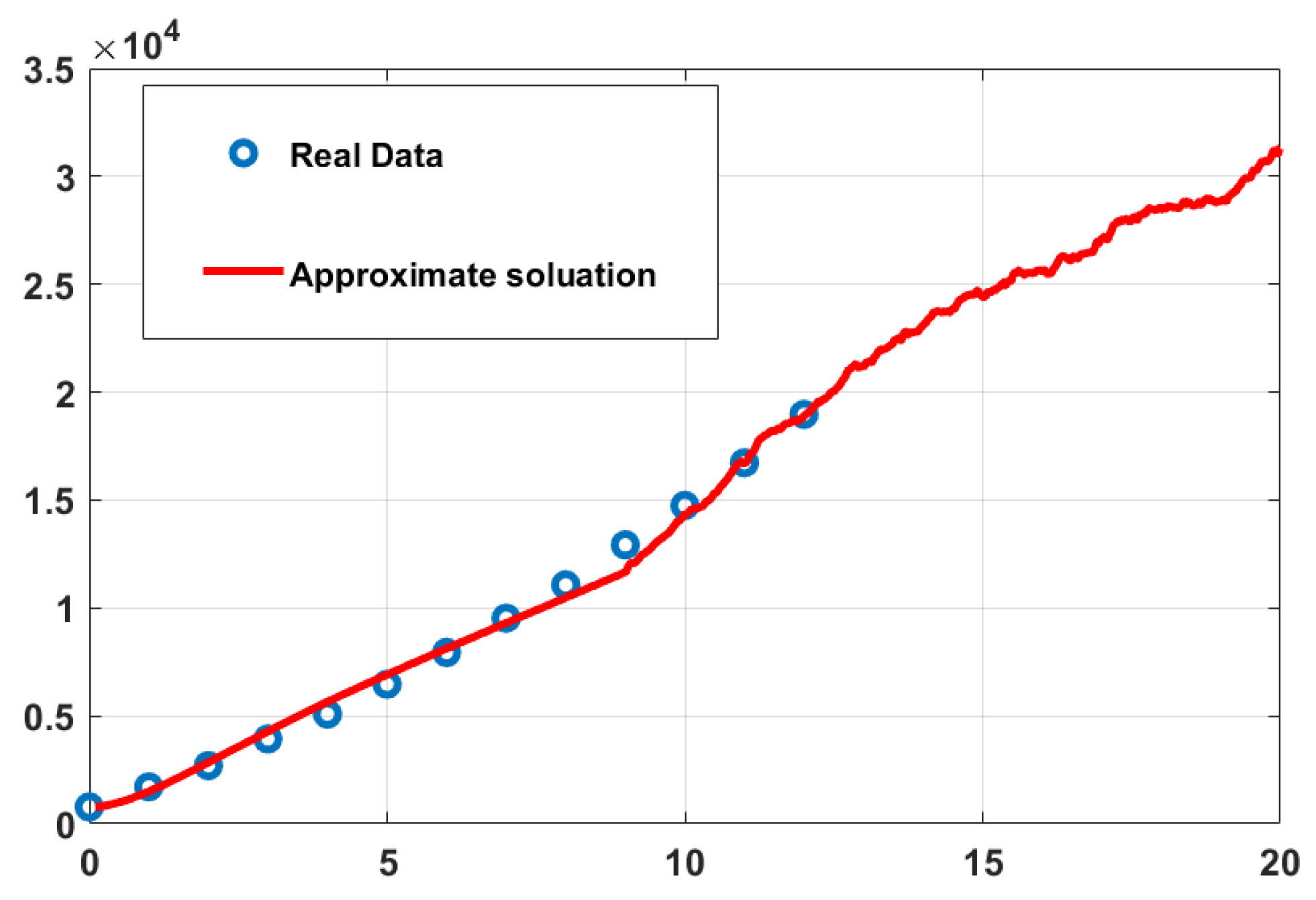
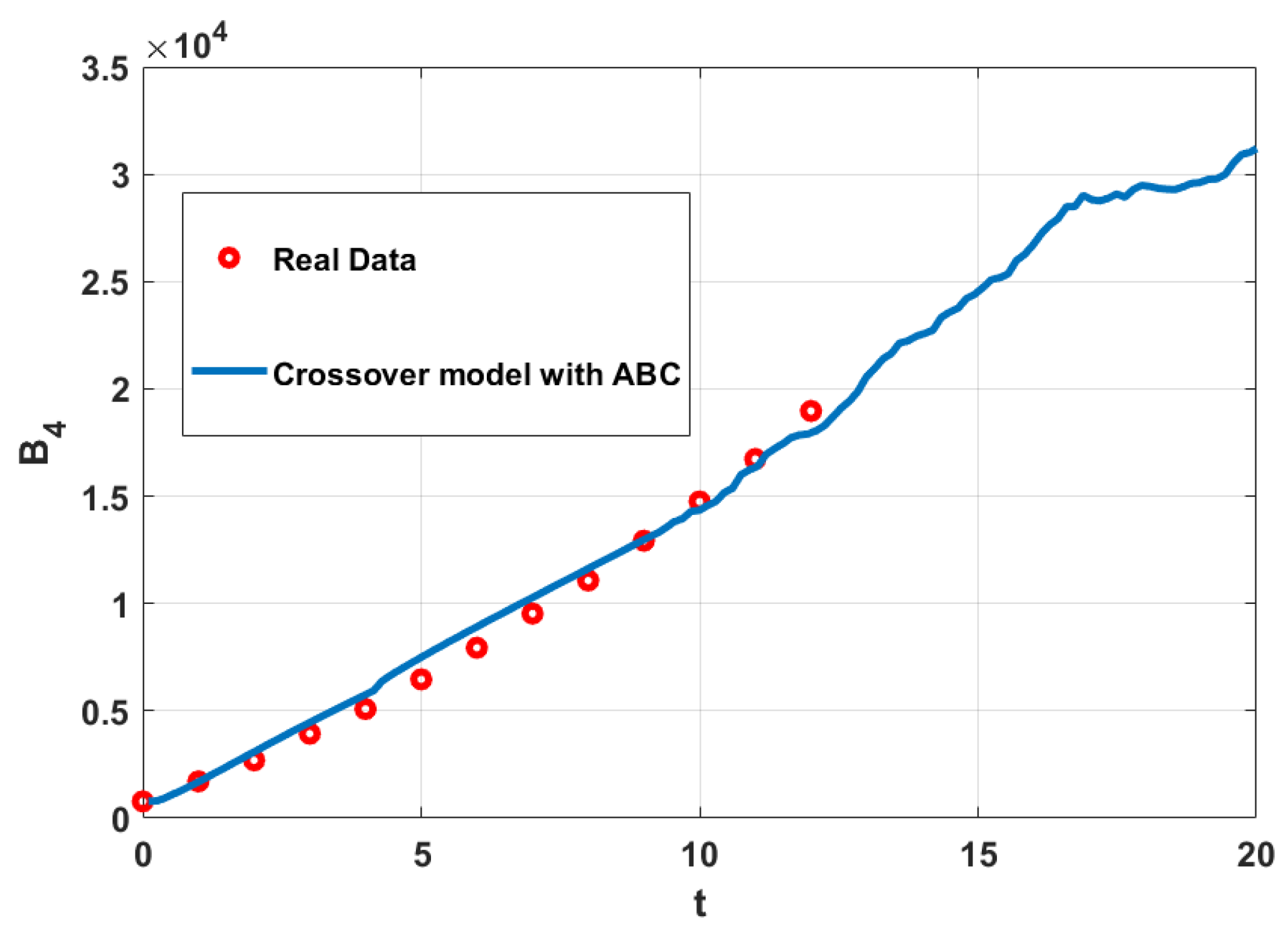
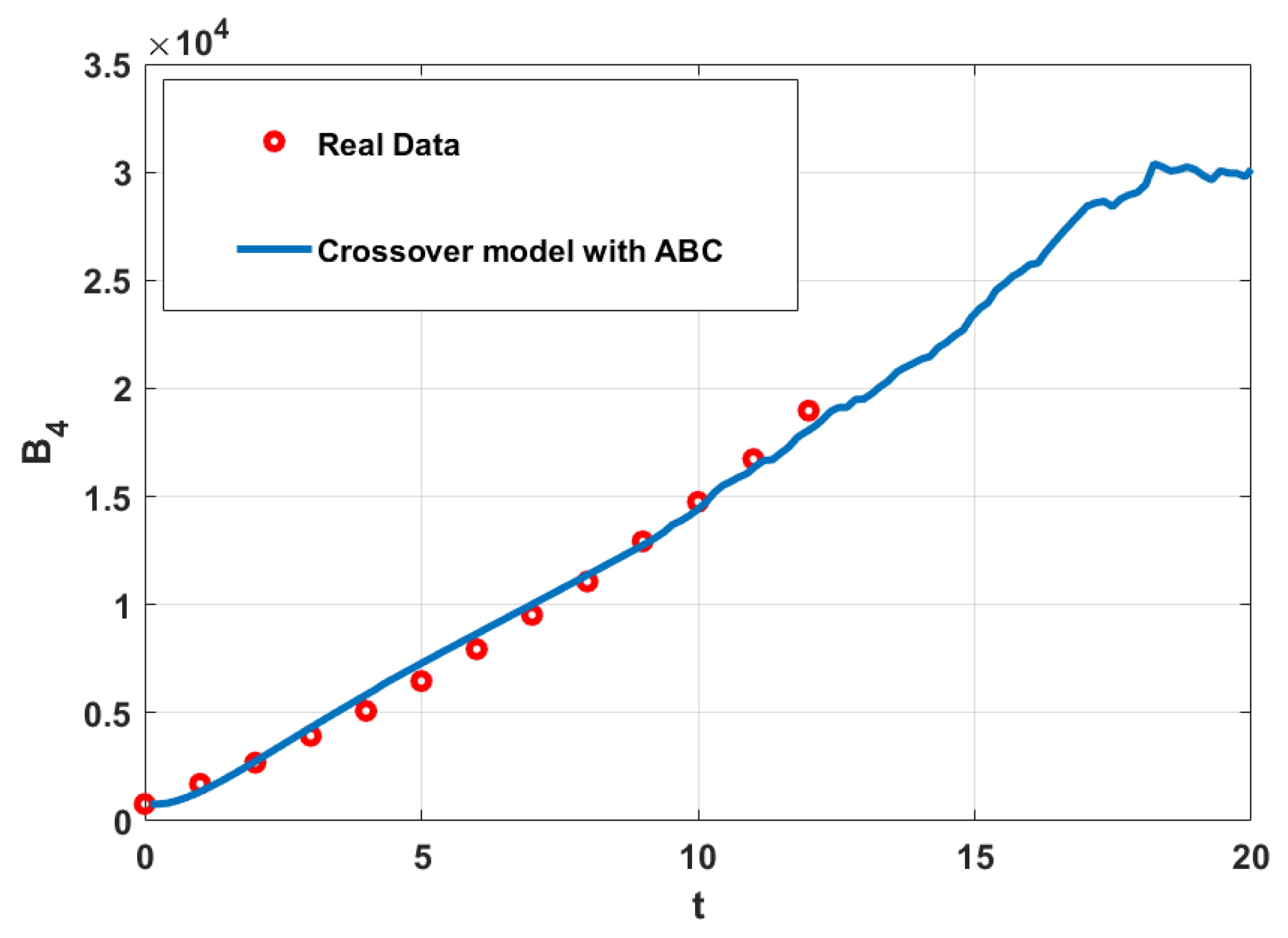
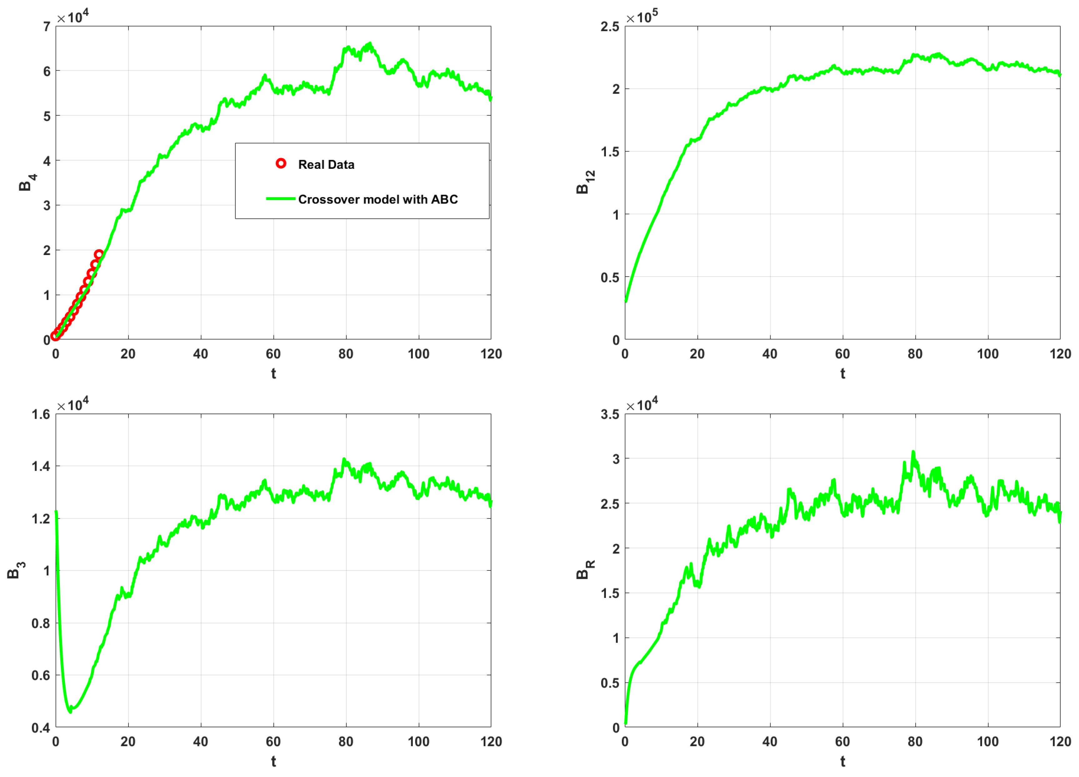
5. Numerical Simulations

We use the following parameters [4]: $\tau =0.01,$ $\Gamma =80,$ $\Omega =90,$ $\mu =0.01,$ $\varrho =0.03,$ $\upsilon =0.034,$ $\kappa =0.09,$ $\omega =0.1,$ $\Lambda =\mathrm{14,000},$ $\chi =0.0256,$ $\sigma =\left[0.350.5\right],$ $\xi =0.2,$ $\delta =0.0256,$ $\varsigma =0.0256,$ $\vartheta =0.03,$ $\varphi =0.3,$ ${\sigma }_1=0.1,{\sigma }_2=0.2,{\sigma }_3=0.02,{\sigma }_4=0.05,{\sigma }_5=0.02.$ Also, the initial conditions are given as follows: $B_{12}\left(t_0\right)=\mathrm{30,000},$ $B_3\left(t_0\right)=\mathrm{12,300},$ $B_4\left(t_0\right)=783,$ $B_R\left(t_0\right)=334,$ $B_E\left(t_0\right)=10,$ $\varpi \left(h\right)=1-e^{-h},$ $\Psi \left(t\right)={(\varsigma t+\lambda )}^{ϵ},$ $t_1=4,t_2=9,T_f=150.$ The crossover models are being validated against reported cases of stage four breast cancer among females in Saudi Arabia from 2004 to 2016 [4]. We compared the results of infected humans obtained from the proposed model (8)–(12) with real data in Figure 1, Figure 2, Figure 3, Figure 4, Figure 5, Figure 6, Figure 7 and Figure 8. In these Figures, we chose different values of $ϵ,\varsigma ,\lambda ,\mu ,\nu ,$ $\mu \left(t\right),\nu \left(t\right).$ We have excellent results compared with the models in [4]. The proposed model outperforms significantly. Also, we compared the results of stage four breast cancer patient incidences obtained from the proposed model (14)–(18) with real data in Figure 5 and Figure 6. Figure 7 shows the solution behavior for the considered model (14)–(18), when $H^{*}\left(t\right)=0.98-0.0007t$, and $\nu =0.96,$ $\mu =0.98,$ $\nu \left(t\right)=0.96-0.001{\left(cos(t/10)\right)}^2$ and $\mu \left(t\right)=0.96-0.001{\left(sin(t/10)\right)}^2.$ Also, the operators of $\Psi$-fractal fractional-order Caputo derivative and $\Psi$-fractal variable-order fractional Caputo derivative are more general than the operators of fractal fractional-order Caputo derivative and fractal variable-order fractional Caputo derivative, where when we put $\Psi \left(t\right)=t,$ we have the operators of fractal fractional-order Caputo derivative and fractal variable-order fractional Caputo derivative. Also, the proposed operators are more general than the fractal fractional-order Caputo–Katugampola derivative and fractal variable-order fractional Caputo–Katugampola derivative, when we put $\Psi \left(t\right)=t^{ϵ},$ we have the operators of the fractal fractional-order Caputo–Katugampola derivative and fractal variable-order fractional Caputo–Katugampola derivative. For our simulations in Figure 1, we use $\Psi \left(t\right)={(0.99t+0.97)}^{0.98};$ in Figure 2, we use $\Psi \left(t\right)=t^{ϵ};$ and in Figure 3, we use $\Psi \left(t\right)=t.$ Figure 8 shows the solution behavior for the considered model (8)–(12) with different values of $\mu ,\mu \left(t\right),\nu ,\nu \left(t\right)$, and $\Psi \left(t\right)={(0.99t+0.97)}^{0.98}.$ Figure 9 describes the effect of changing functions $\Psi \left(t\right)$ on the behavior of solutions and $\mu \left(t\right)=0.96-0.001sin{(t/10)}^2$ and $\nu =0.98,$ $\mu =0.98,$ $\nu \left(t\right)=0.98-0.001t$ and $\mu \left(t\right)=0.99-0.001t,$ ${\sigma }_1=0.01,$ ${\sigma }_2=0.02,$ ${\sigma }_3=0.02,$ ${\sigma }_4=0.05,$ ${\sigma }_5=0.02.$ From our results, using a simple nonstandard kernel function $\Psi \left(t\right),$ we outperformed previous classical and fractional models in [4].

6. Conclusions

This study focuses on examining two novel crossover models for breast cancer that incorporate $\Psi$-Caputo and Mittag-Leffler laws of fractal variable-order and fractal fractional-order derivatives. Three models of fractal variable-order, fractal fractional-order, and variable-order fractional stochastic derivatives are defined in three time sub-intervals. Two simple numerical methods were constructed to solve the suggested models based on $\Psi$-Caputo derivatives. These methods include $\Psi$-NSFDM to solve the deterministic models, and NMEMM is used to solve variable-order fractional stochastic differential equations generated by VFBM. We use real statistical data to validate our models. We have chosen this generalized Caputo operator for our work for several reasons, including its adaptability, capacity to capture complicated dynamics, and suitability for modeling fractional-order systems. Also, we use TAM to solve the second crossover model with a non-singular kernel. Overall, our $\Psi$-fractal variable-order fractional system can be reduced to a classical fractal fractional Caputo system using $\Psi \left(t\right)=t,\varsigma =1,ϵ=1,\lambda =0,$ and fractal variable-order fractional Caputo–Katugampola derivative when $\Psi \left(t\right)=t^{ϵ},\varsigma =1,\lambda =0.$ We demonstrated from comparing our results with real data that it is unnecessary to use non-trivial functions $\Psi \left(t\right)$ to advance the state of the art.

The current research investigation demonstrates that the $\Psi$-Caputo fractal fractional-order operator, with a simple nonstandard kernel function $\Psi \left(t\right)$ in this model, is one of the better options among the existing fractional-order operators. We outperform existing classical and fractal variable-order fractional models in the literature by using a simple nonstandard kernel function. In future work, we will extend this work to control the proposed model problem with time delay.

References

1. Fitzmaurice, C.; Dicker, D.; Pain, A.; Hamavid, H.; Moradi-Lakeh, M.; MacIntyre, M.F.; Allen, C.; Hansen, G.; Woodbrook, R.; Wolfe, C.; et al. The global burden of cancer 2013. JAMA Oncol. 2015, 1, 505–527. [Google Scholar] [CrossRef] [PubMed]
2. DeSantis, C.E.; Bray, F.; Ferlay, J.; Lortet-Tieulent, J.; Anderson, B.O.; Jemal, A. International variation in female breast cancer incidence and mortality rate international variation in female breast cancer rates. Cancer Epidemiol. Biomark. Prev. 2015, 24, 1495–1506. [Google Scholar] [CrossRef] [PubMed]
3. Tang, T.-Q.; Shah, Z.; Bonyah, E.; Jan, R.; Shutaywi, M.; Alreshidi, N. Modeling and analysis of breast cancer with adverse reactions of chemotherapy treatment through fractional derivative. Comput. Math. Methods Med. 2022, 2022, 5636844. [Google Scholar] [CrossRef]
4. Alzahrani, E.; El-Dessoky, M.; Khan, M.A. Mathematical model to understand cancer dynamics, prevention diagnosis, and therapy. Mathematics 2023, 11, 1975. [Google Scholar] [CrossRef]
5. Vasiliadis, I.; Kolovou, G.; Mikhailidis, D. Cardiotoxicity and cancer therapy. Angiology 2024, 65, 369–371. [Google Scholar] [CrossRef]
6. Dave, D.K.; Shah, T.P. Stability analysis and z-control of breast cancer dynamics. Adv. Appl. Math. Sci. 2021, 21, 343–363. [Google Scholar]
7. Solís-Pérez, J.E.; Gómez-Aguilar, J.F.; Atangana, A. A fractional mathematical model of breast cancer competition model. Chaos Solitons Fractals 2019, 127, 38–54. [Google Scholar] [CrossRef]
8. Chavada, A.; Pathak, N.; Raval, R. Fractional mathematical modeling of breast cancer stages with true data from Saudi Arabia. Results Control Optim. 2024, 15, 100431. [Google Scholar] [CrossRef]
9. Atangana, A.; Araz, S.İ. New concept in calculus: Piecewise differential and integral operators. Chaos Solitons & Fractals 2021, 145, 110638. [Google Scholar]
10. NSweilam, H.; AL-Mekhlafi, S.M.; Hassan, S.M.; Alsunaideh, N.R.; Radwan, A.E. A Novel Hybrid Crossover Dynamics of Monkeypox Disease Mathematical Model with Time Delay: Numerical Treatments. Fractal Fract. 2024, 8, 185. [Google Scholar] [CrossRef]
11. Alalhareth, F.K.; Al-Mekhlafi, S.M.; Boudaoui, A.; Laksaci, N.; Alharbi, M.H. Numerical treatment for a novel crossover mathematical model of the COVID-19 epidemic. AIMS Math. 2024, 9, 5376–5393. [Google Scholar] [CrossRef]
12. Awadalla, M.; Noupoue, Y.Y.Y.; Asbeh, K.A.; Ghiloufi, N. Modeling drug concentration level in blood using fractional differential equation based on Ψ-Caputo derivative. J. Math. 2022, 2022, 9006361. [Google Scholar] [CrossRef]
13. Wanassi, O.K.; Torres, D.F.M. Modeling blood alcohol concentration using fractional differential equations based on the Ψ-Caputo derivative. Math. Meth. Appl. Sci. 2024, 47, 7793–7803. [Google Scholar] [CrossRef]
14. Mohammadaliee, B.; Roomi, V.; Samei, M.E. SEIARS model for analyzing COVID-19 pandemic process via Ψ-Caputo fractional derivative and numerical simulation. Sci. Rep. 2024, 14, 723. [Google Scholar] [CrossRef]
15. Solis-Perez, J.E.; Gómez-Aguilar, J.F. Variable-order fractal-fractional time delay equations with power, exponential and Mittag-Lefer laws and their numerical solutions. Eng. Comput. 2022, 38, 555–577. [Google Scholar] [CrossRef]
16. Gómez-Aguilar, J.F.; Rosales-García, J.J.; Bernal-Alvarado, J.J.; Córdova-Fraga, T.; Guz-mán-Cabrera, R. Fractional mechanical oscillators. Rev. Mex. Fis. 2012, 58, 348–352. [Google Scholar]
17. Gómez-Aguilar, J.F.; Atangana, A. New insight in fractional differentiation: Power, exponential decay and Mittag-Leffler laws and applications. Eur. Phys. J. Plus 2017, 132. [Google Scholar] [CrossRef]
18. Haq, I.; Ali, N.; Ahmad, H.; Sabra, R.; Albalwi, M.D.; Ahmad, I. Mathematical analysis of a coronavirus model with Caputo, Caputo-Fabrizio–Caputo fractional and Atangana–Baleanu–Caputo differ-ential operators. Int. J. Biomath. 2023, 23, 2350085. [Google Scholar] [CrossRef]
19. Ul Haq, I.; Ali, N.; Bariq, A.; Akgül, A.; Baleanu, D.; Bayram, M. Mathematical modeling of COVID-19 outbreak using Caputo fractional derivative: Stability analysis. Appl. Math. Sci. Eng. 2024, 32, 2326982. [Google Scholar] [CrossRef]
20. Owolabi, K.M.; Atangana, A. On the formulation of Adams-Bashforth scheme with Atan-gana-Baleanu-Caputo fractional derivative to model chaotic problems. Chaos 2019, 29, 023111. [Google Scholar] [CrossRef]
21. Toufik, M.; Atangana, A. New numerical approximation of fractional derivative with non-local and non-singular kernel: Application to chaotic models. Eur. Phys. J. Plus 2017, 132, 1–16. [Google Scholar] [CrossRef]
22. Kumar, A.; Shaw, P.K.; Kumar, S. Numerical investigation of pine wilt disease using frac-tal-fractional operator. Indian J. Phys. 2024. [Google Scholar] [CrossRef]
23. Kumar, S.; Chauhan, R.P.; Momani, S.; Hadid, S. Numerical investigations on COVID-19 model through singular and non-singular fractional operators. Numer. Methods Part. Differ. Equ. 2024, 40, e22707. [Google Scholar] [CrossRef]
24. Samko, S.G.; Kilbas, A.A.; Marichev, O.I. Fractional Integrals and Derivatives; Gordon and Breach Science Publishers: Yverdon, Switzerland, 1993. [Google Scholar]
25. Kilbas, A.A.; Srivastava, H.M.; Trujillo, J.J. Theory and Applications of Fractional Differential Equations; North-Holland Mathematics Studies; Elsevier Science B.V.: Amsterdam, The Netherlands, 2006. [Google Scholar]
26. Almeida, R.; Malinowska, A.B.; Monteiro, M.T.T. Fractional differential equations with a Caputo derivative with respect to a kernel function and their applications. Math. Methods Appl. Sci. 2018, 41, 336–352. [Google Scholar] [CrossRef]
27. Atangana, A. Fractal-fractional differentiation and integration: Connecting fractal calculus and fractional calculus to predict complex system. Chaos Soliton Fract. 2017, 102, 396–406. [Google Scholar] [CrossRef]
28. Mickens, R.E. Nonstandard Finite Difference Models of Differential Equations; World Scientific: Singapore, 2005. [Google Scholar]
29. Atangana, A.; Qureshi, S. Modeling attractors of chaotic dynamical systems with frac-tal-fractional operators. Chaos Solitons Fractals 2019, 123, 320–337. [Google Scholar] [CrossRef]
30. Sweilam, N.H.; AL-Mekhlafi, S.M.; Mohamed, D.G. Novel chaotic systems with fractional differential operators: Numerical approaches. Chaos Solitons Fractals 2021, 142, 110475. [Google Scholar] [CrossRef]
31. Hu, Y.; Liu, Y.; Nualart, D. Modified Euler approximation scheme for stochastic differential equations driven by fractional Brownian motions. arXiv 2013, arXiv:1306.1458. [Google Scholar]
32. Atangana, A.; Araz, S. New Numerical Scheme with Newton Polynomial Theory, Methods, and Applications; Academic Press: Cambridge, MA, USA, 2021. [Google Scholar]
Figure 1. Breast cancer data from Saudi Arabia compared with the obtained results for (8)–(12) when μ ( t ) = 0.99 0.001 t , ν ( t ) = 0.98 0.001 t ,   ϵ = 0.98 ,   λ = 0.97 ,   ς = 0.99 ,   H * ( t ) = 1 0.001 t , μ = 0.99 ,   ν = 0.99 .
Symmetry 16 01172 g001
Figure 2. Breast cancer data from Saudi Arabia compared with the obtained results for (8)–(12) when μ ( t ) = 0.99 0.001 t , ν ( t ) = 0.98 0.001 t ,   ϵ = 0.98 , λ = 0 ,   ς = 1 ,   H * ( t ) = 1 0.001 t ,   μ = 0.99 , ν = 0.99 .
Symmetry 16 01172 g002
Figure 3. Breast cancer data from Saudi Arabia compared with the obtained results for (8)–(12) when μ ( t ) = 0.99 0.001 t , ν ( t ) = 0.98 0.001 t ,   ϵ = 1 ,   λ = 0 ,   ς = 1 ,   H * ( t ) = 1 0.001 t ,   μ = 0.99 ,   ν = 0.99 .
Symmetry 16 01172 g003
Figure 4. Breast cancer data from Saudi Arabia compared with the obtained results for (8)–(12) when μ ( t ) = 0.99 0.001 t , ν ( t ) = 0.98 0.001 t ,   ϵ = 0.98 ,   λ = 0 ,   ς = 1 ,   H * ( t ) = 1 0.001 t and different values of ν and μ .
Symmetry 16 01172 g004
Figure 5. Breast cancer data from Saudi Arabia compared with the obtained results for (14)–(18) when μ ( t ) = 0.99 0.001 t , ν ( t ) = 0.98 0.001 t ,   H * ( t ) = 1 0.001 t and ν = 0.98 and μ = 0.90 .
Symmetry 16 01172 g005
Figure 6. Breast cancer data from Saudi Arabia compared with the obtained results for (14)–(18) when μ ( t ) = 0.99 0.001 t , ν ( t ) = 0.99 0.001 ( c o s ( t / 10 ) ) 2 ,   H * ( t ) = 1 0.001 t and ν = 0.98 and μ = 1 .
Symmetry 16 01172 g006
Figure 7. Simulation for (14)–(18) with H * ( t ) = 0.98 0.0007 t , and ν = 0.96 , μ = 0.98 , ν ( t ) = 0.96 0.001 ( c o s ( t / 10 ) ) 2 and μ ( t ) = 0.96 0.001 ( s i n ( t / 10 ) ) 2 .
Symmetry 16 01172 g007
Figure 8. Simulation for (8)–(12) with ϵ = 0.98 ,   λ = 0.97 ,   ς = 0.99 ,   H * ( t ) = 1 0.001 t , and different values of ν ,   μ ,   ν ( t ) and μ ( t ) .
Symmetry 16 01172 g008
Figure 9. Simulation for (8)–(12) with different Ψ ( t ) ,   H * ( t ) = 1 0.001 t , and ν = 0.98 ,   μ = 0.98 ,   ν ( t ) = 0.98 0.001 t and μ ( t ) = 0.99 0.001 t .
Symmetry 16 01172 g009aSymmetry 16 01172 g009b