Abstract
The measurement of mixing time in a water model of soft-stirring steelmaking ladles is practically facing a problem of bad repeatability. This uncertainty severely affects both the understandings of transport phenomenon in ladles and the measurement accuracy. Scaled down by a ratio of 1:4, a water model based on an industrial 260-ton ladle is used. This paper studies the transport process paths and mixing time of salt solution tracers in the water model of eccentric gas-stirred ladles with a low gas flow rate. After a large number of repeated experiments, the different transport paths of the tracer and the error of the mixing time in each transport path are discussed and compared with the numerical simulation results. The results of a large number of repeated experiments on the water model show that there are five transport paths for the tracer in the ladle. The tracer of the first path is mainly transported by the left-side main circulation flow, which is identical to the numerical simulation results. The tracer of the second and third paths are also mainly transported by the left-side circulation flow, but bifurcations occur when the tracer in the middle area is transported downward. In the third path, the portion and intensity of the tracer transferring to the right side from the central region is higher than in the second path. The fourth path is that the tracer is transported downward from the left, middle, and right sides with a similar intensity at the same time. While the tracer in the fifth path is mainly transported on the right side, and the tracer forms a clockwise circulation flow on the right side. The mixing times from the first transport path to the fifth transport path are 158.3 s, 149.7 s, 171.7 s, 134 s and 95.7 s, respectively, among which the third transport path and the fifth transport path are the maximum and minimum values among all transport paths. The error between the mixing time and the averaged mixing time at each monitoring point in the five transport paths of the tracer is between −34.7% and 40.9%. Furthermore, the error of the averaged mixing time of each path and the path-based average value is between 5.5% and 32.6%.
1. Introduction
The steelmaking ladle with gas stirring has been widely used in steel industries [1,2,3], where they promote alloy and steel scrap melting [4,5,6,7,8,9], accelerate metallurgical reactions at the steel-slag interface [10,11,12,13], hence facilitating the homogenization of chemical composition and temperature of molten steel [3,14], eliminate non-metallic inclusions in the steel [15,16,17,18,19,20], and effectively enhance steel product quality [21,22]. Gas stirring is the key factor for mixing chemical composition and temperature. Conejo [23,24] pointed out that the mixing of liquid steel in ladles and the mass transfer in slags for chemical reactions cannot be achieved simultaneously.
Regarding gas injection location, Conejo [24] also pointed out that a central gas injection promotes mass transfer and refining rates, while an off-central asymmetrical gas injection promotes the mixing efficiency of liquid steel. Center gas stirring can cause many problems, such as a non-uniform composition after alloy additions and a weak stirring efficiency [4,5,25,26,27,28,29,30]. Asymmetrical gas stirring is widely used in small-tonnage ladles and will be the focus in this study.
Over the past several decades, as summarized in the reviews [31,32,33], physical models, i.e., water models [34,35,36,37,38,39,40,41,42,43,44,45,46,47,48,49,50,51,52,53,54] and numerical models [55,56,57,58,59,60,61,62,63,64,65,66,67,68,69,70], have been widely established to study the transport phenomenon in gas-stirred ladles. Specifically, the effects of gas flow rate, as well as the location, number, size, and separation angle of stirring plugs on fluid flow and the mixing process in gas-stirred ladles, were investigated using water models [71,72,73,74,75,76,77,78,79,80,81,82,83].
In water model experiments, the ladle flow field is usually studied by the colorimetric method or by analysis of photos of ink. In the past few decades, researchers have used tracer substances such as colored dyes [16,39,84,85,86,87,88], food coloring [89], and KMnO4 solution [47,90,91] to study flow field behavior in the ladle. However, this method cannot quantitatively study mixing behavior in the ladle. The mixing time in water models is used to evaluate the mixing performance and operational efficiency of a metallurgical ladle [71,72,73,74,75,76,77,78,79,80,81,82,83,92]. Taylor et al. [93] assessed a method for measuring mixing time using various types of tracers. In the experiment, conductivity monitoring points were usually placed at special locations in the ladle to monitor changes in the tracer concentration of the solution [92], and then the mixing time of the ladle was obtained. In previous studies, scholars studied the effects of the monitoring point location and tracer addition location [42,88,94,95,96,97], porous plug layout [10,45,74,77,78,79,80,81,85,87,98], stirring method [86,90,99], water model ratio [100] and top slag layer [45,72,82] on the mixing time of the ladle. Salt solution tracers such as saturated KCl solution [101,102] and saturated NaCl solution [85,103,104,105] have been widely used, but the density of these tracers are 16.6% and 19.9% higher than water at room temperature, respectively. This density difference affects the fluid flow and measured mixing time.
Chen et al. [106,107,108] and Ding et al. [109,110] conducted in-depth studies on the impact of salt tracers on fluid dynamics in continuous flow reactors. It was found that during the injection of salt solution tracers, the tracer flowed downward and accumulated at the bottom in tundishes. Similar research focused on the effects of fluid flow in batch reactors, such as vacuum refining furnaces [111,112,113] and bottom-blown gas-stirred ladles [114,115,116,117]. Like earlier studies, Krishna-Murthy et al. [40] concluded that mixing time is not influenced by variations in the amount of tracer used. Until recently, Chen et al. [114] discovered that increasing the tracer volume can shorten the measured mixing time. Gómez et al. [115] observed that tracer concentration influences the mixing time, but the effect is significant only at low gas flow rates. Zhang et al. [116] used numerical simulations to demonstrate that the mixing process of a saturated KCl solution is faster than that of a pure water tracer, and the salt solution tracer accumulates at the bottom of the ladle. The corresponding industrial gas flow rate can be calculated by the experimental flow rate and the scale factor. The equivalent industrial gas flow rates were 730 NL·min−1 in the studies conducted by Chen et al. [114] and Zhang et al. [116]. However, in the studies conducted by Gómez et al. [115], these gas flow rates were 610 NL·min−1, 1435 NL·min−1, and 2153 NL·min−1. These gas flow rates are very large for industrial practical operations. Thus, the above mentioned studies were based on ladles with high gas flow rates.
Recently, Li et al. [117] studied the effect of tracer dosage on mixing time at moderate gas flow rates. The study found that the concentration curve of the tracer at the monitoring point located in the bottom-right area of the ladle had two trends. The first trend showed the injected salt solution tracer asymmetrically transported by the main circulation toward the left side wall of the ladle. In the second trend, the tracer was carried by both the main circulation to the left side wall and by a downward flow toward the gas column. Finally, Li et al. [117] also proposed further studies on the low gas flow rate conditions. However, in the study, the equivalent industrial gas flow rate was 700 NL·min−1, which is relatively larger than the common practice of soft stirring, for example 200 to 500 NL·min−1. In practical operations, the gas stirring flow rate varies during the refining process, i.e., there is a higher gas flow rate during the start stage for a better performance melting of refining agents and alloys, and there is a lower gas flow rate at the end of the operation for inclusion removal and less heat loss. Based on this information, this paper will study the transport of tracers in low gas flow rate conditions.
From the authors’ observations as well as communications with many researchers, the measurement of mixing time in a water model of soft stirring steelmaking ladles is practically facing a problem of bad repeatability. This uncertainty severely affects both the understandings of transport phenomenon in ladles and measurement accuracy. This study investigates the transport pathways and mixing time of a salt solution tracer in a scaled-down water model of a 260-ton industrial ladle (1:4 ratio), focusing on an asymmetrical gas-stirred ladle with a low gas flow rate.
2. Materials and Methods
2.1. Physical Model Experiment
2.1.1. Water Model Size
Based on the principle of geometric similarity, this study employs a 260-ton ladle as a prototype. A ladle experimental device is scaled down to a ratio of 1:4. Table 1 shows the model parameters of the ladle experimental device. The experimental device is made of plexiglass and is equipped with a fixed frame, an air compressor, a flow meter, a conductivity meter, computers, and other equipment. In the physical simulation experiment, compressed air is used to simulate argon, and water is used to simulate molten steel. Using a volume of 100 mL of saturated KCl solution and 7 mL of ink as a mixed tracer, the transport process of the tracer within the ladle can be visualized.

Table 1.
Ladle model parameters.
In order to determine the flow rate of gas blown during the experiment, it is necessary to consider the dynamic similarity between the prototype ladle and the model. The method commonly used by researchers is to use the modified Froude number similarity to confirm that the dimensionless numbers for the two systems are the same. This paper uses the dimensionless variable G obtained by Krishnaposharody and Irons [118] to satisfy the dynamic similarity:
Dimensionless number G
where U refers to the gas characteristic velocity in m·s−1, and U is calculated as U = Q/A, where Q refers to the gas flow rate in m3·h−1, and A refers to the plug area in m2. and are the density of gas and liquid, kg·m−3; g refers to the acceleration of gravity, m·s−2; H refers to the level of liquid height in the ladle, m; and d refers to the diameter of the injection nozzle, in meters (m).
Therefore, the conversion relationship between the model (m) and the prototype (p) should satisfy the following [119]:
where and refer to the density of air and water at room temperature, kg·m−3; and refer to the densities of argon gas and liquid steel at steelmaking temperature, kg·m−3; refers to the flow rate of argon at steelmaking temperature, m3·h−1; refers to the experimental air flow rate at room temperature, m3·h−1; and d refers to the diameter of the plug, m.
In the actual steelmaking process, as the gas enters the ladle, its flow rate will vary due to changes in temperature and pressure. Therefore, it is necessary to correct for temperature and pressure variations:
where: and represent the temperatures of molten steel and room temperature, K; and are the standard atmospheric pressure and the gas pressure at ladle outlet, Pa., and ; and refers to the argon flow rate under standard conditions, m3·h−1 [117].
In summary, when the water model ratio is 1:4 and the original gas flow rate is 400 L/min, after calculation, the gas flow rate used in the experiment is 2.3 L/min.
2.1.2. Experimental Program
Figure 1 shows the schematic diagram of the ladle water model experiment. At the start of the experiment, the liquid level in the ladle water model was set to 821 mm. Compressed air, with a flow rate of 2.3 L/min, was introduced through the porous plug situated 0.2 radii from the center at the bottom of the ladle. Two conductivity monitoring points were installed on the side close to the porous plug in the ladle water model, named monitoring point 1 and monitoring point 2, and a conductivity monitoring point was installed on the side away from the porous plug, named monitoring point 3.
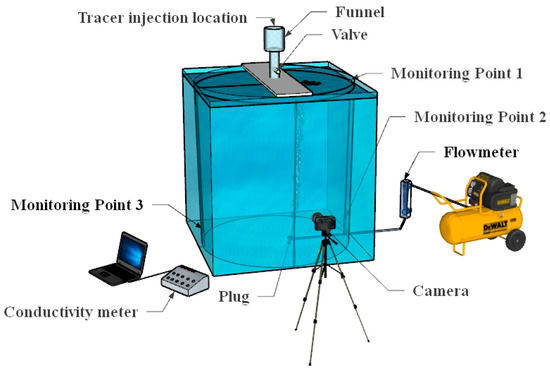
Figure 1.
Experimental diagram of ladle.
After the ladle flow field became stable, the tracer solution was added to the funnel, which is fixed at the position just above the ladle. When the experiment starts, the valve is manually opened for injection of the tracers in the funnel. Simultaneously, the photos of the black-ink-mixed tracer were recorded by a high-resolution camera. Later, the evolution of the black-ink photos were used for visualization. Meanwhile, the conductivity data were monitored and measured immediately after injection of the mixed tracer. Based on the stimulus–response method, the time when the conductivity changes does not exceed ±5% of the stable value, and it was determined as the mixing time.
In this study, we started working only on the conductivity and mixing time measurements, but after a while, we found a bad repeatability for the curves at the bottom monitoring points. Then, we started the black ink and KCl solution mixed tracer experiments by both recording the photos of the tracer and measuring the conductivity data. We repeated the experiment approximately 30 times and found out there were mainly five transport paths of the tracer, which will be presented in the later sections.
2.2. Numerical Simulation
2.2.1. Model Assumptions
The Euler–Euler method was employed to perform numerical simulations of gas–liquid multiphase flow within a ladle water model, underpinned by four key assumptions: (1) the gas and liquid phases are characterized as incompressible Newtonian fluids, devoid of chemical reactions during the gas’s upward trajectory; (2) the solid walls are defined as non-slip surfaces, with wall functions applied near the walls; (3) the simulations disregard the effects of temperature; and (4) the bubble dimensions are presumed to be invariant during the simulation, with no coalescence or fragmentation events taking place during transport.
2.2.2. Euler–Euler Model
The Euler–Euler model treats each phase encountered in the simulation as a distinct continuous medium, with each phase possessing its conservation equations. To accurately simulate two-phase flow dynamics, the continuity and momentum conservation equations for each phase must be clearly defined. In these momentum equations, the forces exerted by the gas and liquid phases on each other are recognized as sources of momentum exchange.
Continuity equation:
In the present study, the gas phase is designated as the dispersed phase, with the liquid phase serving as the continuous phase. Temperature effects are disregarded, and the flow dynamics of the water model are simulated at room temperatures. Here are the continuity equations for the two phases.
In the equations, refers to the volume fraction of phase k; denotes the density of phase k; and signifies the velocity of phase k.
Momentum equation
In these equations, denotes the interfacial momentum transfer between the gaseous and liquid phases, which is equivalent to the interfacial force exerted on phase .
Interfacial forces:
During the computational process, the interfacial forces are primarily composed of lift, drag, turbulent dissipation forces, and virtual mass forces.
In the equations, , , , representing lift, drag, virtual mass forces, and forces of turbulent dissipation, representing the momentum transfer phase from the gas phase (liquid phase) to the liquid phase (gas phase).
Drag Force:
The drag force represents the opposing resistance applied to the bubbles by the gas and liquid phases alike, which acts in the direction opposite to the bubble’s motion.
In these equations, represents the drag coefficient. This numerical simulation is conducted under room temperature and standard pressure conditions, specifically targeting the liquid phase dynamics within a steel ladle water model. The drag coefficient is fitted using a curve fitting method based on a proposal by Wang [120].
Lift Force:
Lift force, the aerodynamic force responsible for the upward motion of an object, necessitates a consideration of multiple fluid properties, including viscosity and compressibility. For the current experimental investigation, we utilized the Kutta–Joukowski theorem, which is formulated as:
The equations employed in this research involve the calculation of the symmetric interaction area density, which is derived from the lift coefficient and the lift correction factor , as follows:
According to Lou and Zhu [121], a comparison of the lift coefficient constants in the Euler–Euler model for gas–liquid two-phase flow reveals that when the lift coefficient is positive, the gas column in the steel ladle water model exhibits a converging behavior, whereas when the lift coefficient is negative, the gas column in the steel ladle water model tends to diverge.
Virtual Mass Force:
The fluid within the ladle water model influences the acceleration of the streaming gas bubbles. The inviscid flow theory refers to this effect as “virtual mass,” which is equivalent to a constant multiplied by the gas flow rate displaced by the bubble. The expression is as follows:
The equations represent the virtual mass coefficient. and represent the accelerations of the gas phase and liquid phase, respectively [112].
Turbulent Dissipation Force:
Modeled as the turbulent dissipation force, it results from the interaction between the dispersed phase and the surrounding vortex flow.
The equations denote the relative velocity, which is defined by the volume fraction-weighted average of the velocities of the respective phases. represents the tensor diffusion coefficient.
2.2.3. Turbulence Model
This study uses the Realizable k-ε two-layer turbulence model for numerical simulations, which calculates the turbulent kinetic energy k and the turbulent dissipation rate ε. Below is its formula:
kinetic energy k
turbulent dissipation rate ε
where and are production terms that depend on the k-ε model; , , , and are constant, and their values are 1, 1.2, 1.44, and 1.9, respectively. represents the turbulent kinetic energy generated by the mean velocity gradient; denotes the magnitude of the mean strain rate tensor; and stands for the velocity gradient.
In the vicinity of the wall, the turbulent dissipation rate ε in the two-layer model is a function of the distance from the wall surface, which can be expressed as:
The equations represent the characteristic length scale. Within the context of the Eulerian–Eulerian model, the shear-driven approach proposed by Wolfshtein [122] utilized:
In the formula,
where refers to the distance to the wall and refers to the wall-distance Reynolds number.
2.2.4. Tracer Transport Model
In the batch reactors, to realistically simulate the tracer injection process in water models, a tracer injection inlet was set at the center of ladle surface. This method is similar to our previous work [111,112,113,116]. The tracer transport model is a total mass fraction based model, which is similar to the passive scalar model. However, the density of the mixed fluid was coupled with the density of KCl solution. The model is described as follows.
where is the mass fraction of the overall KCl solution in the computational domain. When tracers were introduced through the top inlet of the water model = 1, that meant the cell was filled with tracer [123]. When tracer addition stopped, = 0, that meant the cell was filled with water. Note that this equation is not the chemical concentration of KCl solute but rather the mass fraction of KCl solution in the cell and will be shortened as “mass fraction of KCl solution” in later sections. The effective diffusion coefficient is the sum of the molecular diffusion coefficient and turbulent diffusion coefficient, as follows.
where is the molecular diffusion coefficient of liquid phase, and is the turbulent diffusion coefficient,
In all the continuity, momentum, and turbulence equations, the density of the mixing fluid is calculated as follows.
where and represent the density of water and tracer, respectively.
2.2.5. Boundary Conditions
- In this simulation, the walls (for example, the bottom and side walls) of the ladle were set to a wall, i.e., non-slip boundary condition.
- The ladle’s surface was treated with a phase permeability condition that lets gas bubbles escape while stopping the liquid phase from penetrating.
- The inlet of the porous plug was set to a velocity inlet, and the velocity was calculated according to the gas flow rate.
- For the tracer inlet, during the tracer injection time interval, the tracer inlet was set to a velocity inlet and the mass fraction of the tracer was set to 1. After the injection of the tracer was completed, the tracer inlet was set to the phase permeable wall condition, which is identical to the free surface. Additionally, a mass fraction of 0 was assigned to the tracer inlet.
- For the tracer concentration on all the walls and surface, the zero flux condition was utilized.
- The turbulent kinetic energy and turbulent dissipation rate of the gas phase at the gas inlet were calculated using the method proposed by Ilegbusi et al. [124].
In this context, denotes the radius of the orifice, measured in meters [113].
2.3. Solution Process
In this simulation, the ladle model was meshed using the directional mesh method, which generates a tetrahedral mesh on the model surface. The front view and bottom view of the mesh established in the experiment are shown in Figure 2. A mesh independent test was performed and will be presented in the next section.
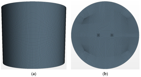
Figure 2.
Mesh generation. (a) front view; (b) bottom view.
The numerical simulation calculation uses STAR-CCM+ software 13.04 [125] to simulate the flow field under a single porous plug blowing in the ladle and the tracer mixing process. The geometric model established based on the ladle water model has the same geometric dimensions, blowing position, blowing flow rate, tracer injection position, and monitoring point position as the water model.
3. Results
3.1. Numerical Simulation Result
3.1.1. Mesh Independence
The mesh independence was verified by monitoring the changes in the liquid phase and gas phase velocity at different heights from the blowing position at the bottom of the ladle to the top of the ladle. The results and monitoring line are shown in Figure 3. Under three different numbers of meshes (288,960; 367,425; and 490,048), the liquid phase velocity at different height monitoring points changes slightly, while the gas phase velocity changes insignificantly and can be acceptable. Therefore, the effect of the number of meshes on the simulation results can be ignored. The mesh with 288,960 meshes is finally used in this simulation.
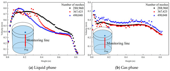
Figure 3.
Liquid phase and gas phase velocity changes at monitoring points at different heights under three kinds of mesh quantities. (The red line in the picture is the monitoring line, and the blue dot above and the red monitoring line are a whole).
3.1.2. Numerical Simulation Results of Tracer Transport Process
Figure 4 shows the numerical simulation results of the tracer transport process in the longitudinal section of the ladle. The gas inlet is eccentrically placed at the bottom of the right part of this cross section. As can be seen from Figure 4, the transport process of the tracer in the longitudinal section can be divided into five steps:
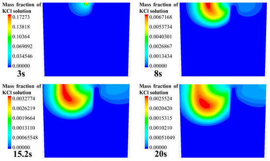
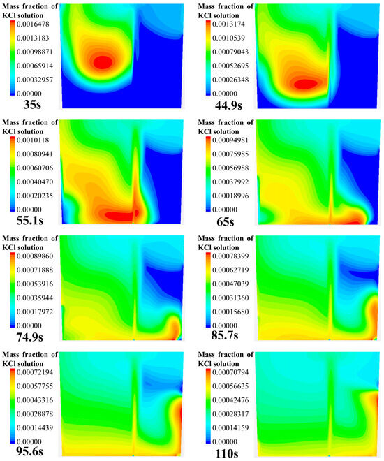
Figure 4.
Tracer transport process in the longitudinal section of the ladle.
- (1)
- When the tracer is added from the center directly above the ladle, the tracer first transports on the free surface of the ladle toward the left and right sides. At around 8 s, the tracer on the left begins to transport downward. (Note that the left means the direction away from the gas inlet, the right means the direction that is opposite, and this applies in all the later sections).
- (2)
- At 15 to 20 s, the tracer on the left side of the gas column has moved to the left wall of the ladle, and the front of the tracer is located at half the height of the liquid level. At the same time, on the right side of the gas column, the tracer has just dispersed to the vicinity of the right wall.
- (3)
- At 35 to 45 s, the tracer on the left side continues to move toward the bottom of the ladle along the left wall. At 45 s, the diffusion front of tracer is located at the bottom of the left side, and the tracer continues to transport along the bottom toward the right side of the ladle. At this time, the tracer on the right side still stays in the upper right area of the ladle.
- (4)
- At 55~65 s, the tracer on the left side of the gas column moves toward the right wall along the bottom of the ladle. When the tracer passes the gas column, a portion of the tracer is brought to the free surface of the ladle by the gas column, and the other portion of the tracer continues to move toward the right wall along the bottom of the ladle.
- (5)
- At 75~110 s, the tracer flows from the bottom of the left side of the ladle, reaching the right wall, and it gradually transports upwards to the upper right side of the ladle due to the influence of the main circulation. At this time, the concentration of the tracer in the ladle is relatively low. The tracer near the upper right wall of the ladle is transported downward to the ladle. The tracers in the whole ladle gradually reaches the mixing.
For a better illustration of the mixing mechanism, the turbulent viscosity of water is shown in Figure 5. For this Euler–Euler model, the turbulent viscosity of the gas phase is not presented due to the fact that the KCl solution dissolved in the water fluid phase. The turbulent viscosity, which indicates turbulent diffusion, shows a higher value at the top surface and near the top area of the gas column. In contrast, for example, at the bottom area, the diffusion of the KCl solution by turbulent diffusion is weaker. The molecular diffusion may play an important role in the mixing process.
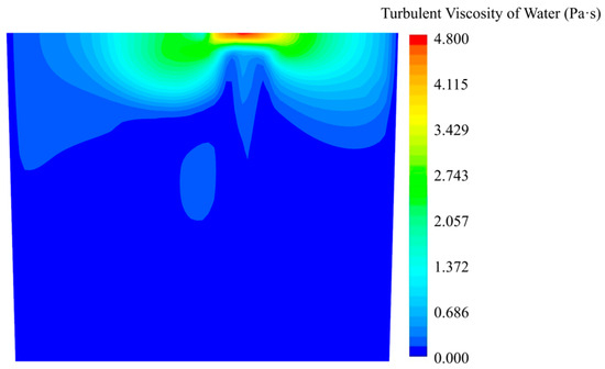
Figure 5.
Turbulent viscosity of water in simulation.
Figure 6 shows the tracer transport process and the three-dimensional streamlines in the ladle. The simulation case is the same as that shown in Figure 4. It can be seen from the transport process of the tracer in the streamline that the overall transport process of the tracer in the ladle is consistent with Figure 4. As shown in Figure 6, the flow in the ladle consists of the left-side anticlockwise main circulation and a weak clockwise circulation in the upper right area. The tracer is transported asymmetrically, i.e., it flows along the surface to the left side and moves downward along the left side of the ladle following the main circulation flow. After the tracer moves to the left bottom, it transports along the bottom toward the right side of the ladle. Due to the influence of the main circulation, the tracer gradually transports upward along the right side wall. However, the tracer on the upper right side does not spread to other regions, and the tracer is mixed in the weak circulation in the end.
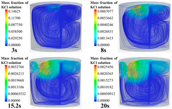
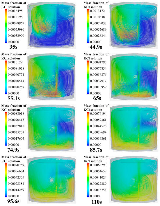
Figure 6.
Tracer transport process in ladle.
3.2. Tracer Transport Path and Analysis
The transport process of salt solution tracers in the water model of ladles is still unknown, and the addition of salt solution tracers will affect the flow field structure, resulting in certain changes in the tracer transport path. In this section, the photos of black ink tracers are manually marked by red lines to determine the boundaries of the black parts and non-diffused parts. Through an analysis of the evolution of this boundary at different times, the transport or dispersion of tracers can be visualized. For tracer concentration curves, there are two different types: namely, the sinusoidal and parabolic types [126,127], which represent two types of tracer transport paths. These tracer transport types will be further explored in this section.
As mentioned in the earlier section, this repeated experiment was carried out approximately 30 times. By analyzing the photos of tracers as well as the concentration curves, the transport process can be categorized into five transport paths. However, in each individual experiment trial, the occurrence of transport paths is random. The category of transport paths are dependent on the distribution of portions or the intensity of tracers at the three directions, i.e., the left, middle downward, and right sides at the top surface of the ladle. A detailed analysis of each path will be presented in this section, and a summary on the transport paths will be overviewed in Section 4.
3.2.1. First Transport Path of the Tracer
As shown in Figure 7, there is a schematic diagram of the first transport path of the tracer. The tracer of the first path was mainly transported on the left side of the ladle. When the tracer was added, it rapidly transported to the left side wall and the lower part of the ladle within 5 s. The schematic diagram of its movement is shown by the black arrows in Figure 7a. During the 5–10 s after the tracer was added, the tracer on the left side of the ladle reached the left wall and began to transport downward. The tracer in the middle position continued to move downward due to the influence of gravity and initial velocity. At the same time, a small portion of the tracer began to transport to the right wall of the ladle and reached the right wall at about 6 s. At 10 s, the transport boundary of the tracer in the ladle presented a trapezoidal shape distribution, and the tracer on the left side of the ladle transported downward faster than that on the right side. The overall transport process of the tracer is shown by the orange arrows in Figure 7b. During the 10–15 s after the tracer was added, the tracer showed a downward transport trend as a whole. A large portion of the tracer was transported downward on the left side of the ladle, and a very small portion of the tracer was transported downward on the right side. The overall transport process of the tracer was shown by the red arrows in Figure 7c. During the 15–30 s after the tracer was added, the tracer on the left side reached the bottom of the ladle and began to transport to the right side along the bottom. When passing through the gas column, the tracer was brought back to the free surface. The tracer on the right side of the ladle slowly transported downward and reached the bottom of the right side. At this time, the overall transport process of the tracer is shown by the yellow arrows in Figure 7d.
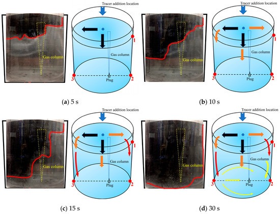
Figure 7.
A typical photo and schematic diagram of tracer transport in the first transport path. (The red line in the physical image on the left is the tracer diffusion profile, and the black, orange, red and yellow arrows in the schematic diagram on the right represent the transport changes of the tracer in four time intervals of 5s, 10s, 15s and 30s. The red dots and numbers represent the three monitoring points and their locations).
The dimensionless concentration curves (abbreviated as DCC in the later sections) at three monitoring points in the first transport path of the tracer are shown in Figure 8. At 6 s, the tracer reached the right wall of the ladle. A portion of the tracer reached monitoring point 1, and the DCC peaked at 1.3 at about 12 s. Subsequently, the DCC at monitoring point 1 began to decline and the tracer concentration rapidly decreased to approach 0 at 28 s. This indicates that the tracer began to transport downward and that no tracer continued to reach monitoring point 1. The tracer arrived at monitoring point 2 at 17 s, and the DCC showed a parabolic type. The tracer concentration at monitoring point 2 initially increased and then decreased, followed by a rapid increase after 52 s. The reason why the DCC at monitoring point 2 first increased and then decreased is because a small portion of the tracer was transported downward from the right wall to the bottom, and the transport of the tracer to point 2 was not continuous. From the DCC at monitoring point 3, it can be seen that the tracer reached the bottom of the left side of the ladle at 18 s. The dimensionless concentration value of the curve increased rapidly, and its peak value was around 5, indicating that an extremely large portion of tracers reached the bottom of the left side of the ladle. As the curve gradually declined, the concentration at this point approached the average concentration during homogenization at around 110 s. This indicates that there are tracers staying at the bottom of the left wall and that there is an inactive area in the ladle.
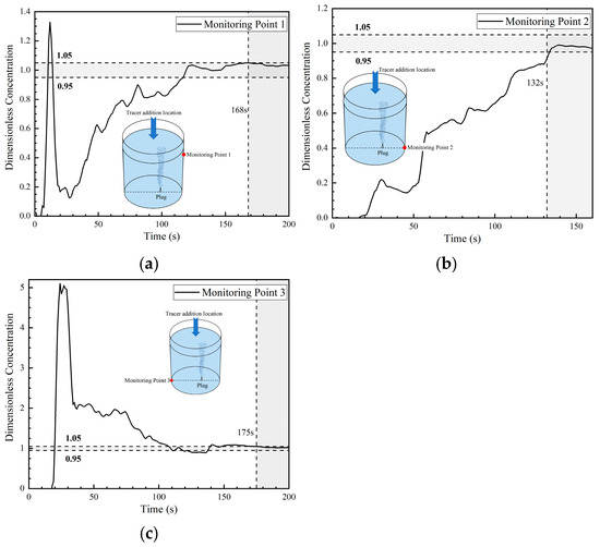
Figure 8.
Dimensionless concentration curve at each monitoring point of ladle in the first transport path: (a) monitoring point 1; (b) monitoring point 2; and (c) monitoring point 3.
The DCC at monitoring point 1 rose rapidly again at 28 s because the tracer of the first circulation flow was brought back to the liquid surface of the ladle by the gas column. At 52–59 s, part of the tracer reached monitoring point 2 through the second circulation flow. Hence, the dimensionless concentration at monitoring point 2 began to rise rapidly, and the mixing at this point was achieved at 132 s. The mixing times at monitoring points 1 and 3 were longer, which were 168 s and 175 s, respectively.
3.2.2. Second Transport Path of the Tracer
Figure 9 is a schematic diagram of the second transport path of the tracer. The tracer was mainly transported on the left side but bifurcated when it was transported downward. Similar to the first transport path, within 5 s after the tracer was added, the tracer was transported onto the free surface of the ladle. The tracer was mainly transported to the left and middle areas of the ladle. During the 5–10 s after the tracer was added, the tracer began to transport to the right wall of the ladle. Compared with the first transport path, the transport of the tracer on the left wall slowed down, and the tracer transport boundary reached half the height of the liquid level. In the first transport path, the downward transport trend in the tracer near the left wall is more obvious. During the 10–15 s after the tracer is added, a portion of the tracer in the middle area began to move to the vicinity of the gas column and slowly passed through the gas column and transported to the right side wall. Compared with the first transport path at the same time, the transport of the tracer on the right side wall was enhanced at this time, and the transport boundary moved further downward. During the 15–30 s after the tracer was added, the tracer was transported and diffused from the left and right side walls of the ladle to the bottom of the ladle, but at 30 s, the tracer had not yet been transported to the middle area of the bottom of the ladle. The tracer in the middle area bifurcated during the downward movement, as shown by the green arrows in Figure 9d. A portion of the tracer was brought back to the free liquid surface under the action of the gas column, and the other portion of the tracer passed through the gas column to the bottom of the right side of the ladle.
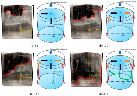
Figure 9.
A typical photo and schematic diagram of tracer transport in the second transport path. (The red line in the physical image on the left is the tracer diffusion profile, and the black, orange, red and yellow arrows in the schematic diagram on the right represent the transport changes of the tracer in four time intervals of 5s, 10s, 15s and 30s. The red dots and numbers represent the three monitoring points and their locations).
Figure 10 shows the dimensionless concentration curves (DCC) at three monitoring points in the second transport path of the tracer. It is similar to the curves of the first transport path. The difference is the curves at monitoring point 1 and 3. At 8 s, the DCC at monitoring point 1 began to increase, and the peak value of the DCC was 0.9. Then, the DCC declined rapidly and maintained a dimensionless concentration value of 0.2 to 0.4 during 20–35 s, which is slightly higher than the concentration value close to 0 in the first transport path. This indicates that the tracer continued to transport to monitoring point 1. Then, the tracer began to transport downward on the right side of the ladle and reached monitoring point 2 at 30 s. The DCC at monitoring point 2 is a parabolic type, which is similar to the curve of monitoring point 2 in the first transport path. However, the dimensionless concentration at monitoring point 2 in this path increased after 40 s, and the concentration value is ranged between 0.4 and 0.5 during 40–80 s. This is due to the fact that a portion of the tracer in the middle of the ladle bifurcated and then transported to the bottom of the right side of the ladle. The DCC at monitoring point 1 rose again at about 35 s, because the tracer of the first circulation flow was brought back to the surface of the ladle by the gas column, which is similar to the result in the first transport path. The time for the tracer on the left to arrive at monitoring point 3 is 36 s, which is slightly later than the time to arrive at the bottom of the right side of the ladle (30 s). The curve at this point also shows a tendency of rapid increase, but the peak value is only 1.5, which is much lower than the peak value at this point in the first transport path. This is due to the weakening of the transport of the tracer to the left side of the ladle in the second transport path. In addition, for the curve at this point, the dimensionless concentration fluctuated between 1.2 and 1.5 during 50–110 s. It indicates that the tracer stayed in this area for a long time and that this area was an inactive zone. The mixing times at monitoring points 1, 2, and 3 in the second transport path are 102 s, 151 s, and 196 s, respectively. Compared with the first path, only the mixing time at monitoring point 1 was shortened.
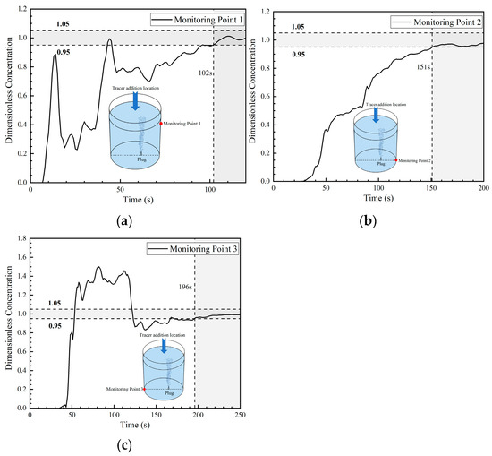
Figure 10.
Dimensionless concentration curve at each monitoring point of ladle: (a) monitoring point 1; (b) monitoring point 2; and (c) monitoring point 3.
3.2.3. Third Transport Path of the Tracer
Figure 11 is a schematic diagram of the third transport path of the tracer. The tracer was mainly transported downward on the left side, but in the middle area, the tracer deviated to the right side when transporting downward. Within 5 s after the tracer was added, the tracer began to transport in three directions at the same time, i.e., left, middle, and right sides. During the 5–10 s after the tracer was added, the tracer on the left side of the ladle transported downward along the left wall. The tracer in the middle region strongly deviated to the right side during the downward transport process, and a small portion of tracer began to transport to the right side along the liquid surface. During the 10–15 s after the tracer was added, the tracer on the left side of the ladle continued to transport downward. The tracer in the middle area continued to disperse to the right. Due to the influence of the gas column, the tracer on the right side of the ladle was transported downward faster than that on the left side. The transport process is indicated by the orange and red arrows in Figure 11b,c. At 15 s, the tracer transport boundary on the right side of the ladle was slightly lower than both the left side and the center of the ladle. In the upper area on the right side of the ladle, there were fewer tracers transported from the surface to the right wall of the ladle. As a result, there was a blank area where the tracer had not been transported near the upper right wall. This inactive area still existed at 30 s. During 15–30 s, the tracer was slowly diffused from both the left and the right side walls to the bottom of the ladle, as indicated by the green arrows in Figure 11d. A key feature of the tracer’s transport in this path is that the concentration/portion of the tracer in the middle region deviating transport to the right side is higher than those of the second transport path.
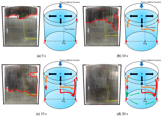
Figure 11.
A typical photo and schematic diagram of tracer transport in the third transport path. (The red line in the physical image on the left is the tracer diffusion profile, and the black, orange, red and yellow arrows in the schematic diagram on the right represent the transport changes of the tracer in four time intervals of 5s, 10s, 15s and 30s. The red dots and numbers represent the three monitoring points and their locations).
Figure 12 presents the dimensionless concentration curves (DCC) at three monitoring points in the third transport path of the tracer. The dimensionless concentration at monitoring point 1 showed a rapid growth trend (at 4 s), and the peak concentration was relatively high (close to 3). Meanwhile, the peak concentration of the curves at the same point 1 in the first two paths were 1.3 and less than 1, respectively. The concentration curve dropped sharply after reaching the peak, showing a sinusoidal type curve. The DCC of the tracer at monitoring point 1 approached 0 at 20 s, which is similar to the results of the first transport path. Later, at about 30 s, the concentration curve started to increase until the final mixing was achieved. A key feature that differs from the first two transport paths is the rapid growth and drops of the curve, which is similar to the pulse signal. This is due to the enhanced transport of the tracer to the right side of ladle. Furthermore, there is no tracer that continued to reach monitoring point 1. This phenomenon is very obvious in Figure 11b.
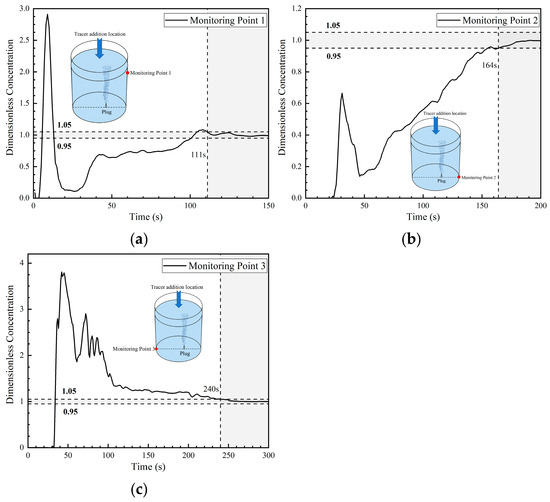
Figure 12.
Dimensionless concentration curve at each monitoring point of the ladle in the third transport path: (a) monitoring point 1; (b) monitoring point 2; (c) monitoring point 3.
The tracer arrived at monitoring point 2 at 23 s, and the concentration curve began to rise sharply, which is totally different from the slowly increasing parabolic type curves of the first two paths. The peak value of the concentration curve at monitoring point 2 is small (about 0.6), but compared with the first two paths, the tracer concentration increased significantly at 23 s, which is due to the deviation of the tracer in the middle area to the right when it was transported downward.
The time when the tracer arrived at monitoring point 3 was 31 s, which is slightly later than the time when it arrived at monitoring point 2. This is because the transport rate of the tracer on the right side was faster than that on the left side. The tracer concentration at monitoring point 3 rose sharply and reached a peak value (close to 3.8) at 40 s. A key feature of the DCC at monitoring point 3 is that the curve presented a sinusoidal oscillation curve type, and there were multiple oscillations during the decreasing process. There is no obvious oscillation behavior for the curves in the first two transport paths. This may be due to the fact that the tracer at the center was periodically brought to the liquid surface by the gas column and transported to the left side of the ladle.
The concentration curve at monitoring point 1 rose again at about 30 s, which is close to the time when the concentration curve at monitoring point 1 rose again in the first two paths, because the tracer was brought back to the liquid surface by the gas column. Compared with the first two paths, the tracer concentration curve rose more slowly, which is due to the fact that the tracer transport from the liquid surface to the upper part of right side of the ladle was weaker. The concentration curve at monitoring point 2 rose again at about 50 s, which is similar to the slow increasing parabolic type curve at this point in the first two paths. The concentration curve at monitoring point 3 began to oscillate at 60 s, and the peak value of the tracer concentration fluctuated between 2 and 2.8. In general, the concentration at monitoring point 3 was higher than the concentration at this point in the second transport path. This indicates that the tracer stayed in this area for a long time, and this area is an inactive area. Overall, the tracer has a strong tendency to be transported to the left side of the ladle in the third transport path. The mixing time at monitoring points 1, 2, and 3 in the third transport path are 111 s, 164 s, and 240 s, respectively. The mixing time at three points are longer than the mixing time at each point in the second transport path. Except for monitoring point 1, the mixing time of the other monitoring points are all longer than those of the first transport path. Among them, the mixing time at monitoring point 3 increases significantly compared with the other two paths.
3.2.4. Fourth Transport Path of the Tracer
Figure 13 is a schematic diagram of the fourth transport path of the tracer. The tracer was mainly transported downward from the left, middle, and right sides with similar intensity at the same time. Within 5 s after the tracer was added, the tracer began to transport in three directions at the same time. During the 5–10 s after the tracer was added, the tracer began to transport to the bottom of the ladle. The overall transport process of the tracer is shown by the orange arrows in Figure 13b. At 10 s, the tracer transport boundary on the right side of the ladle was slightly lower than that at the left and center positions of the ladle. During 10–15 s, the tracer was uniformly transported downward. Compared with the first and second transport paths, the tracer on the right side of the ladle was transported downward faster. At 15 s, the tracer transport boundary on the right side of the ladle was at the same height with the boundary at the center of the ladle, slightly lower than the boundary position on the left side of the ladle. During the 15–30 s after the tracer was added, the tracer transports downwards from both the left, center and right side, and reached the bottom of the ladle at 30 s.
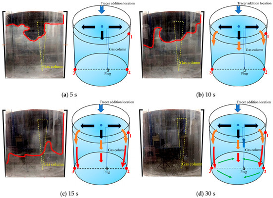
Figure 13.
A typical photo and schematic diagram of tracer transport in the fourth transport path. (The red line in the physical image on the left is the tracer diffusion profile, and the black, orange, red and yellow arrows in the schematic diagram on the right represent the transport changes of the tracer in four time intervals of 5s, 10s, 15s and 30s. The red dots and numbers represent the three monitoring points and their locations).
Figure 14 shows the DCC at three monitoring points in the fourth transport path of the tracer. The DCC at monitoring point 1 presents a step increase tendency that started at 6 s, and the peak concentration is relatively high (close to 4). This indicates that a large portion of tracers arrived at monitoring point 1 during that time period. In addition, the concentration curve oscillates many times and shows a sinusoidal type. This is completely different from the curves in the first two paths, which increased slightly and then decreased sharply. This is due to the enhanced transport of the tracer on the right side of the ladle. In addition, its peak concentration is greater than the peak concentration in the third transport path. It was also noted that the tendency of the tracer concentration at monitoring point 1 in the first three paths to decrease rapidly to about 0 was not observed in this fourth path.
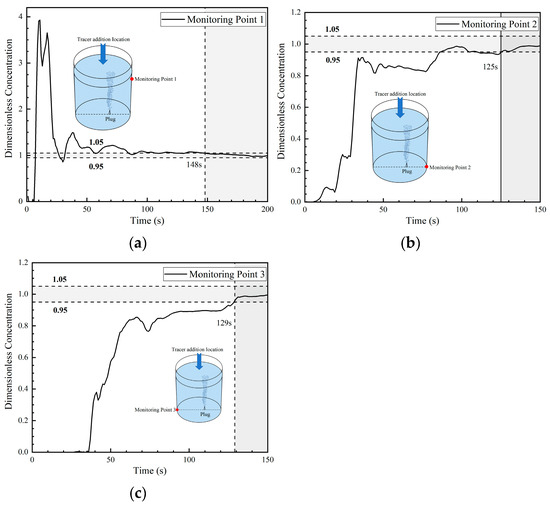
Figure 14.
Dimensionless concentration curve at each monitoring point of the ladle in the fourth transport path: (a) monitoring point 1; (b) monitoring point 2; and (c) monitoring point 3.
The DCC at monitoring point 2 shows a trend in step increase, and the concentration increased sharply at about 20 s, maintaining a peak value of about 0.8 for nearly 90 s, which is higher than the concentration at monitoring point 2 in the first three transport paths. The trend in tracer transport on the right side of the ladle is enhanced compared with the first three paths.
The DCC at monitoring point 3 shows a slowly increasing parabolic type. The concentration slowly increased at about 36 s, and the concentration at this point was always lower than the average concentration, which is significantly different from the rapid increasing type of the first and third transport paths.
From the changes in tracer concentration at the three monitoring points, the transport of tracers to the right side of the ladle (whether on the surface or at the bottom) in the fourth transport path increased significantly. The mixing times at the fourth transport path monitoring points 1, 2, and 3 are 148 s, 125 s, and 129 s, respectively. Among them, the mixing time at monitoring point 3 was significantly shortened compared with that in the first three paths, and the area of the left bottom was no longer the inactive area. Additionally, the mixing time at monitoring point 2 was also shortened.
3.2.5. Fifth Transport Path of the Tracer
Figure 15 is a schematic diagram of the fifth transport path of the tracer. Unlike the previous four paths, the tracer was mainly transported on the right side, and a large portion of the tracer formed a new circulation flow on the right side of the ladle due to the influence of the gas column. In this case, the gas plume oscillated to the right side when injecting the tracer, and this action is shown in Figure 15a. Within 5 s after the tracer was added, a small portion of the tracer was dispersed to the left side along the surface, and a large portion of the tracer was transported from the center area to the direction of the gas column. During the 5–10 s after the tracer was added, the tracer on the left was transported slowly. The tracer in the middle area was rapidly transported to the right side. At 10 s, the transport boundary of the tracer on the right was much lower than that on the left. During the 10–15 s after the tracer was added, a clockwise circulation flow was formed on the right side driven by the gas column. The tracer on the left continued to transport downward, but the transport rate was extremely slow. Its transport boundary was still adjacent to the top of the liquid level. During the 15–30 s after the tracer was added, the tracers in the center and right areas transported downwards as indicated by the green arrows in Figure 15d. And the tracers reached the bottom at 30 s. However, the tracers in the left area were close to the bottom but have not completely reached the bottom of the left side of the ladle.
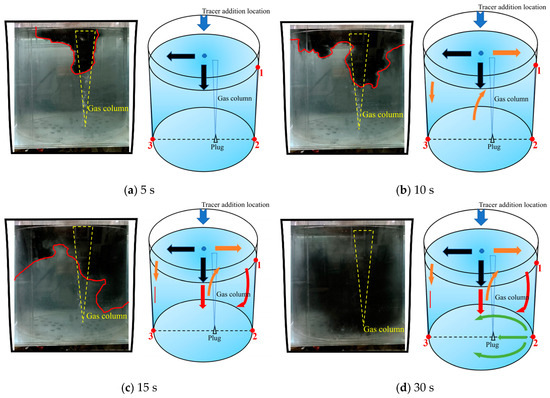
Figure 15.
A typical photo and schematic diagram of tracer transport in the fifth transport path. (The red line in the physical image on the left is the tracer diffusion profile, and the black, orange, red and yellow arrows in the schematic diagram on the right represent the transport changes of the tracer in four time intervals of 5 s, 10 s, 15 s and 30 s. The red dots and numbers represent the three monitoring points and their locations).
Figure 16 presents the DCC at three monitoring points in the fifth transport path of the tracer. The DCC at monitoring point 1 shows a rapid increasing tendency, and its concentration curve peak value is 8.2, which is much higher than the peak concentration at monitoring point 1 of all the first four transport paths. Then, the dimensionless concentration at monitoring point 1 dropped sharply and approached 0 at 28 s. At this time, a large portion of tracers left monitoring point 1 and were transported to the bottom of the ladle. The curve change tendency is somehow similar to that of the third path.
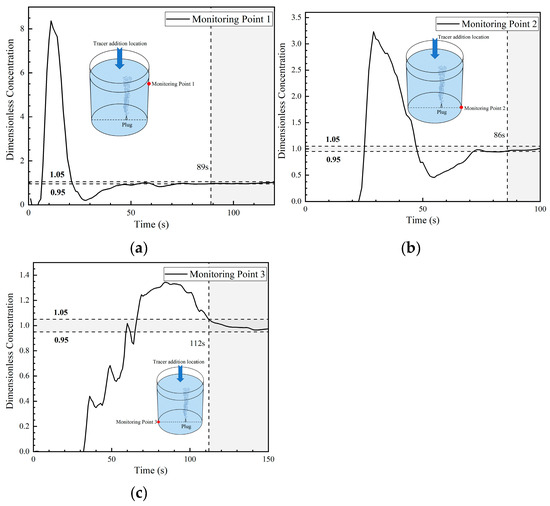
Figure 16.
Dimensionless concentration curve at each monitoring point of ladle in the fifth transport path: (a) monitoring point 1; (b) monitoring point 2; and (c) monitoring point 3.
At 22 s, the tracer arrives at monitoring point 2, showing a step increase tendency and reaching a peak value (close to 3.2) at 30 s. The DCC at monitoring point 2 presents a sinusoidal type, which is completely different from the DCC (parabolic type) at monitoring point 2 in the first four transport paths. As shown in Figure 15b–d, a large portion of tracers were quickly transported to monitoring point 2, and the tracers were mainly transported on the right side of the ladle.
The tracer arrived at monitoring point 3 at 32 s, which was 10 s later than the time it arrived at monitoring point 2. The concentration curve at monitoring point 3 shows three intermittent increases and maintains a peak value of about 1.3 during 65 s to 100 s. In the first four transport paths, the concentration curves at monitoring point 3 changed slightly during a short period of time, indicating that the tracer stayed in this area for a long time and this area was an inactive area. Judging from the peak values of the concentration curves of all the five transport paths, the peak values of the concentration curves at monitoring point 3 of the fourth and fifth transport paths were smaller than those of the first three paths, indicating that the tracer transport on the left side of the ladle was weaker. The mixing time of the three monitoring points in the fifth path are 89 s, 86 s, and 112 s, respectively, which are significantly lower than the mixing time in the other four paths.
3.3. Analysis of Mixing Time of Five Transport Paths
3.3.1. Analysis of Mixing Time at Each Monitoring Point in Five Transport Paths
Figure 17a–c shows the comparison of the mixing time in different transport paths at three monitoring points, respectively. The horizontal dotted line is the average mixing time at the same monitoring point of the five transport paths. As shown in Figure 15a, the mixing time at monitoring point 1 is 123 s, and the maximum and minimum values are 168 s and 89 s, respectively. The difference between the mixing time and the average mixing time at monitoring point 1 in the first, second, fourth, and fifth transport paths are 45 s, 21 s, 25 s, and 34 s, respectively. In the third transport path, the mixing time differs from the average mixing time by only 12 s, making it the path with the smallest mixing time deviation among the five paths.
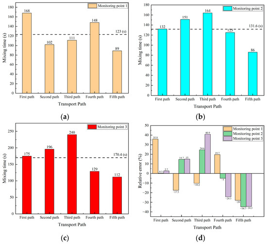
Figure 17.
Comparison of mixing time and error in five transport paths. (a) Mixing time at monitoring point 1; (b) mixing time at monitoring point 2; (c) mixing time at monitoring point 3; and (d) relative error of mixing time at each monitoring point.
As shown in Figure 17b, the mixing time at monitoring point 2 for different transport paths has an average of 131.6 s, with the maximum and minimum values as 164 s and 86 s, respectively. The difference between the mixing time and the average mixing time in the second, third, and fifth transport paths are 19.4 s, 32.4 s, and 45.6 s, respectively. This difference in the first transport path and the fourth transport path are 0.4 s and 6.6 s, respectively, and those mixing time differences are less than 10 s.
As shown in Figure 17c, the mixing time at monitoring point 3 for the five different transport paths has an average of 170.4 s. The mixing time at this point is significantly higher than that at the other two monitoring points, with a maximum value of 240 s and a minimum value of 112 s, resulting in a difference in more than twofold. The differences between the mixing time and the average mixing time for the second, third, fourth, and fifth transport paths are 25.6 s, 69.6 s, 41.4 s, and 58.4 s, respectively. In contrast, the mixing time for the first transport path differs from the average by only 4.6 s.
Figure 17d shows the relative error of the mixing time at the three monitoring points in the five transport paths. In the first transport path, the relative error of the mixing time at monitoring point 1 is 35.9%, while the relative errors of the mixing time at monitoring points 2 and 3 are only 0.3% and 2.7%, respectively. The mixing time values at monitoring points 2 and 3 in this path are closest to the average value. In the second transport path, the relative error of the mixing time at the three monitoring points fluctuates around 15%. The relative errors of the mixing time at the three monitoring points in the third transport path are −10.2%, 24.6%, and 40.9%, respectively, among which the relative error of the mixing time at monitoring point 3 is greatest of all the other transport paths. The relative errors of the mixing time at the monitoring points of the fourth transport path are 19.7%, −5%, and −24.3%, respectively. The relative errors of the mixing time at the monitoring points of the fifth transport path are −28%, −34.7%, and −34.3%, respectively, and the relative errors of the mixing time at each monitoring point are around 30%. In summary, the relative errors of the mixing time at the monitoring points in the first, second and fourth transport paths are small, while the relative errors in the third and fifth transport paths are relatively large.
3.3.2. Analysis of Average Mixing Time of Each Transport Path
Figure 18a shows the averaged mixing time at three monitoring points in each transport path. The values are 158.3 s, 149.7 s, 171.7 s, 134 s, and 95.7 s for five typical transport path trails. A simple average value of the above five values is 141.9 s. Among the five different transport paths, the averaged mixing time of the fifth transport path is the smallest mixing time among all transport paths. The averaged mixing time of the third transport path is the largest mixing time among all transport paths. The averaged mixing time for the other three transport paths is close.
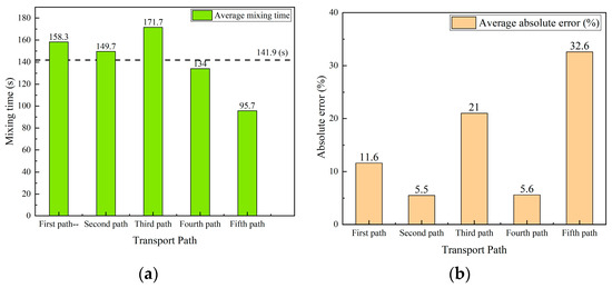
Figure 18.
Comparison of averaged mixing time and error in five transport paths. (a) Average mixing time. (b) Absolute error of averaged mixing time.
A further comparison of the absolute error between the averaged mixing time of each path and the average value 141.9 s are shown in Figure 18b. The results also show that the mixing time deviates significantly for the third and fifth transport path, and the mixing time is close for the other three paths.
4. Discussion
1. As shown in Figure 19, when the tracer is added from the center, there are five transport paths for the tracer. In the first three transport paths, the tracers are mainly transported from the left side and the center downward, and the tracer transport to the right side is less. In the first path, the tracer is mainly transported on the left side. The initial diffused tracer concentration at the right side region of the ladle is low, and the concentration curve in the later period increases slowly in a parabolic type. The mixing time at point 1 is the longest among all paths.
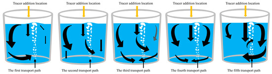
Figure 19.
Schematic diagram of transport paths of the tracer. (The black arrows represent the direction of tracer transport, and the size of the arrows represents the intensity of tracer transport).
In the second and third transport paths, the tracer transport forms a bifurcation when it is transported downward from the center. The tracer transport portion/intensity to the right side in the second transport path is lower than that in the third transport path. In the third transport path, the center downward transport stream is strong, the tracer in the center is brought to the liquid surface by the gas column, and the overall transport of tracers to the left side of the ladle is enhanced. In the first three paths, the tracer concentration that transported to the left side of the ladle is higher, and a “dead zone” is formed at the bottom of the left side of the ladle. As a result, the mixing time at monitoring point 3 is longer. In the third path, the tracer initially transports more strongly to the bottom right side of the ladle, while the transport to the top right side is weaker. In the subsequent stage, few tracers continue to reach the top and bottom at the right side, and the mixing time of monitoring point 2 at the bottom right is the longest among all paths.
In the fourth transport path, the tracer is mainly transported downward from the left, middle, and right sides with similar intensity at the same time. The tracer concentrations transported to the left and right sides are equal, and the mixing time at each monitoring point is reduced.
In the fifth transport path, a significant difference from the other paths is that the tracer is mainly transported from the center to the right. The gas plume oscillates to the right side and the tracer flows toward the gas column in the right side direction. Due to the action of the gas column, the tracer forms a clockwise circulation flow on the right. The downward flow of the tracer in the central is mixed by the rising gas column, leading to a better overall mixing. The mixing time at each monitoring point is significantly reduced, with the mixing time at monitoring point 3 being only half of the maximum mixing time observed at this point of all the paths.
There are two cases where the mixing time is long. One case is when the concentration curve at the monitoring point is a slow increasing parabolic type, and few tracers continue to reach this point at the subsequent stage, such as point 1 in the first path and point 2 in the third path. Another case is that the bottom monitoring points with a high initial concentration and accumulation of tracers, has a slow tracer diffusion and transport process, such as monitoring point 3 in the first three paths.
2. There are errors in the measured mixing time at each monitoring point in the five transport paths of the tracer. In the first transport path, only the error at monitoring point 1 (error of 35.9%) is large, and the errors at monitoring points 2 and 3 are very small. The error at monitoring point 3 in the third transport path (error of 40.9%) is the largest error among all monitoring points, and the errors at the other two monitoring points are less than 30%. The errors of the three monitoring points in the fifth transport path are relatively large, and the mixing time errors at monitoring points 2 and 3 are more than 30%. From the averaged mixing time of the three monitoring points in the five transport paths of the tracer (as shown in Figure 16), the errors of the second and fourth transport paths are the smallest (about 5.5%), and the maximum error is the fifth transport path (32.6%). The error of the first transport path is caused by a high tracer concentration on the left side of the ladle and the low tracer concentration on the right side at the beginning of the transport. Furthermore, the large error of the third transport path is due to the accumulation of tracers at the bottom of the left and right sides of the ladle, which increased the mixing time. In addition, the reason for the large error in the fifth transport path is that the transport rate of a large portion of tracers is accelerated due to the action of the gas column, and the mixing time at the monitoring point is the shortest among all the other transport paths.
The numerical simulation results revealed that the transport of the tracer is only identical to the first transport path. This difference is because numerical simulation requires assumptions and simplifications of the basic theories, and the accuracy of the simulation results depends on the accuracy of the model and parameters. However, the results of the water model experiment are influenced by many practical factors, e.g., the initial velocity of the tracer after it is added. This effect is more pronounced under low gas flow rate conditions, as the various paths described in this study.
3. Li et al. [117] studied the tracer transport and mixing process under moderate gas flow rate conditions, and they found two trends in concentration curves at the monitoring point that were located at the bottom of right side of ladle (corresponding to point 2 in this study), namely Trend 1 (sinusoidal type) and Trend 2 (parabolic type). When the tracers flow vertically downward and shift towards the gas column side, such as the fifth transport path studied in this paper, a sinusoidal type curve will appear. When the tracer is transported asymmetrically, i.e., it moves downward along the left side of the ladle following the main circulation flow, a parabolic type curve will appear. In this study, parabolic curves were also found in the first two transport paths, in which the flow is dominated by left-side circulation flow. Unlike the results observed under moderate gas flow rates, in the third transport path of this study, a portion of the tracer preferentially reaches the bottom of the right side of the ladle. At the subsequent stages, few tracers continue to reach the bottom right side. Thus, the concentration curve shows a small peak at the first stage, followed by a parabolic-shaped curve. Whereas in the study by Li et al. [117], the concentration curves at the monitoring point at the left bottom of the ladle were relatively consistent, i.e., they were all parabolic curves, and they increased rapidly at around 35 s. For the transport path dominated by the left circulation flow in this study, the curves at this point also showed the characteristics of rapid increase. Only in the fourth and fifth transport paths, the curve at this point showed a parabolic or lower peak concentration growth type. This also indicates that when the flow rate is small, the salt solution tracer has a greater impact on the flow field, and the diversity of its transport process is significant.
5. Conclusions
This paper studied the transport process and the mixing time of salt solution tracer in a water model of a gas-stirred ladle with a low gas flow rate. After a large number of repeated experiments, the different transport paths of the tracer and the error of the mixing time in each transport path were discussed and compared with the numerical simulation results. The conclusions are as follows:
- The results of a large number of repeated experiments on the water model show that there are five transport paths for the tracer in the ladle. The tracer of the first path was mainly transported by the left-side main circulation flow, and the tracer began to transport to the right side after it was transported to the bottom of the ladle. The tracer of the second and third paths were also mainly transported by the left-side circulation flow, but bifurcations occurred when the tracer in the middle area was transported downward. In the third path, the portion and intensity of the tracer transferring to the right side from the central region was higher than in the second path. The fourth path is that the tracer was transported downward from the left, middle, and right sides with a similar intensity at the same time, and the portions on the left and right sides were close. The fifth path is that the tracer was mainly transported on the right side, and the tracer formed a clockwise circulation flow on the right side due to the influence of the gas column.
- Numerical simulation results show that after the tracer was added, it primarily followed the left-side anticlockwise main circulating flow for transport. Most of the tracer was transported downward along the left side wall, and after reaching the bottom, it started to transport to the right. When passing through the gas column, a portion of the tracer reached the bottom of the right side and gradually transported upward along the right side wall, and the other portion of the tracer was carried to the free surface by the gas column. The numerical simulation results are similar only to the first transport path in the water model results and are significantly different from the other four transport paths.
- The mixing time in the third and fifth transport paths shows the maximum and minimum values among all paths, respectively. The error between the mixing time and the averaged mixing time at each monitoring point in the five transport paths of the tracer is between −34.7% and 40.9%. In particular, the errors of mixing time at each monitoring point in the third and fifth transport paths are relatively large. In addition, the mixing time at monitoring points 2 and 3 in the third transport path is twice that of mixing time at the same monitoring points in the fifth transport path. Furthermore, the error of the averaged mixing time of each path and the path-based average value is between 5.5% and 32.6%, and the errors of the second and fourth transport paths are relatively small, while the errors of the third and fifth transport paths are considerably large.
Author Contributions
Conceptualization, K.Y. and C.C.; methodology, C.C., K.Y., W.L. and X.T.; software, X.T., H.Q., Z.G., J.Y. and K.Y.; validation, X.T., H.Q. and C.C.; formal analysis, X.T., H.Q. and J.Y.; investigation, X.T., H.Q., J.W. and X.W.; resources, C.C., K.Y., Z.G. and W.L.; data curation, H.Q., J.Y., Q.Z. and J.W; writing—original draft preparation, H.Q., X.T. and Z.G.; writing—review and editing, J.W., W.L., K.Y., Z.G. and C.C.; visualization, X.T., H.Q., X.W. and Q.Z.; supervision, K.Y. and C.C.; project administration, C.C., K.Y. and W.L.; funding acquisition, C.C. and W.L. All authors have read and agreed to the published version of the manuscript.
Funding
This research was funded by the Applied Fundamental Research Program of Shanxi Province, grant number 202303021221036; and the Undergraduate Innovation and Entrepreneurship Training Program of Shanxi Province, grant number 20230135.
Data Availability Statement
The data are contained within this article.
Acknowledgments
The anonymous reviewers are acknowledged for their valuable comments. The discussions on the bad repeatability of water model experiments with Jiayong Qiu of Jiangsu University of Science and Technology are acknowledged.
Conflicts of Interest
The authors declare no conflicts of interest.
References
- Szekely, J.; Carlsson, G.; Helle, L. Ladle Metallurgy; Springer: Berlin/Heidelberg, Germany, 1989; pp. 27–71. [Google Scholar]
- Jönsson, P.; Jonsson, L.I. The Use of Fundamental Process Models in Studying Ladle Refining Operations. ISIJ Int. 2001, 41, 1289–1302. [Google Scholar] [CrossRef]
- Xin, Z.; Zhang, J.; Peng, K.; Zhang, J.; Zhang, C.; Liu, Q. Modeling of LF refining process: A review. J. Iron Steel Res. Int. 2024, 31, 289–317. [Google Scholar] [CrossRef]
- Duan, H.; Zhang, L.; Thomas, B.; Conejo, A.N. Fluid Flow, Dissolution, and Mixing Phenomena in Argon-Stirred Steel Ladles. Metall. Mater. Trans. B 2018, 49, 2722–2743. [Google Scholar] [CrossRef]
- Duan, H.; Zhang, L.; Thomas, B.G. Effect of melt superheat and alloy size on the mixing phenomena in argon-stirred steel ladles. Steel Res. Int. 2019, 90, 1800288. [Google Scholar] [CrossRef]
- Yang, R.; Chen, C.; Lin, Y.; Zhao, Y.; Zhao, J.; Zhu, J.; Yang, S. Water model experiment on motion and melting of scarp in gas stirred reactors. Chin. J. Process Eng. 2022, 22, 954–962. [Google Scholar] [CrossRef]
- Zhu, J.J.; Chen, C.; Fan, J.P.; Li, L.B.; Chen, M.; Yang, H.B.; Lin, W.M. Study on motion melting and mixing of ice samples in a water model of ladle. J. Taiyuan Univ. Technol. 2023, 54, 1063–1069. [Google Scholar] [CrossRef]
- Liu, C.; Peng, K.Y.; Wang, Q.; Li, G.Q.; Wang, J.J.; Zhang, L.F. CFD Investigation of Melting Behaviors of Two Alloy Particles During Multiphase Vacuum Refining Process. Metall. Mater. Trans. B 2023, 54, 2174–2187. [Google Scholar] [CrossRef]
- Li, X.; Wang, H.; Tian, J.; Wang, D.; Qu, T.; Hou, D.; Hu, S.; Wu, G. Investigation on the Alloy Mixing and Inclusion Removement through Using a New Slot-Porous Matched Tuyeres. Metals 2023, 13, 667. [Google Scholar] [CrossRef]
- Niu, K.; Feng, W.; Conejo, A.N. Effect of the Nozzle Radial Position and Gas Flow Rate on Mass Transfer during Bottom Gas Injection in Ladles with One Nozzle. Metall. Mater. Trans. B 2022, 53, 1344–1350. [Google Scholar] [CrossRef]
- Ji, S.; Niu, K.; Conejo, A.N. Multiphase modeling of steel-slag mass transfer through distorted interface in bottom-stirred ladle. ISIJ Int. 2024, 64, 52–58. [Google Scholar] [CrossRef]
- Podder, A.; Coley, K.S.; Phillion, A.B. Modeling Study of Steel–Slag–Inclusion Reactions during the Refining of Si–Mn Killed Steel. Steel Res. Int. 2022, 94, 2100831. [Google Scholar] [CrossRef]
- Podder, A.; Coley, K.S.; Phillion, A.B. Simulation of Ladle Refining Reactions in Si–Mn-Killed Steel. Steel Res. Int. 2024, 95, 2300330. [Google Scholar] [CrossRef]
- Niu, K.; Feng, W.; Conejo, A.N.; Ramírez-Argáez, M.A.; Yan, H. 3D CFD Model of Ladle Heat Transfer with Gas Injection. Metall. Mater. Trans. B 2023, 54, 2066–2079. [Google Scholar] [CrossRef]
- Wen, X.; Ren, Y.; Zhang, L. Effect of CaF2 Contents in Slag on Inclusion Absorption in a Bearing Steel. Steel Res. Int. 2022, 94, 2200218. [Google Scholar] [CrossRef]
- Li, X.; Hu, S.; Wang, D.; Qu, T.; Wu, G.; Zhang, P.; Quan, Q.; Zhou, X.; Zhang, Z. Inclusion Removements in a Bottom-Stirring Ladle with Novel Slot-Porous Matched Dual Plugs. Metals 2022, 12, 162. [Google Scholar] [CrossRef]
- Sun, Y.; Duan, H.; Zhang, L. A boundary layer model for capture of inclusions by steel–slag interface in a turbulent flow. J. Iron Steel Res. Int. 2023, 30, 1101–1108. [Google Scholar] [CrossRef]
- Cao, J.Q.; Li, Y.; Lin, W.M.; Che, J.L.; Zhou, F.; Tan, Y.F.; Li, D.L.; Dang, J.; Chen, C. Assessment of Inclusion Removal Ability in Refining Slags Containing Ce2O3. Crystals 2023, 13, 202. [Google Scholar] [CrossRef]
- Zhao, J.; Zhu, H.; Chen, J.; Wang, L.; Yan, X.; Sun, J. Numerical Simulation on the Motion Behavior of Micro-inclusions at the Steel–Slag Interface. Metall. Mater. Trans. B 2024, 55, 1700–1711. [Google Scholar] [CrossRef]
- Tao, X.; Cao, J.; Wang, J.; He, X.; Meng, L.; Guo, Y.; Wang, T.; Li, D.; Fan, J.; Chen, C. Physical Model of Inclusions Removal at Static Steel–Slag Interface. Materials 2024, 17, 2244. [Google Scholar] [CrossRef]
- Zhong, H.; Jiang, M.; Wang, Z.; Zhen, X.; Zhao, H.; Li, T.; Wang, X. Formation and Evolution of Inclusions in AH36 Steel During LF–RH–CC Process: The Influences of Ca-Treatment, Reoxidation, and Solidification. Metall. Mater. Trans. B 2023, 54, 593–601. [Google Scholar] [CrossRef]
- Ocampo Vaca, F.A.; Hernández Bocanegra, C.A.; Ramos Banderas, J.Á.; Herrera-Ortega, M.; López Granados, N.M.; Solorio Díaz, G. Effect of Ladle Shroud Blockage on Flow Dynamics and Cleanliness of Steel in Coupled Ladle–Shroud–Tundish System. Steel Res. Int. 2024, 95, 2300616. [Google Scholar] [CrossRef]
- Conejo, A.N. Physical and Mathematical Modelling of Mass Transfer in Ladles due to Bottom Gas Stirring: A Review. Processes 2020, 8, 750. [Google Scholar] [CrossRef]
- Conejo, A.N. It is, either refining impurities or liquid steel mixing in the ladle furnace, but not both. In Proceedings of the 2023 International Conference on Secondary Refining and Inclusion Controlling (SRIC 2023), Kunming, China, 23–25 August 2023; The Chinese Society for Metals: Kunming, China, 2023; Volume 25. [Google Scholar]
- Xie, Y.; Oeters, F. Experimental studies on the flow velocity of molten metals in a ladle model at centric gas blowing. Steel Res. 1992, 63, 93–104. [Google Scholar] [CrossRef]
- Xie, Y.; Oeters, F. Experimental studies on the bath oscillation during gas blowing into liquids part 1 measurements using a single nozzle. Steel Res. 1992, 63, 227–233. [Google Scholar] [CrossRef]
- Xie, Y.; Oeters, F. Measurements of bubble plume behaviour and flow velocity in gas stirred liquid woods metal with an eccentric nozzle position. Steel Res. 1994, 65, 315–319. [Google Scholar] [CrossRef]
- Zhu, M.; Inomoto, T.; Sawada, I.; Hsiao, T.C. Fluid Flow and Mixing Phenomena in the Ladle Stirred by Argon through Multi-Tuyere. ISIJ Int. 1995, 35, 472–479. [Google Scholar] [CrossRef]
- Jauhiainen, A.; Jonsson, L.; Sheng, D. Modelling of alloy mixing into steel: The influence of porous plug placement in the ladle bottom on the mixing of alloys into steel in a gas-stirred ladle. A comparison made by numerical simulation. Scand. J. Metall. 2001, 30, 242–253. [Google Scholar] [CrossRef]
- Ganguly, S.; Chakraborty, S. Numerical modelling studies of flow and mixing phenomena in gas stirred steel ladles. Ironmak. Steelmak. 2008, 35, 524–530. [Google Scholar] [CrossRef]
- Mazumdar, D.; Guthrie, R.L. The physical and mathematical modelling of gas stirred ladle systems. ISIJ Int. 1995, 35, 1–20. [Google Scholar] [CrossRef]
- Mazumdar, D.; Evans, J.W. Macroscopic Models for Gas Stirred Ladles. ISIJ Int. 2004, 44, 447–461. [Google Scholar] [CrossRef]
- Irons, G.; Senguttuvan, A.; Krishnapisharody, K. Recent Advances in the Fluid Dynamics of Ladle Metallurgy. ISIJ Int. 2015, 55, 1–6. [Google Scholar] [CrossRef][Green Version]
- Szekely, J.; Wang, H.; Kiser, K.M. Flow pattern velocity and turbulence energy measurements and predictions in a water model of an argon-stirred ladle. Metall. Trans. B 1976, 7, 287–295. [Google Scholar] [CrossRef]
- Sahai, Y.; Guthrie, R.I.L. Hydrodynamics of gas stirred melts: Part I. Gas/liquid coupling. Metall. Trans. B 1982, 13, 193–202. [Google Scholar] [CrossRef]
- Szekely, J.; Grevet, H.H.; Kaddah, N.E. Melting Rates in Turbulent Recirculating Flow System. Int. J. Heat Mass Transf. 1984, 27, 1116–1121. [Google Scholar] [CrossRef]
- Mazumdar, D.; Guthrie, R.I. Hydrodynamics of CAS method of alloy additions. Ironmak. Steelmak. 1985, 12, 256–264. [Google Scholar]
- Mazumdar, D.; Guthrie, R.I. Hydrodynamic modeling of some gas injection procedures in ladle metallurgy operations. Metall. Trans. B 1985, 16, 83–90. [Google Scholar] [CrossRef]
- Johansen, S.T.; Engh, T.A. Combined Surface injection and Gas-stirring in Ladles Studied in Water Models. Scand. J. Metall. 1985, 14, 214–223. [Google Scholar]
- Krishna-Murthy, G.G.; Mehrotra, S.P.; Ghosh, A. Experimental investigation of mixing phenomena in a gas stirred liquid bath. Metall. Trans. B 1988, 19, 839–850. [Google Scholar] [CrossRef]
- Johansen, S.T.; Robertson, D.G.; Woje, K.; Engh, T.A. Fluid dynamics in bubble stirred ladles: Part I. experiments. Metall. Trans. B 1988, 19, 745–754. [Google Scholar] [CrossRef]
- Mietz, J.; Oeters, F. Model Experiments on Mixing Phenomena in Gas-stirred Melts. Steel Res. 1988, 59, 52–59. [Google Scholar] [CrossRef]
- Guo, D.; Irons, G.A. Modeling of Gas-Liquid Reactions in Ladle Metallurgy: Part I. Physical Modeling. Metall. Mater. Trans. B 2000, 31, 1447–1455. [Google Scholar] [CrossRef]
- Krishnapisharody, K.; Irons, G.A. An Analysis of Recirculatory Flow in Gas-Stirred Ladles. Steel Res. Int. 2010, 81, 880–885. [Google Scholar] [CrossRef]
- Conejo, A.N.; Kitamura, S.; Maruoka, N.; Kim, S.J. Effects of Top Layer, Nozzle Arrangement, and Gas Flow Rate on Mixing Time in Agitated Ladles by Bottom Gas Injection. Metall. Mater. Trans. B 2013, 44, 914–923. [Google Scholar] [CrossRef]
- Terrazas, M.S.C.; Conejo, A.N. Effect of Nozzle Diameter on Mixing Time During Bottom-Gas Injection in Metallurgical Ladles. Metall. Mater. Trans. B 2014, 45, 711–718. [Google Scholar] [CrossRef]
- Liu, Z.; Li, L.; Li, B. Modeling of gas-steel-slag three-phase flow in ladle metallurgy: Part I. Physical modeling. ISIJ Int. 2017, 57, 1971–1979. [Google Scholar] [CrossRef]
- Jardón-Pérez, L.E.; Amaro-Villeda, A.; Conejo, A.N.; González-Rivera, C.; Ramírez-Argáez, M.A. Optimizing gas stirred ladles by physical modeling and PIV measurements. Mat. Manuf. Process. 2018, 33, 882–890. [Google Scholar] [CrossRef]
- Jardón-Pérez, L.E.; Amaro-Villeda, A.M.; Trápaga-Martínez, G.; González-Rivera, C.; Ramírez-Argáez, M.A. Utilization of the Planar Laser-Induced Fluorescence Technique (PLIF) to Measure Temperature Fields in a Gas-Stirred Ladle. Metall. Mater. Trans. B 2020, 51, 2510–2521. [Google Scholar] [CrossRef]
- Feng, W.; Conejo, A.N. Physical and Numerical Simulation of the Optimum Nozzle Radial Position in Ladles with One Nozzle and Bottom Gas Injection. ISIJ Int. 2022, 62, 1211–1221. [Google Scholar] [CrossRef]
- Conejo, A.N.; Feng, W. Ladle Eye Formation Due to Bottom Gas Injection: A Reassessment of Experimental Data. Metall. Mater. Trans. B 2022, 53, 999–1017. [Google Scholar] [CrossRef]
- Wondrak, T.; Timmel, K.; Bruch, C.; Gardin, P.; Hackl, G.; Lachmund, H.; Lüngen, H.B.; Odenthal, H.J.; Eckert, S. Large-Scale Test Facility for Modeling Bubble Behavior and Liquid Metal Two-Phase Flows in a Steel Ladle. Metall. Mater. Trans. B 2022, 53, 1703–1720. [Google Scholar] [CrossRef]
- Jardón-Pérez, L.E.; Conejo, A.N.; Amaro-Villeda, A.M.; González-Rivera, C.; Ramírez-Argáez, M.A. Analysis of the Effect of Gas Injection System on the Heating Rate of a Gas Stirred Steel Ladle Assisted by Physical Modeling and PIV-PLIF Measurements. ISIJ Int. 2023, 63, 484–491. [Google Scholar] [CrossRef]
- Jojo-Cunningham, Y.; Guo, X.; Zhou, C.; Liu, Y. Volumetric Flow Field inside a Gas Stirred Cylindrical Water Tank. Fluids 2024, 9, 11. [Google Scholar] [CrossRef]
- Szekely, J.; Asai, S. Practical Applications of the Mathematical Representation for Turbulent Recirculatory Flows. Trans. ISIJ 1975, 15, 277–285. [Google Scholar] [CrossRef]
- Nakanishi, K.; Szekely, J. Deoxidation Kinetics in a Turbulent Flow Field. Trans. ISIJ 1975, 15, 522–530. [Google Scholar] [CrossRef]
- Nakanishi, K.; Fujii, T.; Szekely, J. Possible relationship between energy dissipation and agitation in steel processing operations. Ironmak. Steelmak. 1975, 2, 193–197. [Google Scholar]
- Szekely, J.; Lehner, T.; Chang, C.W. Flow phenomena, mixing, and mass transfer in argon-stirred ladles. Ironmak. Steelmak. 1979, 6, 285–293. [Google Scholar]
- Johansen, S.T.; Boysan, F.; Ayers, W.H. Mathematical modelling of bubble driven flows in metallurgical processes. Appl. Sci. Res. 1987, 44, 197–207. [Google Scholar] [CrossRef]
- Johansen, S.T.; Boysan, F. Fluid dynamics in bubble stirred ladles: Part II. Mathematical modelling. Metall. Trans. B 1988, 19, 755–764. [Google Scholar] [CrossRef]
- Zhu, M.; Sawada, I.; Yamasaki, N.; Hsiao, T.C. Numerical Simulation of Three-Dimensional Fluid Flow and Mixing Process in Gas-stirred Ladles. ISIJ Int. 1996, 36, 503–511. [Google Scholar] [CrossRef]
- Guo, D.; Irons, G.A. Modeling of Gas-Liquid Reactions in Ladle Metallurgy: Part II. Numerical Simulation. Metall. Mater. Trans. B 2000, 31, 1457–1464. [Google Scholar] [CrossRef]
- Liu, H.; Qi, Z.; Xu, M. Numerical Simulation of Fluid Flow and Interfacial Behavior in Three-Phase Argon-Stirred Ladles with One Plug and Dual Plugs. Steel Res. Int. 2011, 82, 440–458. [Google Scholar] [CrossRef]
- Lou, W.; Zhu, M. Numerical Simulations of Inclusion Behavior and Mixing Phenomena in Gas-stirred Ladles with Different Arrangement of Tuyeres. ISIJ Int. 2014, 54, 9–18. [Google Scholar] [CrossRef]
- Mazumdar, D.; Dhandapani, P.; Sarvanakumar, R. Modeling and optimisation of gas stirred ladle systems. ISIJ Int. 2017, 57, 286–295. [Google Scholar] [CrossRef]
- Khan, S.; Idrees, M.; Mushtaq, M.U.; Hussain, S. Two Dimensional (2D) Multi-Scale Modeling of Fixed Bed Adsorption Column Using Computational Fluid Dynamics (CFD) Simulation. Arch. Adv. Eng. Sci. 2024, 2, 1–9. [Google Scholar] [CrossRef]
- Hua, C.; Bao, Y.; Wang, M. Multiphysics numerical simulation model and hydraulic model experiments in the argon-stirred ladle. Processes 2022, 10, 1563. [Google Scholar] [CrossRef]
- Tiwari, R.; Girard, B.; Labrecque, C.; Isac, M.M.; Guthrie, R.I.L. CFD Predictions for Mixing Times in an Elliptical Ladle Using Single- and Dual-Plug Configurations. Processes 2023, 11, 1665. [Google Scholar] [CrossRef]
- Nick, R.S.; Teng, L.; Yang, H.; Tilliander, A.; Glaser, B.; Sheng, D.Y.; Jönsson, P.G.; Björkvall, J. Mathematical modelling of novel combined stirring method during the final stage of ladle refining. Ironmak. Steelmak. 2023, 50, 721–733. [Google Scholar] [CrossRef]
- Li, X.; Wang, D.; Tian, J.; Wang, H.; Qu, T.; Hou, D.; Hu, S.; Zhang, Z.; Zhou, X.; Wu, G. Modeling of Bubble Transportation, Expansion, as Well as Adhesion of Inclusions in a Ladle With Different Tuyeres. Metall. Mater. Trans. B 2024, 55, 14–31. [Google Scholar] [CrossRef]
- Mazumdar, D.; Guthrie, R.I. Mixing models for gas stirred metallurgical reactors. Metall. Trans. B 1986, 17, 725–733. [Google Scholar] [CrossRef]
- Mazumdar, D.; Nakajima, H.; Guthrie, R.I. Possible roles of upper slag phases on the fluid dynamics of gas stirred ladles. Metall. Trans. B 1988, 19, 507–511. [Google Scholar] [CrossRef]
- Turkoglu, H.; Farouk, B. Mixing time and liquid circulation rate in steelmaking ladles with vertical gas injection. ISIJ Int. 1991, 31, 1371–1380. [Google Scholar] [CrossRef][Green Version]
- Joo, S.; Guthrie, R.I. Modeling Flows and Mixing in Steelmaking Ladles Designed for Single and Dual Plug Bubbling Operations. Metall. Trans. B 1992, 23, 765–778. [Google Scholar] [CrossRef]
- Mazumdar, D.; Guthrie, R.I. Mixing Times and Correlations for Gas Stirred Ladle Systems. Iron Steelmak. 1999, 26, 89–96. [Google Scholar]
- Mazumdar, D.; Kim, H.B.; Guthrie, R.I. Modelling Criteria for Flow Simulation in Gas Stirred ladles: Experimental Study. Ironmak. Steelmak. 2000, 27, 302–309. [Google Scholar] [CrossRef]
- Mandal, J.; Patil, S.; Madan, M.; Mazumdar, D. Mixing Time and Correlation for Ladles Stirred with Dual Porous Plugs. Metall. Mater. Trans. B 2005, 36, 479–487. [Google Scholar] [CrossRef]
- Madan, M.; Satish, D.; Mazumdar, D. Modeling of Mixing in Ladles Fitted with Dual Plugs. ISIJ Int. 2005, 45, 677–685. [Google Scholar] [CrossRef]
- Chen, M.; Wang, N.; Yao, Y.; Geng, J.; Xiong, K. Optimal Mixing Effect of LF Bottom Blown Stirring by Two Nozzles. Steel Res. Int. 2007, 78, 468–472. [Google Scholar] [CrossRef]
- Geng, D.; Le, H.; He, J. Optimization of Mixing Time in a Ladle with Dual Plugs. Int. J. Miner. Metall. Mater. 2010, 17, 709–714. [Google Scholar] [CrossRef]
- Maldonado-Parra, F.D.; Ramírez-Argáez, M.A.; Conejo, A.N.; González, C. Effect of both radial position and number of porous nozzles on chemical and thermal mixing in an industrial ladle involving two phase flow. ISIJ Int. 2011, 51, 1110–1118. [Google Scholar] [CrossRef]
- Amaro-Villeda, A.M.; Ramirez-Argaez, M.A.; Conejo, A.N. Effect of Slag Properties on Mixing Phenomena in Gas-stirred Ladles by Physical Modeling. ISIJ Int. 2014, 54, 1–8. [Google Scholar] [CrossRef]
- Jardón-Pérez, L.E.; Amaro-Villeda, A.; González-Rivera, C.; Trápaga, G.; Conejo, A.N.; Ramírez-Argáez, M.A. Introducing the Planar Laser-Induced Fluorescence Technique (PLIF) to Measure Mixing Time in Gas-Stirred Ladles. Metall. Mater. Trans. B 2019, 50, 2121–2133. [Google Scholar] [CrossRef]
- González-Bernal, R.; Solorio-Diaz, G.; Ramos-Banderas, A.; Torres-Alonso, E.; Hernández-Bocanegra, C.A.; Zenit, R. Effect of the Fluid-Dynamic Structure on the Mixing Time of a Ladle Furnace. Steel Res. Int. 2018, 89, 1700281. [Google Scholar] [CrossRef]
- Liu, Y.; Bai, H.; Liu, H.; Ersson, M.; Jönsson, P.G.; Gan, Y. Physical and Numerical Modelling on the Mixing Condition in a 50 t Ladle. Metals 2019, 9, 1136. [Google Scholar] [CrossRef]
- Tang, H.; Liu, J.; Zhang, S.; Guo, X.; Zhang, J. A novel dual plugs gas blowing mode for efficient ladle metallurgy. Ironmak. Steelmak. 2019, 46, 405–415. [Google Scholar] [CrossRef]
- Villela-Aguilar, J.D.; Ramos-Banderas, J.A.; Hernández-Bocanegra, C.A.; Urióstegui-Hernández, A.; Solorio-Díaz, G. Optimization of the mixing time using asymmetrical arrays in both gas flow and injection positions in a dual-plug ladle. ISIJ Int. 2020, 60, 1172–1178. [Google Scholar] [CrossRef]
- Herrera-Ortega, M.; Ramos-Banderas, J.Á.; Hernández-Bocanegra, C.A.; Montes-Rodríguez, J.J. Effect of the location of tracer addition in a ladle on the mixing time through physical and numerical modeling. ISIJ Int. 2021, 61, 2185–2192. [Google Scholar] [CrossRef]
- Gajjar, P.; Haas, T.; Owusu, K.B.; Eickhoff, M.; Kowitwarangkul, P.; Pfeifer, H. Physical study of the impact of injector design on mixing, convection and turbulence in ladle metallurgy. Eng. Sci. Technol. Int. J. 2019, 22, 538–547. [Google Scholar] [CrossRef]
- Merder, T.; Warzecha, P.; Pieprzyca, J.; Warzecha, M.; Wende, R.; Hutny, A. Model Investigation of Argon Injection into Liquid Steel at Ladle Furnace Station with Using of Innovative Module. Materials 2023, 16, 7698. [Google Scholar] [CrossRef]
- Li, Z.; Ouyang, W.; Wang, Z.; Zheng, R.; Bao, Y.; Gu, C. Physical Simulation Study on Flow Field Characteristics of Molten Steel in 70t Ladle Bottom Argon Blowing Process. Metals 2023, 13, 639. [Google Scholar] [CrossRef]
- Zhou, X.; Zhang, Y.; He, Q.; Ni, P.; Yue, Q.; Ersson, M. Novel Evaluation Method to Determine the Mixing Time in a Ladle Refining Process. Metall. Mater. Trans. B 2022, 53, 4114–4123. [Google Scholar] [CrossRef]
- Taylor, I.F.; Dang, P.; Schwarz, M.P.; Wright, J.K. An Improved Method for the Experimental Validation of Numerical Mixing Time Predictions. In Proceedings of the 72nd Steelmaking Proceedings, ISS, Chicago, IL, USA, 2–5 April 1989; pp. 505–516. [Google Scholar]
- Mietz, J.; Oeters, F. Mixing Theories for Gas-Stirred Melts. Steel Res. 1987, 58, 446–453. [Google Scholar] [CrossRef]
- Mietz, J.; Oeters, F. Flow Field and Mixing with Eccentric Gas Stirring. Steel Res. 1989, 60, 387–394. [Google Scholar] [CrossRef]
- Mietz, J.; Oeters, F. Model Studies of Mixing Phenomena in Stirred Melts. Can. Metall. Quart. 1989, 28, 19–27. [Google Scholar] [CrossRef]
- Mietz, J.; Schneider, S.; Oeters, F. Model experiments on mass transfer in ladle metallurgy. Steel Res. 1991, 62, 1–9. [Google Scholar] [CrossRef]
- Riabov, D.; Gain, M.M.; Kargul, T.; Volkova, O. Influence of Gas Density and Plug Diameter on Plume Characteristics by Ladle Stirring. Crystals 2021, 11, 475. [Google Scholar] [CrossRef]
- Jardón-Pérez, L.E.; González-Rivera, C.; Ramirez-Argaez, M.A.; Dutta, A. Numerical Modeling of Equal and Differentiated Gas Injection in Ladles: Effect on Mixing Time and Slag Eye. Processes 2020, 8, 917. [Google Scholar] [CrossRef]
- Conejo, A.N.; Zhao, G.; Zhang, L. On the Limits of the Geometric Scale Ratio Using Water Modeling in Ladles. Metall. Mater. Trans. B 2021, 52, 2263–2274. [Google Scholar] [CrossRef]
- Jiang, X.; Cui, Z.; Chen, M.; Zhao, B. Mixing Behaviors in the Horizontal Bath Smelting Furnaces. Metall. Mater. Trans. B 2019, 52, 173–180. [Google Scholar] [CrossRef]
- Aguilar, G.; Solorio-Diaz, G.; Aguilar-Corona, A.; Ramos-Banderas, J.A.; Hernández, C.A.; Saldaña, F. Study of the Effect of a Plug with Torsion Channels on the Mixing Time in a Continuous Casting Ladle Water Model. Metals 2021, 11, 1942. [Google Scholar] [CrossRef]
- Pan, S.; Chiang, J.D.; Hwang, W.S. Effects of gas injection condition on mixing efficiency in the ladle refining process. J. Mater. Eng. Perform. 1997, 6, 113–117. [Google Scholar] [CrossRef]
- Ek, M.; Wu, L.; Valentin, P.; Sichen, D. Effect of Inert Gas Flow Rate on Homogenization and Inclusion Removal in a Gas Stirred Ladle. ISIJ Int. 2010, 81, 1056–1063. [Google Scholar] [CrossRef]
- Tan, F.; He, Z.; Jin, S.; Pan, L.; Li, Y.; Li, B. Physical Modeling Evaluation on Refining Effects of Ladle with Different Purging Plug Designs. Steel Res. Int. 2020, 91, 1900606. [Google Scholar] [CrossRef]
- Chen, C.; Cheng, G.; Sun, H.; Hou, Z.; Wang, X.; Zhang, J. Effects of Salt Tracer Amount, Concentration and Kind on the Fluid Flow Behavior in a Hydrodynamic Model of Continuous Casting Tundish. Steel Res. Int. 2012, 83, 1141–1151. [Google Scholar] [CrossRef]
- Chen, C.; Jonsson, L.I.; Tilliander, A.; Cheng, G.; Jönsson, P. A Mathematical Modeling Study of Tracer Mixing in a Continuous Casting Tundish. Metall. Mater. Trans. B 2015, 46, 169–190. [Google Scholar] [CrossRef]
- Chen, C.; Jonsson, L.I.; Tilliander, A.; Cheng, G.; Jönsson, P. A mathematical modeling study of the influence of small amounts of KCl solution tracers on mixing in water and residence time distribution of tracers in a continuous flow reactor-metallurgical tundishc. Chem. Eng. Sci. 2015, 137, 914–937. [Google Scholar] [CrossRef]
- Ding, C.; Lei, H.; Niu, H.; Zhang, H.; Yang, B.; Li, Q. Effects of Tracer Solute Buoyancy on Flow Behavior in a Single-Strand Tundish. Metall. Mater. Trans. B 2021, 52, 3788–3804. [Google Scholar] [CrossRef]
- Ding, C.; Lei, H.; Niu, H.; Zhang, H.; Yang, B.; Zhao, Y. Effects of Salt Tracer Volume and Concentration on Residence Time Distribution Curves for Characterization of Liquid Steel Behavior in Metallurgical Tundish. Metals 2021, 11, 430. [Google Scholar] [CrossRef]
- Zhang, Y.; Chen, C.; Lin, W.; Yu, Y.; E, D.; Wang, S. Numerical Simulation of Tracers Transport Process in Water Model of a Vacuum Refining Unit: Single Snorkel Refining Furnace. Steel Res. Int. 2020, 91, 202000022. [Google Scholar] [CrossRef]
- Ouyang, X.; Lin, W.; Luo, Y.; Zhang, Y.; Fan, J.; Chen, C.; Cheng, G. Effect of Salt Tracer Dosages on the Mixing Process in the Water Model of a Single Snorkel Refining Furnace. Metals 2022, 12, 1948. [Google Scholar] [CrossRef]
- Xu, Z.; Ouyang, X.; Chen, C.; Li, Y.; Wang, T.; Ren, R.; Yang, M.; Zhao, Y.; Xue, L.; Wang, J. Numerical Simulation of the Density Effect on the Macroscopic Transport Process of Tracer in the Ruhrstahl–Heraeus (RH) Vacuum Degasser. Sustainability 2024, 16, 3923. [Google Scholar] [CrossRef]
- Chen, C.; Rui, Q.; Cheng, G. Effect of Salt Tracer Amount on the Mixing Time Measurement in a Hydrodynamic Model of Gas-Stirred Ladle System. Steel Res. Int. 2013, 84, 900–907. [Google Scholar] [CrossRef]
- Gómez, A.S.; Conejo, A.N.; Zenit, V.R. Effect of Separation Angle and Nozzle Radial Position on Mixing Time in Ladles with Two Nozzles. J. Appl. Fluid Mec. 2018, 11, 11–20. [Google Scholar] [CrossRef]
- Zhang, D.; Chen, C.; Zhang, Y.; Wang, S. Numerical Simulation of Tracer Transport Process in Water Model of Gas-stirred Ladle. J. Taiyuan Univ. Technol. 2020, 51, 50–58. [Google Scholar] [CrossRef]
- Li, L.; Chen, C.; Tao, X.; Qi, H.; Liu, T.; Yan, Q.; Deng, F.; Allayev, A.; Lin, W.; Wang, J. Effect of Salt Solution Tracer Dosage on the Transport and Mixing of Tracer in a Water Model of Asymmetrical Gas-Stirred Ladle with a Moderate Gas Flowrate. Symmetry 2024, 16, 619. [Google Scholar] [CrossRef]
- Krishnapisharody, K.; Irons, G.A. A critical review of the modified Froude number in Ladle Metallurgy. Metall. Mater. Trans. B 2013, 44, 1486–1498. [Google Scholar] [CrossRef]
- Zhan, Z.; Qiu, S.; Yin, S. Study on Water model for 135t LF ladle bottom blowing argon process. Hot Work. Technol. 2017, 46, 98–101. [Google Scholar] [CrossRef]
- Wang, D.M. Modelling of Bubbly Flow in a Sudden Pipe Expansion, Technical Report, BRITE/EURAM II (BE 4098), II-34. 1994.
- Lou, W.; Zhu, M. Numerical Simulation of Gas and Liquid Two-Phase Flow in Gas-Stirred Systems Based on Euler–Euler Approach. Metall. Mater. Trans. B 2013, 44, 1251–1263. [Google Scholar] [CrossRef]
- Wolfshtein, M. The velocity and temperature distribution in one-dimensional flow with turbulence augmentation and pressure gradient. Int. J. Heat Mass Transf. 1969, 12, 301–318. [Google Scholar] [CrossRef]
- Fan, J.; Li, Y.; Chen, C.; Ouyang, X.; Wang, T.; Lin, W. Effect of Uniform and Non-Uniform Increasing Casting Flow Rate on Dispersion and Outflow Percentage of Tracers in Four Strand Tundishes under Strand Blockage Conditions. Metals 2022, 12, 1016. [Google Scholar] [CrossRef]
- Ilegbusi, O.J.; Iguchi, M.; Nakajima, K.; Sano, M.; Sakamoto, M. Modeling Mean Flow and Turbulence Characteristics in Gas Agitated Bath with Top Layer. Metall. Mater. Trans. B 1998, 29, 211–222. [Google Scholar] [CrossRef]
- Siemens. STAR-CCM+ Version 13.04 User Guide; Siemens PLM Software: Munich, Germany, 2019. [Google Scholar]
- Ramírez-López, A. Analysis of Mixing Efficiency in a Stirred Reactor Using Computational Fluid Dynamics. Symmetry 2024, 16, 237. [Google Scholar] [CrossRef]
- Ramírez-López, A.A. Analysis of the Hydrodynamics Behavior Inside a Stirred Reactor for Lead Recycling. Fluids 2023, 8, 268. [Google Scholar] [CrossRef]


Disclaimer/Publisher’s Note: The statements, opinions and data contained in all publications are solely those of the individual author(s) and contributor(s) and not of MDPI and/or the editor(s). MDPI and/or the editor(s) disclaim responsibility for any injury to people or property resulting from any ideas, methods, instructions or products referred to in the content. |
© 2024 by the authors. Licensee MDPI, Basel, Switzerland. This article is an open access article distributed under the terms and conditions of the Creative Commons Attribution (CC BY) license (https://creativecommons.org/licenses/by/4.0/).