Calibrating the Digital Twin of a Laboratory Ball Mill for Copper Ore Milling: Integrating Computer Vision and Discrete Element Method and Smoothed Particle Hydrodynamics (DEM-SPH) Simulations

Abstract

This article presents a novel approach to calibrating the digital twin of a laboratory mill used for copper ore milling. By integrating computer vision techniques for real-time data extraction and employing DualSPHysics simulations for various milling scenarios, including balls only, balls with ore, and balls with slurry, we achieve a high degree of accuracy in matching the digital twin’s behavior with actual mill operations. The calibration process is detailed for mills with three different diameters, highlighting the adjustments in simulation parameters necessary to account for the absence of ore. Understanding the dynamics between the suspension within the mill and the operation of the grinders is crucial for the future improvement of the grinding process. This knowledge paves the way for optimizing the process, not only in terms of the quality of the end product but primarily in terms of energy efficiency. A profound understanding of these interactions will enable engineers and technologists to design mills and grinding processes in a way that maximizes efficiency while minimizing energy consumption.

1. Introduction

The mineral processing industry, a prominent element of modern industrial economies, is crucial for extracting valuable minerals from ores [1]. This fundamental sector transforms raw, naturally occurring materials into useful products, such as metals, which find essential applications in numerous sectors, including construction, automotive, and electronics [2]. In most mineral processing systems, grinding is the one of the first stages, enabling better extraction of valuable components [3], increasing process efficiency, and optimizing energy consumption in subsequent stages of production. In this context, ball mills, integral to mineral extraction and refinement, are central to the fine grinding of ores [4], and the efficacy and efficiency of mineral processing are deeply tied to their performance [5,6].

Despite the simple construction of ball mills and their operation, the grinding process entails a lot of technological challenges. The majority of research efforts and optimization actions are focused on increasing the efficiency of comminution by achieving the proper size reduction in grains [7] with the lowest energy expenditure possible [8]. A particular one is the prediction of mill load behavior, which consists of a mixture of ore particles, water, and grinding media, especially during wet milling. Wet grinding is exceptionally popular in ore processing [9] due to its ability to control the viscosity of the slurry [10], reduce energy consumption and oxidation of certain minerals [11], improve separation [12], and provide control over particle size [13]. The behavior of the mixture, governed by a complex interaction between the liquid, gas, and solid phases inside the mill, is hard to predict [14]. Furthermore, the slurry level in AG/SAG and ball mills significantly influences their power consumption [15].

Contributing to this understanding, ref. [16] conducted a study on the discharge of finer rock, pebbles, ball scraps, and slurry from mills. They demonstrated these elements’ effects on overflow ball mills’ performance. They combined the Discrete Element Method (DEM) and Smoothed Particle Hydrodynamics (SPH) to model the coarser rock components, grinding media, and slurry components. Their modeling yielded valuable data for understanding and optimizing designs for improved performance and wear life. Similarly, ref. [17] suggested a computational approach that combines the Discrete Element Method (DEM) for modeling the solid particles and a continuum description (CFD) for fluid dynamics in a three-phase model. This approach highlights the usefulness of modeling both charge and slurry dynamics. Moreover, their model considered the effect of drag force on slurry movement evoked by particle motion.

In the field, further advancements include studies on the influence of mill speed, slurry concentration, and slurry filling on the impact forces within the mill and the role of slurry pool formation on mill power draw. Refs. [18,19] used an instrumented ball to measure the charge physical quantities in a ball mill, uncovering complex behavior under different mill speeds and slurry filling levels. In a more recent study, Ref. [20] examined the impact of slurry mass concentration on the grinding characteristics of magnetite using ceramic grinding media, leading to significant energy savings and a reduced chance of over-grinding, especially at high concentrations. Further complementing these insights, Ref. [21] underlined the need to accurately simulate the ore milling process that accounts for the unique shapes of ore particles and grinding media. They proposed a polyhedron-sphere contact model based on the “deepest point method” tested through experiments and simulation studies. They found that their model could lead to increased power consumption, enhanced energy utilization efficiency, and substantial collision energy between the ore and the liner, increasing liner wear.

Moreover, Ref. [22] conducted extensive experimental work to clarify granular flow behavior inside a rotating drum. However, most of these studies involved spherical or nearly spherical particles. The impact of non-spherical particles, such as pharmaceutical tablets suitable as tracer particles, on the velocity profile, residence time, and segregation patterns showed significant deviations from those predicted for spherical particles. In particular, non-spherical particles with an aspect ratio greater than two showed considerable differences, including unexpected core segregation patterns and a lower axial dispersion coefficient.

In other research, Ref. [23] demonstrated the difficulty in modeling multifrequency signals like mechanical vibration and acoustic signals from a wet ball mill during the mineral grinding process. They used the empirical mode decomposition (EMD) technique to decompose these signals into multiscale intrinsic mode functions (IMFs) and developed a new adaptive multiscale spectral features selection approach. Their approach allowed the effective modeling of mill load parameters based on shell vibration and acoustic signals. It provided a practical solution for complex multifrequency signal modeling in mineral grinding.

The presented research works focus on predicting the behavior of various materials undergoing grinding using diverse modeling methods. However, over time, these methods become outdated and require reevaluation to incorporate new components, considering the continuous development of the field. A particular challenge is the lack of a universal approach for modeling the behavior of each slurry, necessitating separate calibration studies based on their composition, with special consideration given to the properties of the ground ore. In this article, building on these insights [2,17,21,23], we aim to develop a numerical model simulating mill load behavior with copper ore slurry. The study utilized laboratory test results obtained from ball mill grinding and subsequently calibrated a numerical mill load model based on these findings. Our ultimate objective is to set a starting point for the further enhancement of our understanding of mill load behavior in both dry and wet milling. We aim to enable more efficient milling strategies, leading to improved performance and reduced energy consumption in the mineral processing industry. The ultimate objective of developing a digital twin is to facilitate numerical testing that predicts the real object’s behavior under varied operational parameters, thereby avoiding costly and disruptive changes in an industrial setting. This approach promises significant advancements in operational efficiency and innovation without the need for physical modifications.

2. Theoretical Background

This part provides an overview of the theory surrounding the simulation of the behavior of charge during dry and wet milling with slurry. The necessary elements needed to simulate this behavior include balls, ore, water and steel parts of the mill. In some multiphase approaches, the interaction with gas phase (air) could be also taken into account. A slurry consisting of solid fraction, gas, and water has unique properties that result from the interactions between these three components.

The solid fraction of the slurry inside the mill consists primarily of particles of ground ore, whose size decreases with the progress of grinding. Their size has a significant impact on the slurry’s characteristics, as it affects its viscosity and determines the flow behavior [24]. These properties are crucial from the perspective of physics simulation. Additionally, the presence of solid particles can affect the turbidity and transparency of the slurry, but these characteristics are less relevant for the analyzed issue. In addition to the fragmented ore particles, the slurry contains grinding media in the form of steel balls, which complement its composition. Both the balls and ore particles can be modeled as discrete elements with known density, hardness, and size distribution. These parameters have the greatest impact on grinding efficiency and power consumption.

The particle size determines the settling velocity, distribution, conditions of friction between particles, and interactions with other components of the slurry [25]. The density of the ground ore can influence the particles’ ability to stay suspended, the resistance to motion, and the distribution of particles in space [26]. The shape of particles determines their velocity distribution and intermolecular interactions, and can affect the dynamics of sedimentation processes under quiescent conditions [27]. The hardness of solid particles refers to their resistance to deformation [28]. This parameter can impact particle–particle interactions and interactions with the mill surface, as well as grinding and comminution processes. The particle size distribution can influence the uniformity of grinding, sedimentation and mixing processes, as well as interactions with other components of the slurry [29].

On the other hand, mill elements can be simulated as one solid body, consisting of all the same properties as discrete elements except for size distribution. The mill lining and grinding media are usually made of steel. The wear and corrosion of these parts can have a significant impact on mill performance.

Water is the main component of the slurry in wet grinding, where it serves as a carrier for solid particles and dissolved gases. Its presence determines the dynamics of particles in the mill. Water can affect the viscosity of the slurry, although its influence is typically smaller compared to that of solid particles [30]. The determining factor for slurry viscosity in this case is its quantity rather than specific physicochemical properties. Additionally, the solubility of gases and the dynamics of certain chemical processes depend on the temperature of the water [31], which is positively correlated with the grinding time due to the release of a significant amount of heat, which is a loss in the grinding process. The main parameters of water that need to be considered in a numerical model are density and viscosity, which depend on its temperature. The density of the slurry affects the balance of forces within it, the behavior of solid particles and gas, and the interactions between them [32]. Viscosity, on the other hand, refers to the flow resistance of the slurry [33]. This parameter is important in modeling the flow of a slurry, as it affects the resistance of solid particles, the friction between slurry components, and the velocity distribution within the system.

2.1. Simulation Environment

DualSPHysics [34] is an advanced open-source code designed to exploit the computational capabilities of modern graphics processing units (GPUs) for simulating real engineering problems using the Smoothed Particle Hydrodynamics (SPH) method. The SPH method, a meshless technique that has significantly progressed over the last two decades, facilitates the simulation of a wide range of physical phenomena. These include the violent hydrodynamics of coastal and offshore structures, galaxy and planetary formation, multiphase flows and mixing in process industries, large deformations of solids and structures, damage and failure modeling, fluid–structure interaction, and applications in computer graphics and games [35,36,37,38]. DualSPHysics stands out for its dual capability to operate on both central processing units (CPUs) via the OpenMP shared memory approach and on GPUs, utilizing the CUDA programming framework to achieve computational acceleration.

The development of DualSPHysics is a collaborative effort involving institutions such as the Universidade de Vigo, University of Manchester, University of Lisbon, Università di Parma, Flanders Hydraulics Research, Universitat Politécnica de Catalunya, and New Jersey Institute of Technology. This collaboration has yielded a tool that significantly reduces computational time for SPH simulations, making these simulations accessible on standard desktop PCs. The software, available under the GNU Lesser General Public License (LGPL), includes pre- and post-processing tools and examples and is hosted on GitHub for public collaborative development.

DualSPHysics is specifically optimized for GPU acceleration, featuring CUDA kernels for single GPU use, hierarchical templates, and cell-linked neighbor lists for enhanced flexibility and processing speed [39,40]. The software package also includes dedicated tools for generating inputs and facilitating new test case workflows, along with various post-processing tools for data analysis and visualization.

Since its inception in 2011, DualSPHysics has undergone continuous development, with version 5.0 introducing significant new features such as coupling with the Discrete Element Method [34]. In this research, the newest stable version 5.2.0 was used.

2.2. SPH Formulation

2.2.1. Interpolants and Kernel Functions

In the domain $\mathrm{\Omega }$, the continuous integral formulation of Smoothed Particle Hydrodynamics (SPH) for a differentiable function $f\left(\mathbf{r}\right),\mathbf{r}\in {\mathbb{R}}^d$, is expressed through the convolution of a kernel function W with f as shown in:

$$\langle f\left(\mathbf{r}\right)\rangle :={\int }_{\mathrm{\Omega }}f\left({\mathbf{r}}^{\prime }\right)W(\mathbf{r}-{\mathbf{r}}^{\prime },h)d{\mathbf{r}}^{\prime }.$$

(1)

Here, the $\langle ·\rangle$ brackets signify an approximation, ${\mathbf{r}}^{\prime }\in \mathrm{\Omega }$ serves as an intermediary positional variable, and $W(\mathbf{r},h)$ represents a positive kernel function characterized by the following equation:

$$W(\mathbf{r},h)=\frac{1}{h^d}\omega \left(q\right),$$

(2)

where $h>0$ denotes the smoothing length and $q=\left|\mathbf{r}\right|/h$ is the normalized distance. The function $\omega :\mathbb{R}\to \mathbb{R}$ is defined as a smooth, non-negative function with properties described by:

$${\int }_{\mathrm{\Omega }}\omega \left(q\right)d\mathbf{r}=\frac{1}{h^d},$$

(3)

This function possesses a compact support as illustrated in: (Figure 1),

$$\omega \left(q\right)=0\mathrm{for}\left|\mathbf{r}\right|\ge kh,k\in {\mathbb{R}}^{+}.$$

(4)

Numerous smoothing kernels are discussed in the academic context as outlined by [41]. The smoothing kernel is represented by Equation (2) and conforms to the criteria set forth in Equations (3) and (4), with the function $W:{\mathbb{R}}^d\to \mathbb{R}$. The kernel is characterized by its positive definition over the support domain $\forall {\mathbf{r}}^{\prime }\in \mathrm{\Omega };W(\mathbf{r}-{\mathbf{r}}^{\prime },h)>0$, exhibiting a monotonically decreasing and sufficiently smooth behavior over the interval $kh$, and

$$\underset{h\to 0}{lim}W(\mathbf{r},h)=\delta \left(\mathbf{r}\right),$$

(5)

where $\delta$ denotes the Dirac delta function as referenced in the works of [42,43]. In the implementation within DualSPHysics, various kernel functions have been utilized. Notably, the third-order B-splines kernel (cubic spline) is prevalent [43]:

$$\omega \left(q\right)=a_D\left\{\begin{array}{cc}1-\frac{3}{2}{q}^2+\frac{3}{4}{q}^3\hfill & 0\le q\le 1\hfill \\ \frac{1}{4}{(2-q)}^3\hfill & 1<q\le 2\hfill \\ 0\hfill & \mathrm{otherwise}\hfill \end{array}\right.,$$

(6)

where $a_D^d$ is $10/7\pi$ and $1/\pi$ in 2-D and 3-D, respectively.

The fifth-order Wendland function is now popular, characterized by reduced pairing instability [44]. This $C^2$ kernel exhibits a positive kernel Fourier transform [41,45], and reads

$$\omega \left(q\right)=a_d{\left(1-\frac{q}{2}\right)}^4(2q+1)0\le q\le 2,$$

(7)

with $a_D^d$ specified as $10/7\pi$ in two-dimensional spaces and $1/\pi$ in three-dimensional spaces.

The SPH discrete approximation of the convolution between W and f can be described as follows:

$$\langle f\left({\mathbf{r}}_a\right)\rangle =\sum _{b\in P}f\left({\mathbf{r}}_b\right)W({\mathbf{r}}_a-{\mathbf{r}}_b,h)\mathrm{\Delta }{r}_b^d,a=1,\dots ,N,$$

(8)

where the subscripts $a,b$ represent the interacting neighboring discrete particles within the set P, which consists of all particles in the domain. This includes particles in the fluid F, boundary B, and any floating objects K as depicted in Figure 2. The set P is the union of F and B, where K is a subset of B. The term $\mathrm{\Delta }{V}_b$ denotes the volume V associated with the b-th particle in P. Going forward, the notation $\langle ·\rangle$ will be omitted for simplicity.

For a detailed understanding of SPH, readers are directed to the works of [46,47], along with a comprehensive review found in [48]. Additionally, analogous integral and discrete formulations can be developed for the gradient operator of a specific function f as follows:

$$\frac{\partial f\left(\mathbf{r}\right)}{\partial \mathbf{r}}={\int }_{\mathrm{\Omega }}f\left({\mathbf{r}}^{\prime }\right)\frac{\partial W}{\partial \mathbf{r}}(\mathbf{r}-{\mathbf{r}}^{\prime },h)d{\mathbf{r}}^{\prime },$$

(9)

using the convolution theorem,

$$\frac{\partial f\left(\mathbf{r}\right)}{\partial \mathbf{r}}\ast W=f\ast \frac{\partial W}{\partial \mathbf{r}}.$$

(10)

The discrete gradient is expressed in the following manner:

$$\frac{\partial }{\partial {\mathbf{r}}_a}f\left({\mathbf{r}}_a\right):=\sum _{b\in P}f\left({\mathbf{r}}_b\right)\frac{\partial }{\partial {\mathbf{r}}_a}W({\mathbf{r}}_a-{\mathbf{r}}_b,h)V_b,a=1,\dots ,N.$$

(11)

2.2.2. Governing Equations

The fundamental equations governing the behavior of a compressible fluid are encapsulated by the Navier–Stokes equations. These can be expressed in terms of the continuity and momentum equations using a Lagrangian framework as follows:

$$\frac{d\rho }{dt}=-\rho \nabla ·\mathbf{v},$$

(12)

and

$$\frac{d\mathbf{v}}{dt}=-\frac{1}{\rho }\nabla P+\mathrm{\Gamma }+\mathbf{f},$$

(13)

where, in this context, d represents the total or material derivative, $\mathbf{v}$ indicates the velocity vector, $\rho$ stands for density, P signifies pressure, $\mathrm{\Gamma }$ refers to the dissipation terms, and $\mathbf{f}$ denotes accelerations caused by external forces like gravity.

2.2.3. SPH Discretization of the Governing Equations

The mass conservation property of SPH,

$$\frac{dm}{dt}=0,$$

(14)

where the mass is conserved exactly within a Lagrangian particle, results in a density change due to the volumetric change of the term at the right-hand side of Equation (12). In the SPH formalism, the discrete form of the continuity equation at point a with position ${\mathbf{r}}_a$ reads [46],

$$\frac{d\rho }{dt}{|}_{a\in P}=\sum _{b\in P}\frac{m_b}{{\rho }_b}{\mathbf{v}}_{ab}·{\nabla }_a{W}_{ab}+D_a,$$

(15)

where $W_{ab}=W({\mathbf{r}}_a-{\mathbf{r}}_b,h)$ and ${(·)}_{ab}={(·)}_a-{(·)}_b$. The second term on the right-hand side is indicative of a numerical diffusion term for density [49]. The discrete form of Equation (13) in a SPH formalism reads

$$\frac{d\mathbf{v}}{dt}{|}_{a\in F}=-\sum _{b\in P}{m}_b\left(\frac{P_a+P_b}{{\rho }_a{\rho }_b}\right)\nabla W_{ab}+{\langle \mathrm{\Gamma }\rangle }_a+\mathbf{f},$$

(16)

where a symmetric SPH operator is employed, ensuring the conservation of momentum [50] for the pressure term, and the discrete representation of the dissipation terms is elaborated in the dissipation terms section.

Density Diffusion Terms

Two density diffusion terms (DDT) formulations are incorporated in DualSPHysics, serving as a high-frequency numerical noise filter that enhances the stability of the scheme by smoothing the density and, as a result, the pressure. This improvement is crucial due to the inherent spuriousness in pressure calculations within the weakly compressible SPH framework, which arises from the collocated arrangement (in velocity and density) and explicit approach (in time integration). These terms are described by the general form of,

$$D_a=\delta h_c\sum _{b\in P}{\psi }_{ab}·\nabla W_{ab}{V}_b,$$

(17)

where $\delta$ determines the strength of the diffusion term. The term ${\psi }_{ab}$ is derived from the Neumann–Richtmeyer artificial dissipation. This form of artificial dissipation was introduced by Molteni and Colagrossi [51] as,

$${\psi }_{ab}=2({\rho }_b-{\rho }_a)\frac{{\mathbf{r}}_{ab}}{\parallel {\mathbf{r}}_{ab}{\parallel }^2},$$

(18)

Recently, Fourtakas et al. [52] modified Equation (18) to include the dynamic component of the density as follows,

$${\psi }_{ab}=2\left(P_{ba}^{\left(\mathrm{T}\right)}-P_{ab}^{\left(\mathrm{H}\right)}\right)\frac{{\mathbf{r}}_{ab}}{\parallel {\mathbf{r}}_{ab}{\parallel }^2},$$

(19)

where superscripts $\left(\mathrm{T}\right)$ and $\left(\mathrm{H}\right)$ represent the total and hydrostatic components of the density for a weakly compressible and barotropic fluid, respectively, by locally constructing the hydrostatic pressure as,

$$P_{ab}^{\left(\mathrm{H}\right)}={\rho }_{0}g{z}_{ab}.$$

(20)

Although both terms exhibit inconsistencies near a truncated kernel support [49] (such as at a free-surface or a wall boundary), resulting in a net outwards vector contribution, the latter term enhances the behavior of pressure near wall boundaries by acting on the dynamic pressure.

Dissipation Terms: Artificial Viscosity

An artificial diffusive term, based on the Neumann–Richtmyer artificial viscosity, can be incorporated into the momentum equation [53] with the objective of diminishing oscillations and stabilizing the SPH scheme. This artificial viscosity term is included within the SPH gradient operator on the right-hand side of Equation (16) and is given by,

$${\mathrm{\Pi }}_{ab}=\left\{\begin{array}{c}\left(-\alpha \frac{\overline{c_{ab}}}{\overline{{\rho }_{ab}}}\right)\frac{h{\mathbf{v}}_{ab}·{\mathbf{r}}_{ab}}{r_{ab}^2+{\eta }^2},{\mathbf{v}}_{ab}·{\mathbf{r}}_{ab}<0,\hfill \\ 0,{\mathbf{v}}_{ab}·{\mathbf{r}}_{ab}\ge 0\hfill \end{array}\right.,$$

(21)

where $\overline{{(·)}_{ab}}=\frac{{(·)}_a+{(·)}_b}{2}$. In this context, c represents the numerical speed of sound, and $\alpha$ is the coefficient of artificial viscosity. The parameter $\eta =0.001h^2$, with $\{\eta \in \mathbb{R};r_{ab}>\eta \}$, ensures the operator is non-singular. It is demonstrable that ${\mathrm{\Pi }}_{ab}\propto {\nu }_0{\nabla }^2\mathbf{v}$, where ${\nu }_0$ denotes the kinematic viscosity [46,54]. The momentum equation, augmented by artificial viscosity, is formulated as,

$$\frac{d{\mathbf{v}}_a}{dt}{|}_{a\in F}=-\sum _{b\in P}{m}_b\left(\frac{P_a+P_b}{{\rho }_a{\rho }_b}+{\mathrm{\Pi }}_{ab}\right)\nabla W_{ab}+\mathbf{f},$$

(22)

Due to its simplicity, the artificial viscosity formulation is commonly used in SPH as a viscous dissipation term.

Dissipation Terms: Laminar Viscosity

Viscous dissipation of momentum in the laminar flow regime within DualSPHysics is approximated according to Lo and Shao [55],

$${\nu }_0{\nabla }^2{\mathbf{v}}_a=\sum _{b\in P}{m}_b\left(\frac{4{\nu }_0{\mathbf{r}}_{ab}·\nabla W_{ab}}{({\rho }_a+{\rho }_b)({\mathbf{r}}_{ab}^2+{\eta }^2)}\right){\mathbf{v}}_{ab},$$

(23)

where ${\nu }_0$ represents the fluid’s kinematic viscosity. It is noteworthy that the laminar viscous term diverges near the free-surface as elaborated in [56].

Dissipation Terms: Subparticle Scale Model

The large eddy simulation subparticle scale model (SPS) [57] as outlined by Dalrymple and Rogers [58], utilizing Favre averaging within a weakly compressible framework, is incorporated in DualSPHysics. The SPS stress tensor $\tau$ is described in Einstein notation across superscripts $i,j$ as per

$${\tau }^{ij}=\overline{v^i{v}^j}-{\overline{v}}^i{\overline{v}}^j,$$

(24)

modeled by an eddy viscosity closure as,

$$\frac{{\tau }^{ij}}{\rho }=2{\nu }_{\mathrm{SPS}}\left(S^{ij}-\frac{1}{3}{S}^{ii}{\delta }^{ij}\right)-\frac{2}{3}{C}_l{\mathrm{\Delta }}^2{\delta }_{ij}{\left|S^{ij}\right|}^2.$$

(25)

Here, ${\nu }_{\mathrm{SPS}}={\left[C_s^2\mathrm{\Delta }\right]}^2\left|S^{ij}\right|$, where $C_s=0.12$ is the Smagorinsky constant, $C_{\mathrm{\Delta }}=0.0066$, $\mathrm{\Delta }$ represents the initial particle spacing, and $|S^{ij}|=\frac{1}{2}{\left(S^{ij}{S}^{ij}\right)}^{1/2}$, with $S^{ij}$ being an element of the SPS strain tensor. This is utilized alongside the variationally consistent strain tensor.

For the pressure gradient (Equation (16)), the discrete form of the term reads [58],

$$\frac{1}{\rho }\nabla ·{\tau }_a^{ij}=\sum _{b\in P}{m}_b\left(\frac{{\tau }_a^{ij}+{\tau }_b^{ij}}{{\rho }_a{\rho }_b}\right){\nabla }^i{W}_{ab}.$$

(26)

Finally, the momentum dissipation term in DualSPHysics is expressed as

$${\mathrm{\Gamma }}_a=\sum _{b\in P}{m}_b\left(\frac{4{\nu }_0{\mathbf{r}}_{ab}·\nabla W_{ab}}{({\rho }_a+{\rho }_b)(r_{ab}^2+{\eta }^2)}\right){\mathbf{v}}_{ab}+\sum _{b\in P}{m}_b\left(\frac{{\tau }_a^{ij}+{\tau }_b^{ij}}{{\rho }_a{\rho }_b}\right){\nabla }^i{W}_{ab}.$$

(27)

2.2.4. Equation of State and Compressibility

In the SPH formulation employed in DualSPHysics, density and pressure are interconnected through an equation of state (EOS), which facilitates the weak compressibility of the fluid, predicated on the numerical speed of sound [59],

$$P=\frac{c_s^2{\rho }_0}{\gamma }\left[{\left(\frac{\rho }{{\rho }_0}\right)}^{\gamma }-1\right],$$

(28)

where $\gamma$ denotes the polytropic index (typically 7 for water), ${\rho }_0$ represents the reference density, and the numerical speed of sound is determined by $c_s=\sqrt{\frac{dP}{d\rho }}$ [60].

A numerical speed of sound $c_s$ is selected based on a typical length scale and timescale of the domain, which permits significantly larger time steps during explicit time integration than what would be feasible with a physical speed of sound [60]. Given $c_s=10{\parallel \mathbf{v}\parallel }_{\max }$ where ${\parallel \mathbf{v}\parallel }_{\max }=\sqrt{g{h}_0}$ and $h_0$ denotes the initial fluid height in the domain, a variation in density of up to about 1% is typically observed. However, this should be closely monitored, as there are exceptional scenarios in which the 1% threshold may be surpassed and compressibility may no longer be considered ‘weak’. In such instances, the speed of sound should be increased, leading to a consequent reduction in time step and an escalation in computational time.

2.2.5. Time Integrators and Time Step

In DualSPHysics, two explicit time integration schemes are implemented. For brevity, the governing equations are written as

$$\frac{d{\mathbf{v}}_a}{dt}=F_a;\frac{d{\rho }_a}{dt}=R_a;\frac{d{\mathbf{r}}_a}{dt}={\mathbf{v}}_a.$$

(29)

The time integrators are briefly introduced below.

Verlet Time Integration Scheme

Verlet schemes [61] are widely adopted in molecular dynamics for their efficiency and the provision of a second-order accurate integration in space. Our approach utilizes a velocity Verlet variant that eliminates the need for multiple computational steps within a single iteration interval. Accordingly, the WCSPH variables are determined as follows:

$$\begin{array}{cc}\hfill {\mathbf{v}}_a^{n+1}& ={\mathbf{v}}_a^{n-1}+2\mathrm{\Delta }t{\mathbf{F}}_{a^{\prime }}^n,\hfill \\ \hfill {\mathbf{r}}_a^{n+1}& ={\mathbf{r}}_a^n+\mathrm{\Delta }t{\mathbf{v}}_a^n+\frac{1}{2}\mathrm{\Delta }{t}^2{\mathbf{F}}_{a^{\prime }}^n,\hfill \\ \hfill {\rho }_a^{n+1}& ={\rho }_a^{n-1}+2\mathrm{\Delta }t{R}_a^n,\hfill \end{array}$$

Owing to the integration across a staggered time interval, the equations for density and velocity become decoupled, potentially causing the integrated values to diverge. Consequently, an intermediate correction step is necessitated every $N_s$ steps (with $N_s\approx 40$ being advisable) as per the following formulation:

$$\begin{array}{cc}\hfill {\mathbf{v}}_a^{n+1}& ={\mathbf{v}}_a^n+\mathrm{\Delta }t{\mathbf{F}}_{a^{\prime }}^n,\hfill \\ \hfill {\mathbf{r}}_a^{n+1}& ={\mathbf{r}}_a^n+\mathrm{\Delta }t{\mathbf{v}}_a^n+\frac{1}{2}\mathrm{\Delta }{t}^2{\mathbf{F}}_{a^{\prime }}^n,\hfill \\ \hfill {\rho }_a^{n+1}& ={\rho }_a^n+\mathrm{\Delta }t{R}_a^n,\hfill \end{array}$$

where the superscript $n\in \mathbb{N}$ denotes the time step and $t=n\mathrm{\Delta }t$.

Symplectic Time Integration Scheme

The symplectic position Verlet time integration scheme [62] provides second-order temporal accuracy. It is particularly well suited for Lagrangian methods, owing to its time-reversibility and symmetry when diffusive terms are absent, thus preserving the geometric properties. In the absence of dissipative forces, the position Verlet scheme is given by

$$\begin{array}{cc}\hfill {\mathbf{r}}_a^{n+1/2}& ={\mathbf{r}}_a^n+\frac{\mathrm{\Delta }t}{2}{\mathbf{v}}_a^n,\hfill \end{array}$$

(30)

$$\begin{array}{cc}\hfill {\mathbf{v}}_a^{n+1}& ={\mathbf{v}}_a^n+\mathrm{\Delta }t{\mathbf{F}}_a^{n+1/2},\hfill \end{array}$$

(31)

$$\begin{array}{cc}\hfill {\mathbf{r}}_a^{n+1}& ={\mathbf{r}}_a^n+\frac{\mathrm{\Delta }t}{2}{\mathbf{v}}_a^{n+1}.\hfill \end{array}$$

(32)

However, with the inclusion of viscous forces and the evolution of density in DualSPHysics, the velocity at the $(n+\frac{1}{2})$ step becomes necessary. Consequently, a half-step velocity Verlet method is employed to calculate the needed velocity for both the acceleration and density evolution at $\mathbf{F}\left({\mathbf{r}}_{n+\frac{1}{2}}\right)$ and $\mathbf{R}\left({\mathbf{r}}_{n+\frac{1}{2}}\right)$, respectively. The approach adopted in DualSPHysics is formulated as

$$\begin{array}{cc}\hfill {\mathbf{r}}_a^{n+1/2}& ={\mathbf{r}}_a^n+\frac{\mathrm{\Delta }t}{2}{\mathbf{v}}_a^n,\hfill \end{array}$$

(33)

$$\begin{array}{cc}\hfill {\mathbf{v}}_a^{n+1/2}& ={\mathbf{v}}_a^n+\frac{\mathrm{\Delta }t}{2}{\mathbf{F}}_a^n,\hfill \end{array}$$

(34)

$$\begin{array}{cc}\hfill {\mathbf{v}}_a^{n+1}& ={\mathbf{v}}_a^n+\mathrm{\Delta }t{\mathbf{F}}_a^{n+1/2},\hfill \end{array}$$

(35)

$$\begin{array}{cc}\hfill {\mathbf{r}}_a^{n+1}& ={\mathbf{r}}_a^n+\mathrm{\Delta }t\frac{{\mathbf{v}}_{\mathbf{a}}^{n+1}+{\mathbf{v}}_{\mathbf{a}}^n}{2},\hfill \end{array}$$

(36)

where ${\mathbf{r}}^{n+\frac{1}{2}}$ replaces ${\mathbf{r}}^{n+1}$ in Equation (30) to remove dependency on ${\mathbf{u}}^{n+\frac{1}{2}}$. Subsequently, the evolution of density adheres to the half time steps prescribed by the symplectic position Verlet scheme as delineated below [63]:

$${\rho }_a^{n+\frac{1}{2}}={\rho }_a^n+\frac{\mathrm{\Delta }t}{2}{R}_a^n$$

(37)

$${\rho }_a^{n+1}={\rho }_a^n\frac{2-{ϵ}_a^{n+\frac{1}{2}}}{2+{ϵ}_a^{n+\frac{1}{2}}},$$

(38)

$$\mathrm{where}{ϵ}_a^{n+\frac{1}{2}}=-\left(\frac{R_a^{n+\frac{1}{2}}}{{\rho }_a^{n+\frac{1}{2}}}\right)\mathrm{\Delta }t.$$

(39)

Variable Time Step

The time integration is constrained by the Courant–Friedrichs–Lewy (CFL) condition, which is essential in explicit time integration schemes to confine the numerical domain within the physical domain of dependence [64],

$$\mathrm{\Delta }{t}_f=\underset{a}{min}\left(\frac{h}{\left|\frac{d{\mathbf{v}}_a}{dt}\right|}\right),\mathrm{\Delta }{t}_c=\underset{a}{min}\left(\frac{h}{c_s+{max}_b\left(\frac{\left|h{\mathbf{v}}_{ab}·{\mathbf{r}}_a\right|}{r_{ab}^2+{\eta }^2}\right)}\right),$$

(40)

$$\mathrm{\Delta }t=C_{CFL}min(\mathrm{\Delta }{t}_f,\mathrm{\Delta }{t}_c),$$

(41)

where $\left|\frac{d{\mathbf{v}}_a}{dt}\right|$ denotes the magnitude of particle acceleration. The variable time step is determined as the minimum between $\mathrm{\Delta }{t}_f$ and $\mathrm{\Delta }{t}_{cv}$, and it is constrained by the Courant number $C_{CFL}$, typically ranging from 0.1 to 0.2.

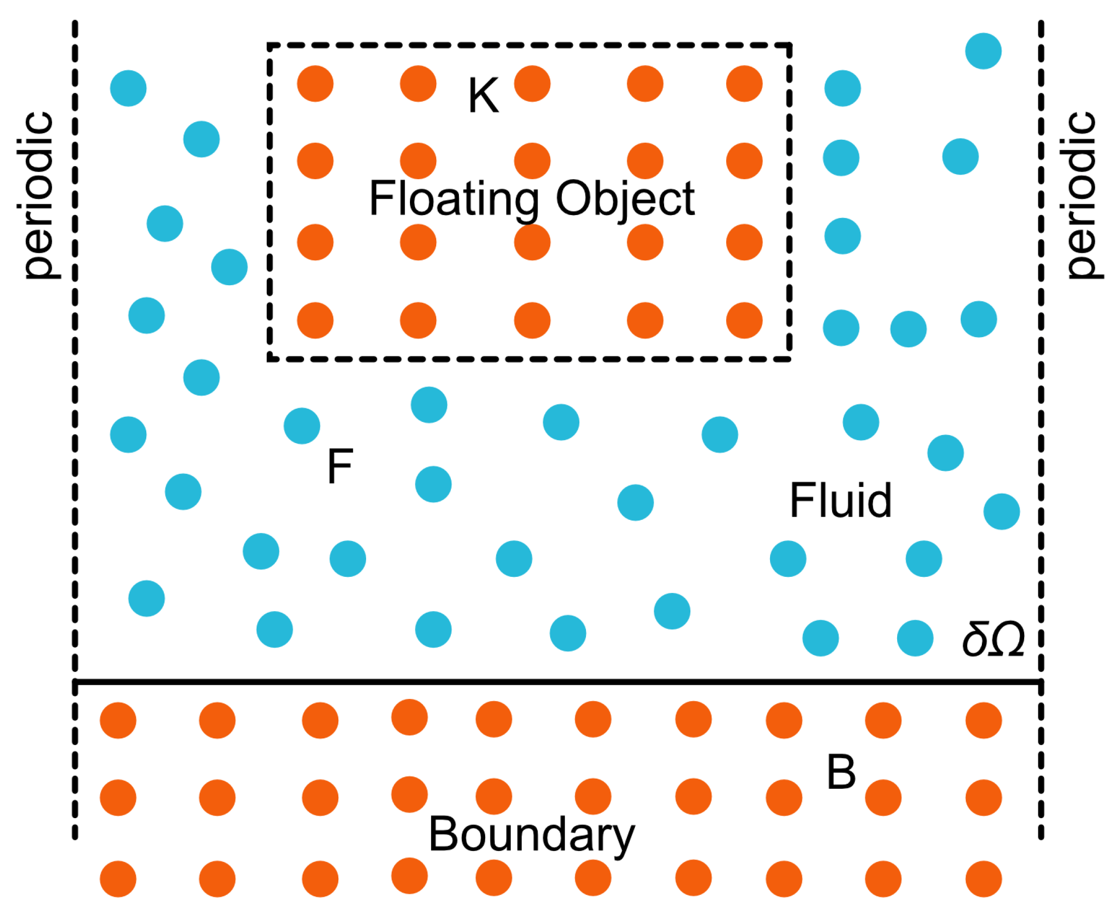
2.2.6. Boundary Conditions

Several boundary conditions are implemented in DualSPHysics. Solid boundary conditions are discretized by a set of boundary particles $a\in \mathbf{B}$ that differ from the fluid particles $\mathbf{F}$. Due to the Lagrangian nature of SPH, solid boundaries can also be moved straightforwardly according to user-defined motion.

Dynamic boundary conditions (DBC) are simply represented by fixed particles with density computed with the continuity equation and pressure obtained from the equation of state. Boundaries are easy to set up and computations are relatively stable and efficient, providing a robust option for complex geometries. Validations with dam-break flows and wave flumes have been published, and real engineering applications have been simulated successfully [65,66]. However, an unphysical gap between the fluid and these solid boundaries appears when fluid approaches to the boundary, decreasing the accuracy of pressures measured on the boundary. Therefore, a second approach is included now in DualSPHysics, where the density of solid particles is obtained from ghost positions within the fluid domain by linear extrapolation, described in [67]. With this second approach, the gap is avoided, and pressures of the boundary particles in still water converge to hydrostatic.

Dynamic boundary conditions The dynamic boundary condition (DBC) represents a solid wall using a collection of boundary particles $\mathbf{B}$, where the continuity equation is applied as described in [68]

$$\frac{d\rho }{dt}{|}_{a\in B}={\rho }_b\sum _{b\in F}\frac{m_b}{{\rho }_b}{\mathbf{v}}_{ab}·\nabla W,$$

(42)

while the position of these particles is updated following the equation

$$\frac{d\mathbf{v}}{dt}{|}_{\forall a\in B}={\mathbf{F}}^{\left(\mathrm{imposed}\right)}$$

(43)

where ${\mathbf{F}}^{\left(\mathrm{imposed}\right)}$ denotes the force exerted on moving boundary particles by the fluid. Such motion can be dictated by a predefined user function or by accelerations accumulated over time. The resultant increase in density from Equation (42) leads to an augmented pressure in the momentum equation for particle $a\in F$, creating a repulsive force between the fluid and boundary particles. This simplified boundary approach is especially suited for GPU implementation, allowing for code optimization through the use of vector lists. Further insights into this method can be found in Crespo et al. [68].

2.2.7. Particle Shifting Algorithm

The anisotropic distribution of particles introduces additional discretisation error through the zeroth- and higher-order kernel moments (i.e., the discrete version of Equation (3)). This is especially true in negligible or large dynamics [59] and violent flows where particles may not maintain an isotropic distribution. In DualSPHysics, the Fickian-based particle shifting algorithm of Lind et al. [69] is used to maintain a near isotropic particle distribution,

$$\delta {\mathbf{r}}_a{|}_{a\in F}=-D_s\nabla C_a,$$

(44)

where $\delta {\mathbf{r}}_a$ is the shifting distance, $\nabla C_a$ is the kernel gradient and $D_s$

$$D_s=A_{s}h\parallel {\mathbf{v}}_a\parallel \mathrm{\Delta }t,$$

(45)

where $A_s$ acts as a control parameter and $\parallel {\mathbf{v}}_a\parallel$ represents the magnitude of velocity for particle a [70]. A constraint based on the magnitude of particle velocity is applied to mitigate the risk of excessive displacement and the subsequent loss of data as particles transition across domain cells. The recommended range for $A_s$ is between one and six, with a preferred value of two as suggested by Skillen et al. [70]. Details for calculating $\nabla C_a$ can be found in [34].

2.3. DEM and DCDEM

Interactions between solids and fluids, as well as solid–solid interactions, are crucial issues in various engineering disciplines, including coastal, offshore, maritime, and river engineering. To address these interactions, DualSPHysics incorporates the Distributed Contact Discrete Element Method (DCDEM) into its Smoothed Particle Hydrodynamics (SPH) models for simulating fluid–solid interactions. This method, which calculates forces between a fluid and solid particle pair using SPH and models solid–solid interactions through DEM, is based on an explicit integration method and operates within the meshless framework of DualSPHysics. This innovative approach, initially introduced by Cummins and Cleary, enables the accurate representation of complex solid shapes through a particle-based method, with the particles subjected to a rigid body constraint. With the use of specific non-linear contact models, the system is capable of simulating a wide range of material behaviors using three primary parameters: Poisson ratio, Young’s modulus, and dynamic friction coefficient [71,72,73]. Despite its advantages, the model shares common limitations with general DEM approaches, such as potential stability issues due to its explicit nature, high computational demands or inaccuracies in simulating extended frictional contacts, and the risk of artificial effects in low-resolution simulations caused by the spherical particle shapes. Nevertheless, due to its simplicity and efficiency, it finds applications in evaluating hydrodynamic impacts on structures, assessing natural hazard risks, and designing both floating bodies and exposed structures.

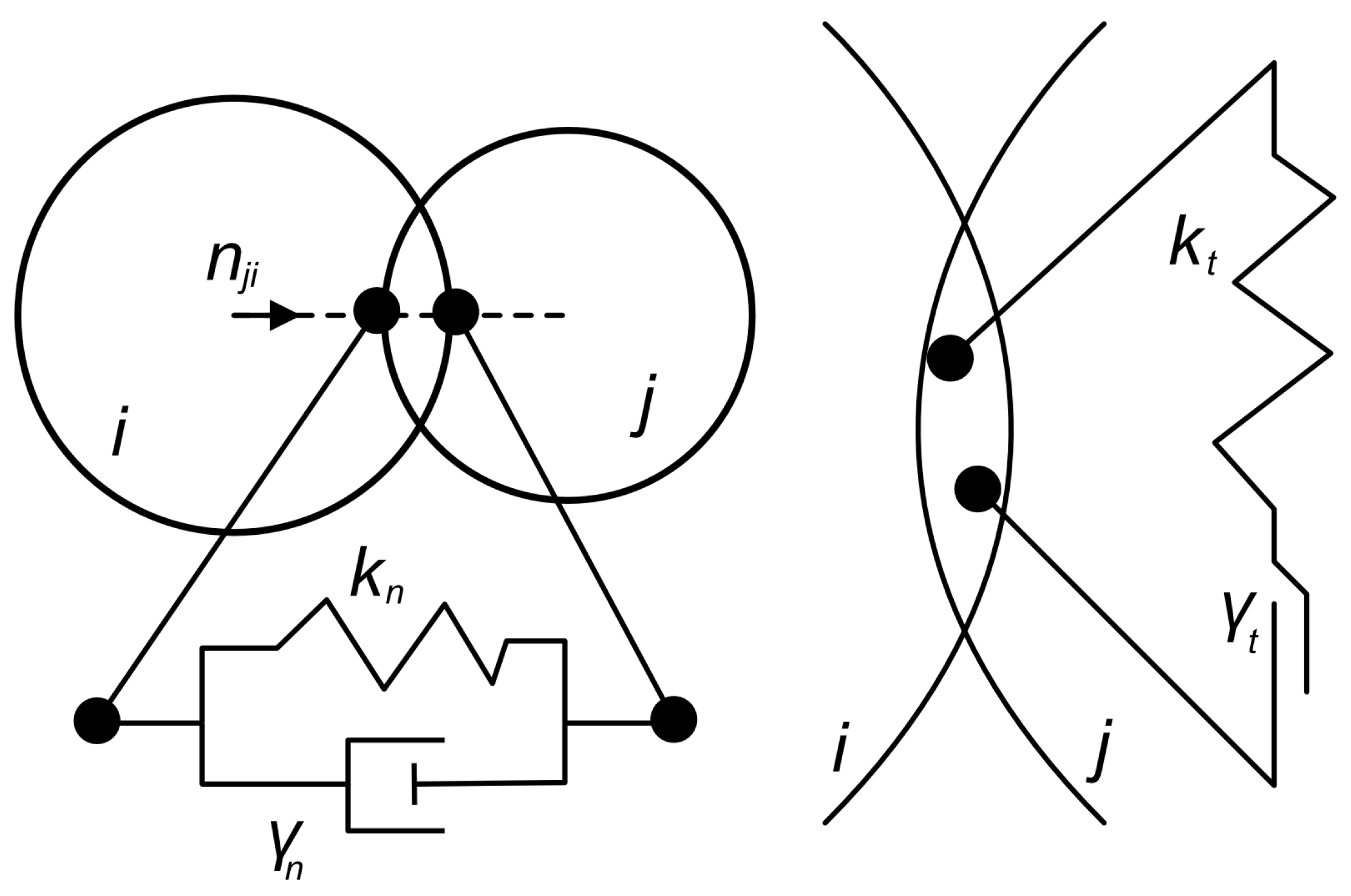
2.3.1. Method Formulation

In the framework of Smoothed Particle Hydrodynamics (SPH), the domain of the fluid is depicted through a constellation of nodal points. These points encapsulate essential physical parameters such as position, velocity, density, and pressure, approximated based on their spatial coordinates. Moving in sync with the fluid, adopting a Lagrangian viewpoint, the properties of these nodes are subject to change over time, influenced by their interaction with nearby nodes. The designation “Smoothed Particle Hydrodynamics” stems from the notion that these nodes essentially mirror the mass of a fluid segment, thereby being termed “particles”, and the smoothing over of their motion, ignoring individual rotational dynamics. This methodology is underpinned by the principles of integral interpolation theory [46]. An effective transition from a continuous integral representation to a discrete set of Lagrangian points is achieved through meticulous discretization:

$$A_i\approx \sum _j{A}_{j}W({\mathbf{r}}_{ij},h)V_j,$$

(46)

known as the summation approximation, is applied across all particles j, for which the distance $|{\mathbf{r}}_{ij}|=|{\mathbf{r}}_i-{\mathbf{r}}_j|$ does not exceed the smoothing length h. Here, $V_j$ represents the volume associated with particle j, $A_i$ denotes the variable being estimated at particle i, and W stands for the kernel, or weight, function. This approach indicates that achieving first-order consistency—wherein the kernel’s estimation precisely replicates a linear polynomial function—is not guaranteed. The limitation that arises due to the intrinsic errors linked to the discretized representation

$$\sum _j{V}_{j}W({\mathbf{r}}_{ij},h)\approx 1,$$

(47)

can become significant, especially near open boundaries or areas of discontinuity where the kernel W fails to maintain compact support. To address this, corrections such as Shepard’s method and Moving Least Squares (MLS) are often applied. Following the approach by Colagrossi and Landrini [74], spatial derivatives are determined through the gradient of the kernel. In this study, a Quintic kernel, as proposed by Wendland [44], is utilized:

$$W({\mathbf{r}}_{ij},h)={\alpha }_D{\left(1-\frac{q}{2}\right)}^4(2q+1),0\le q\le 2,$$

(48)

where $q=|{\mathbf{r}}_{ij}/h|$ and ${\alpha }_D=21/16\pi h^3$ for a 3D case.

2.3.2. Discretization of Rigid Body Equations and Contact Forces with DCDEM

In accordance with the original concept proposed by Koshizuka et al. [75], a rigid entity, denoted as I, is modeled utilizing a group of particles. These particles are arranged such that their relative positions do not alter, effectively allowing the volume of I to be represented by this particle ensemble. For ease of reference, this assembly is also labeled as I. These particles are subject to a unique set of equations distinct from those applied to conventional SPH particles. The dynamics of the rigid body are characterized by Newton’s laws, and the process of discretization is achieved by summing up the individual count

$$M_I\frac{d{\mathbf{V}}_I}{dt}=\sum _{k\in I}{m}_k\frac{d{\mathbf{v}}_k}{dt},$$

(49)

$$I_I\frac{d{\mathrm{\Omega }}_I}{dt}=\sum _{k\in I}{m}_k({\mathbf{r}}_k-\mathbf{R})\times \frac{d{\mathbf{v}}_k}{dt},$$

(50)

where the rigid body I is characterized by its mass $M_I$, velocity ${\mathbf{V}}_I$, inertia tensor ${\mathbf{I}}_I$, angular velocity ${\mathrm{\Omega }}_I$, and center of mass $\mathbf{R}$. These vectorial properties are recalculated at each time step. The force per unit mass acting on a particle k within the particle ensemble that constitutes I is represented by $m_k\frac{d{\mathbf{v}}_k}{dt}$, where $m_k$ signifies the mass of the particle k. This force integrates various effects including body forces such as gravity, fluid resistance, and the normal or frictional forces experienced during interactions with other solids. As such, the term $m_k\frac{d{\mathbf{v}}_k}{dt}$ can encompass a range of force types: interactions with fluid particles are governed by the fluid momentum equation, while interactions with solid particles are determined by additional derived forces. This cumulative approach to force calculation facilitates a seamless integration of solid and fluid dynamics.

Utilizing Equation (16) directly for the evaluation of local interactions between fluid and solid phases facilitates the incorporation of a viscous framework, thus providing a mechanism for viscous drag closure [76]. This model operates under the concept of Dynamic Boundary Conditions [68], and it adheres to the specifications outlined in Equations (49) and (50), without the need for any arbitrary, ad hoc adjustments. The dynamics are fully derived from the fundamental, particle-specific solutions of Equations (49) and (50). However, this formulation’s challenge lies in the propensity to overestimate density [77,78], a phenomenon linked to an entropy increase at the interface. This leads to an expansion in the spacing between fluid and solid particles due to the exerted pressure gradient force, thereby disrupting the accuracy of viscous force calculations at that interface [74]. The addition of the $\delta$-SPH diffusive term within Equation (15) is suggested as a remedy, enabling an ostensibly precise density estimation at the interface [76].

In the scenario where two particles, either part of a boundary or a rigid body, interact, they exhibit dynamics governed by the Discrete Element Method (DEM). The resultant contact force ${\mathbf{F}}_i^{\mathrm{T}}$ on particle i, due to a collision with particle j, is analyzed into ${\mathbf{F}}_n$ and ${\mathbf{F}}_t$, which correspond to the normal and tangential force components, respectively. These components are further subdivided into a repulsion force ${\mathbf{F}}^r$, generated by the material’s deformation, and a damping force ${\mathbf{F}}^d$, aimed at energy dissipation throughout the deformation process. The mechanics of DEM interactions between two particles are visually demonstrated in Figure 3.

The normal forces are given by a modified, non-linear, Hertzian model [72,79]

$${\mathbf{F}}_{n,ij}={\mathbf{F}}_n^r+{\mathbf{F}}_n^d=k_{n,ij}{\delta }_{ij}^{3/2}{\mathbf{e}}_{ij}-{\gamma }_{n,ij}{\delta }_{ij}^{1/4}{\dot{\delta }}_{ij}{\mathbf{e}}_{ij},$$

(51)

where the stiffness constant for the interacting pair $ij$ is $k_{n,ij}$, and the particle overlap ${\delta }_{ij}=max(0,(d_i+d_j)/2-|{\mathbf{r}}_{ij}\left|\right)$ approximates material deformation. The unit vector between the centers of mass of the particles is denoted as ${\mathbf{e}}_{ij}$, with the rate of normal deformation given by ${\dot{\delta }}_{ij}={\mathbf{v}}_{ij}·{\mathbf{e}}_{ij}$, and the damping constant is ${\gamma }_{n,ij}$. This non-linear formulation helps mitigate some of the limitations inherent in using constant restitution coefficients and fixed contact durations for particle pairs, effectively capturing more physically representative behaviors for a broad spectrum of contacts [80]. The stiffness and damping constants are given by

$$k_{n,ij}=-\frac{4}{3}{E}^{*}\sqrt{R^{*}};{\gamma }_{n,ij}=C_n\sqrt{6M^{*}{E}^{*}\sqrt{R^{*}}},$$

(52)

with $C_n$ of the order of ${10}^{-5}$ [81]. The other parameters are given by

$$\frac{1}{E^{*}}=\frac{1-{\nu }_I^2}{E_I}+\frac{1-{\nu }_J^2}{E_J};R^{*}=\frac{r_i{r}_j}{r_i+r_j};$$

(53)

$$M^{*}=\frac{m_I{m}_J}{m_I+m_J},$$

(54)

where E is the Young modulus, $\nu$ is the Poisson ratio, and m is the mass of the body.

For tangential interactions among particles, friction is depicted through a linear dashpot model, limited by the Coulomb friction law’s maximum force, which is defined by the kinetic friction coefficient ${\mu }_f$. This linear methodology represents a compromise between the fidelity of the model and its computational feasibility. While more elaborate models yield better performance for specific situations, such as rolling friction, their effectiveness is generally limited in broad application scenarios. A sigmoidal function modifies the Coulomb law to ensure continuity at the origin concerning tangential velocity, smoothing the transition and enhancing the model’s realism [82]:

$${\mathbf{F}}_{t,ij}=min({\mu }_{f,IJ}{\mathbf{F}}_{n,ij}tanh\left(8{\dot{\delta }}_{ij}^t\right){\mathbf{e}}_{ij}^t·({\mathbf{F}}_t^r+{\mathbf{F}}_t^d),$$

(55)

where

$${\mathbf{F}}_t^r+{\mathbf{F}}_t^d=k_{t,ij}{\delta }_{ij}^t{\mathbf{e}}_{ij}^t-{\gamma }_{t,ij}{\dot{\delta }}_{ij}^t{\mathbf{e}}_{ij}^t.$$

(56)

The model employs a penalty method to replicate the mechanisms of static and dynamic friction. Rather than allowing the body to adhere statically at the point of contact, it is governed by a spring-damper mechanism. With the premise that the time scales for normal and tangential contacts are identical, ref. [83] established that the tangential stiffness could be calculated as $k_t=\frac{2}{7}{k}_n$. To adequately reflect the time scale of rigid contacts and maintain the system within its stability region, an additional component is required to be incorporated into the dynamic equation as indicated by [81]:

$$\mathrm{\Delta }{t}_{\mathrm{DEM}}=\underset{i}{min}\left(\frac{\pi }{50}\sqrt{\frac{k_{n,ij}}{m_{IJ}}}\right).$$

(57)

This class of DEM model is refereed to as a ‘soft sphere’ approach since it depends on the particle overlap to deform the spring-damper system. This formulation provides a force estimate particle-wise which, coupled with the rigid body idea, allows the generalization of the geometry by not requiring information on normal directions or other forms of topology, solving for arbitrarily complex geometries by resolving the local interactions.

3. Materials and Methods

This study endeavors to apply the Discrete Element Method (DEM) for the simulation of the grinding media and Smoothed Particle Hydrodynamics (SPH) for the simulation of the slurry. Experiments are performed with the use of copper ore. The experiments consist of 3 stages: calibration of the behavior of the balls; calibration of the dry milling; and calibration of the wet milling. Experiments are recorded with the high-speed camera and then processed with computer vision methods. The simulations are performed with the open-source DualSPHysics simulation frameworks, which consist of a set of C++ and CUDA code, enabling fast simulation using GPU.

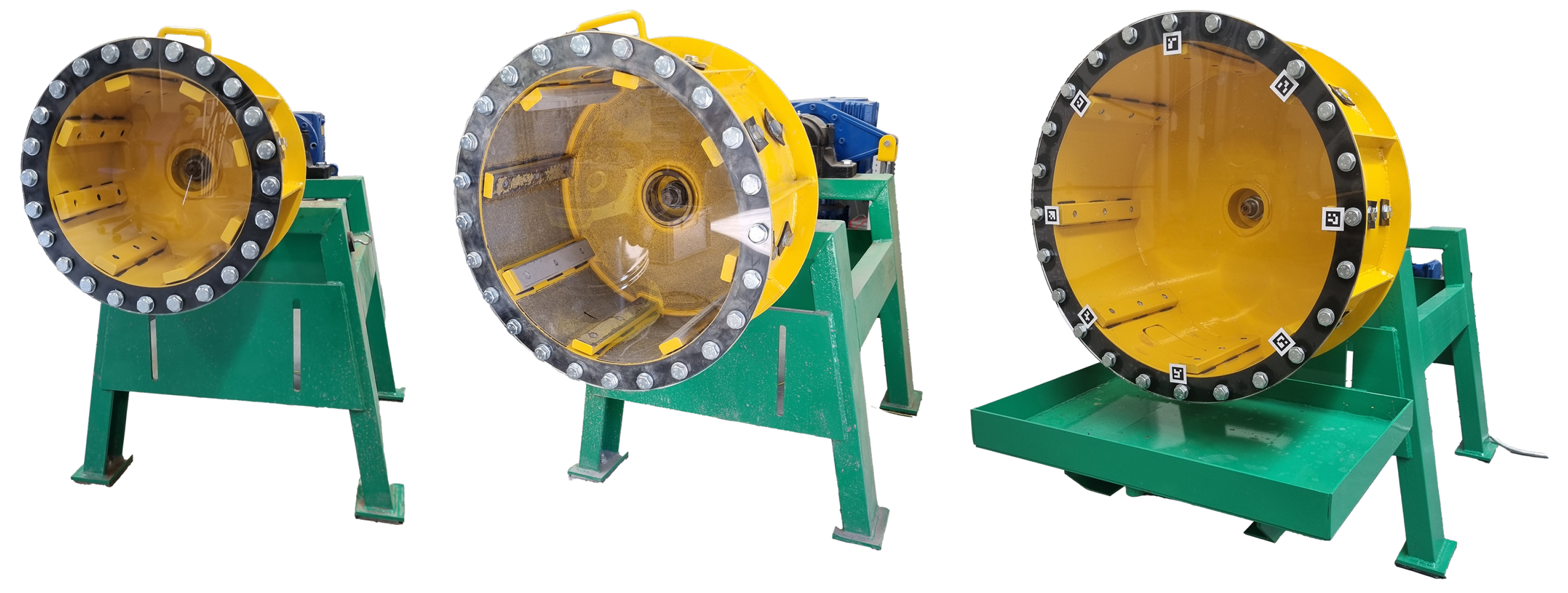
3.1. Experimental Setup

The experimental test stand consists of the laboratory scale ball mill with exchangeable drums (Figure 4). In the experiments, 3 different mill drum diameters are used, with external diameters of 300, 400, and 500 mm. The internal diameter of each drum is 8 mm smaller. The laboratory mill is equipped with a transparent wall, allowing for the real-time recording of the milling process. This setup is crucial for the subsequent computer vision analysis. The recordings are made with a speed of 300 fps with a Phantom v2512 camera.

3.2. Copper Ore and Its Slurry Properties

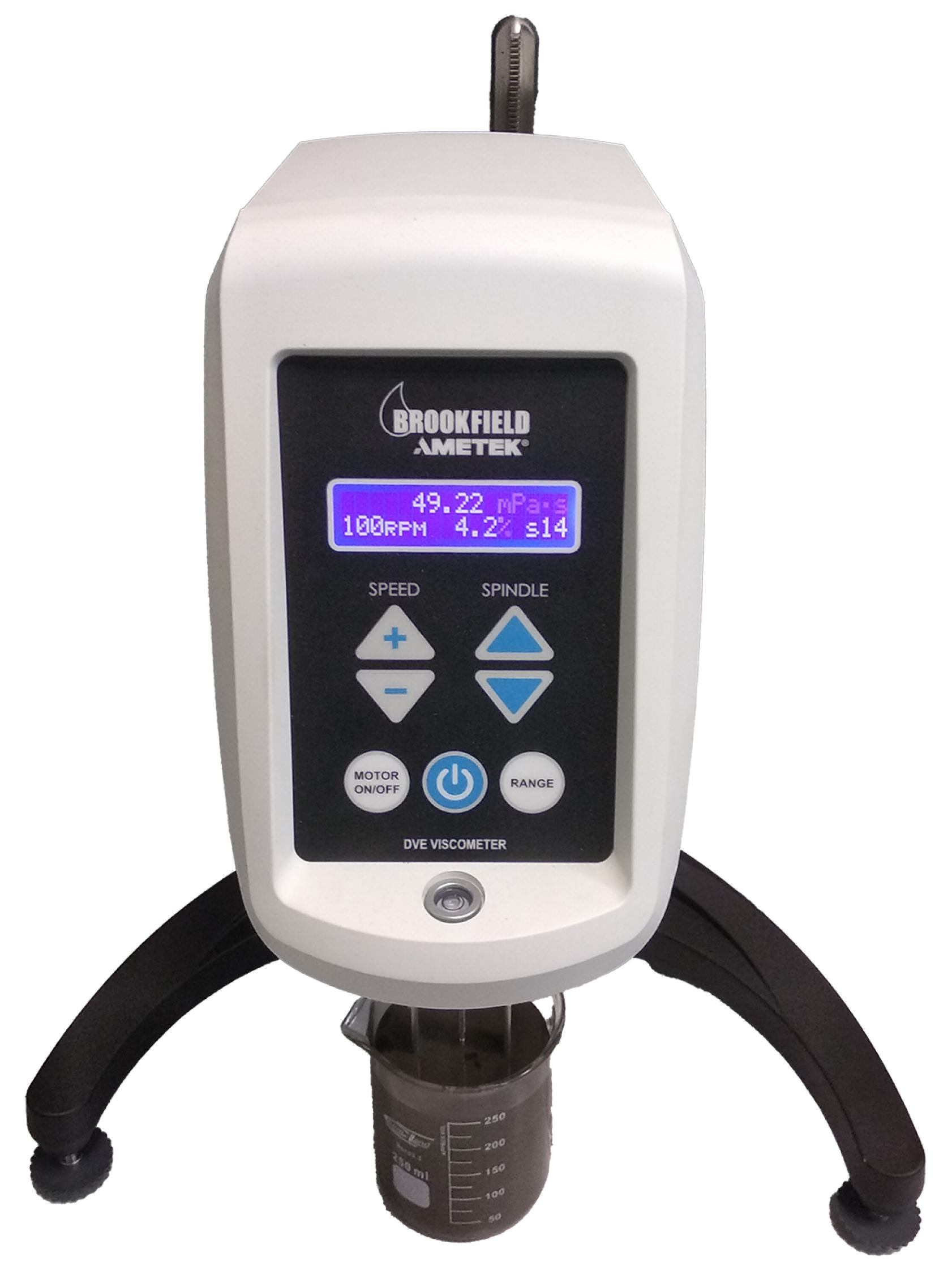
The copper ore tested exhibits a density of $2194.93\pm 98.51{\mathrm{kg}/\mathrm{m}}^3$, with the dominant grain size ($d_{80}$) being approximately 1 mm. This section delves into the critical aspect of viscosity related to the ore and its slurry, presenting it in a manner that aims to be accessible to a diverse audience while retaining the precision expected in scientific discourse.

3.3. Viscosity

Absolute Viscosity: This is measured in poiseuille (Pl), which is equivalent to $\mathrm{kg}{\mathrm{m}}^{-1}{\mathrm{s}}^{-1}$ or Newton-second per square meter ($\mathrm{N}\mathrm{s}{\mathrm{m}}^{-2}$). It represents the internal friction within a fluid [84].

Kinematic Viscosity: Unlike absolute viscosity, kinematic viscosity does not have a named SI unit and is expressed in square meters per second (${\mathrm{m}}^2{\mathrm{s}}^{-1}$). It is obtained by dividing the absolute viscosity by the fluid’s density, $\nu =\frac{\mu }{\rho }$, where ${\nu }_k$ is the kinematic viscosity, $\mu$ is the absolute viscosity, and $\rho$ is the density of the fluid [84]. It is noteworthy that while the viscosity of gases increases with temperature, the opposite is true for liquids [84].

3.4. Application to Copper Ore Slurry

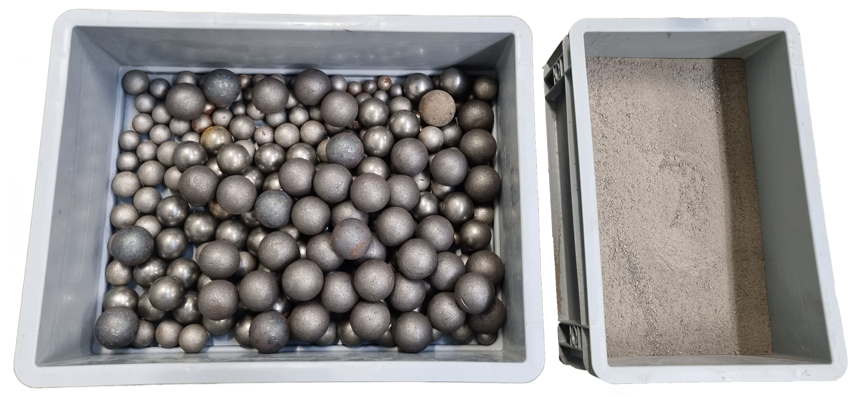
The slurry used for model calibration presented a density of $1400{\mathrm{kg}/\mathrm{m}}^3$. The density was approximated by mixing ore and water based on their known densities, aiming for a reproducible method suitable for industrial scaling, with adjustments made to acknowledge that achieving an exact density is challenging but the target density is closely approximated through direct mixing in specific proportions. Experiments measured the slurry’s viscosity across different densities and milling times, utilizing a viscometer AMETEK Brookfield (Figure 5).

A Random Forest Regressor model was developed to predict the absolute viscosity, ${\nu }_a$, in Pascal-seconds ($Pa·s$), considering milling time and density as variables. The model, demonstrating an R-squared value of 0.8402, indicates a good fit to the data and reliable prediction capabilities.

For a specific test scenario with a slurry density of $1400{\mathrm{kg}/\mathrm{m}}^3$ and a milling time of 15 min, the model predicted an absolute viscosity of approximately 0.01134 $\mathrm{P}\mathrm{a}·\mathrm{s}$. This provided a realistic prediction of resistance to flow within the slurry.

The kinematic viscosity $\nu$ for the copper ore slurry was then calculated by dividing the absolute viscosity by the slurry’s density. Given a predicted absolute viscosity of 0.01134 $\mathrm{P}\mathrm{a}·\mathrm{s}$ and a slurry density of $1400{\mathrm{kg}/\mathrm{m}}^3$, the kinematic viscosity of the copper ore slurry was calculated as:

$$\nu =\frac{0.01134}{1400}\approx 8.10\times {10}^{-6}{\mathrm{m}}^2/\mathrm{s}$$

This positive value of kinematic viscosity reflects the material’s resistance to flow and is indicative of the slurry’s physical behavior under the given conditions.

3.5. Grinding Media

The grinding media utilized in our experimental setup consisted of steel balls with a makeup diameter of 35 mm. These balls were selected for their uniformity in size and a precisely measured density of $7800.92\pm 55.41{\mathrm{kg}/\mathrm{m}}^3$. To ensure a comprehensive understanding of different load behaviors and to enhance the model’s adaptability to various grinding media size distributions, we employed a range of ball sizes from 15 mm to 35 mm, with each size differing by 5 mm. The selection of ball sizes was specifically tailored to the drum size utilized in the experiments: for a 500 mm drum, ball sizes ranged from 25 to 35 mm; for a 400 mm drum, from 20 to 35 mm; and for a 300 mm drum, from 15 to 35 mm.

The distribution of steel ball sizes was determined based on the Bond equilibrium state as described by the equation [85,86]:

$$y={\left(\frac{x}{B}\right)}^{3.8}$$

where we have the following:

• y represents the percentage of the total equilibrium charge that passes a given size x (mm);
• B denotes the makeup/recharge size of the balls (mm).

3.6. Operational Parameters

The milling operations were conducted with a filling degree of 0.5, wherein 60% of the filled mill’s volume was occupied by steel balls, translating to 30% of the mill’s total volume given the dynamic nature of milling and the fact that in practice, only 50% of the mill’s internal volume is effectively utilized for the balls and the material being milled. The remainder of the volume was considered void space between the balls for calibration purposes in the first step. In dry milling configurations, this void space was filled with ore, while for wet milling, a mixture of water and ore was utilized to achieve the desired slurry density. The selection of the quantity of balls of specific sizes was determined based on the equations detailed in the paper [85]. Figure 6 shows an example of the mill filling in the form of material and grinding media-balls.

The rotational velocity of the mill was set to 30% of the critical speed, a value calculated specifically for each experiment to accurately represent the dynamics of the load within the mill drum. It is crucial to note that while the speed was maintained at 30% of the critical speed for all tests, the nominal speed in RPM varied according to the mill diameter: 24.8, 21.1, and 18.7 RPM for diameters of 300, 400, and 500 mm, respectively. This approach ensured that the desired material behavior was achieved without the material being excessively lifted or failing to descend the "slope" created by the grinding media. Achieving consistent behavior across different mill sizes and speed settings, akin to the material’s real-world response at 30% of the critical speed, served as an additional layer of validation. The critical speed marks the threshold at which the centrifugal forces acting on the balls equal the gravitational forces, ensuring that the grinding media are carried around in a fixed movement pattern without dropping, a condition essential for efficient grinding.

The critical speed ($N_c$) in revolutions per minute (RPM) was derived from the balance of gravitational and centrifugal forces, and is given by the formula [87]:

$$N_c=\frac{1}{2\pi }\sqrt{\frac{g}{R-r}}\times 60$$

where we have the following:

• g is the acceleration due to gravity ($9.81{\mathrm{m}/\mathrm{s}}^2$);
• R is the radius of the mill (in meters);
• r is the radius of the balls (in meters).

This formula is derived from setting the centrifugal force equal to the gravitational force acting on a ball within the mill. This equilibrium point is crucial for determining the optimal operating speed of the mill to ensure the grinding media are the most effective. The value was calculated for the average ball diameter in the load for each experiment.

For all experiments, the mill drums were equipped with eight 5 mm lifters evenly spaced along the interior surface of the drum. This setup was designed to ensure uniform distribution of the grinding media and the material being milled, optimizing the milling efficiency and reproducibility of the results.

The grain composition of the ground ore was standardized, and all experiments were conducted on ore with a grain size below 2 mm, with a d80 grain size of 0.876 mm.

3.7. Computer Vision Analysis

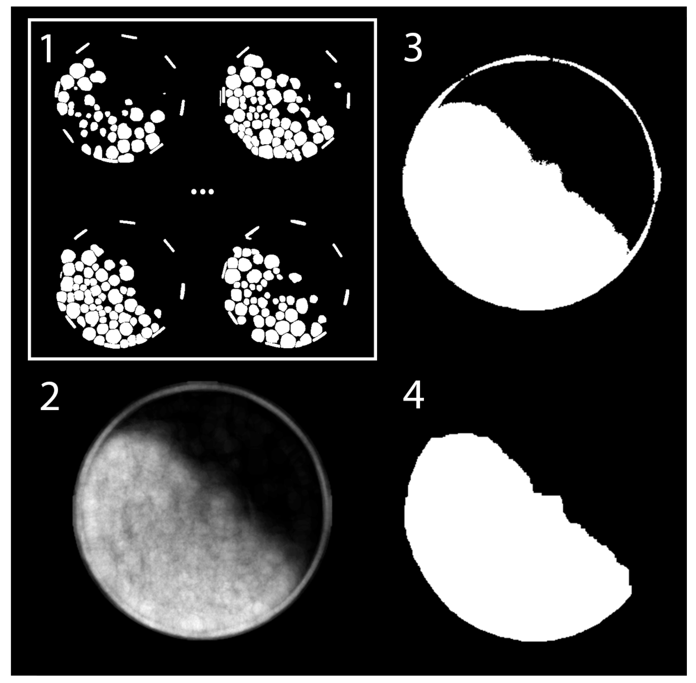
This section details the methodologies applied in analyzing the dynamic angle of repose and the slurry surface position in milling operations through computer vision. The analysis encompasses three scenarios: operations with balls only, dry milling, and wet milling. Each scenario incorporates a blend of image processing techniques and machine learning models to gain insights into the efficiency of the milling process.

Prior to analysis, all scenarios necessitate image pre-processing, which involves loading video, sampling frames at regular intervals. These frames undergo several processing steps using the OpenCV Python library, including mill outline detection via the Hough Circle Transform (Figure 7), centering frames, resizing to match actual dimensions, and applying a mask to obscure everything outside the mill (Figure 8), focusing only on the drum’s internal part.

For each recording, a set of 100 frames with equal time step between them is used.

3.7.1. Only Balls

This analysis utilizes the Segment Anything Model (SAM) developed by Meta, a pre-trained AI model specializing in segmenting images and applying masks [88]. The methodology unfolds as follows:

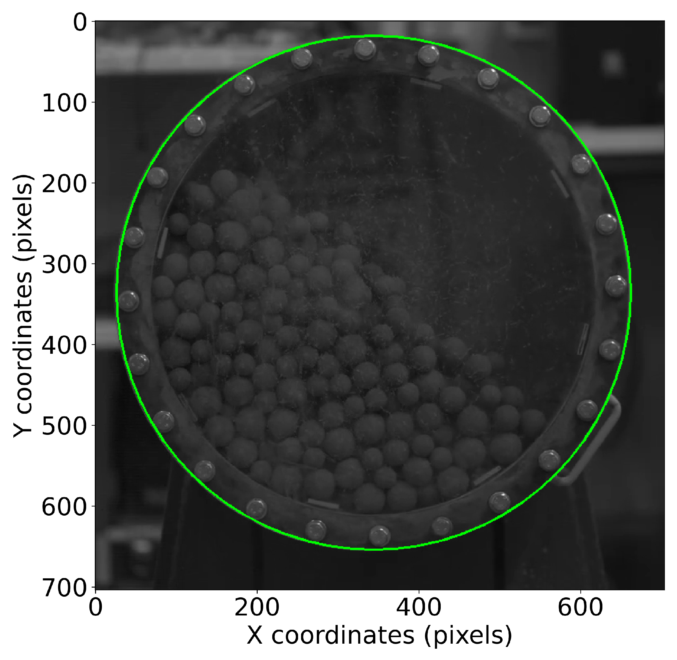
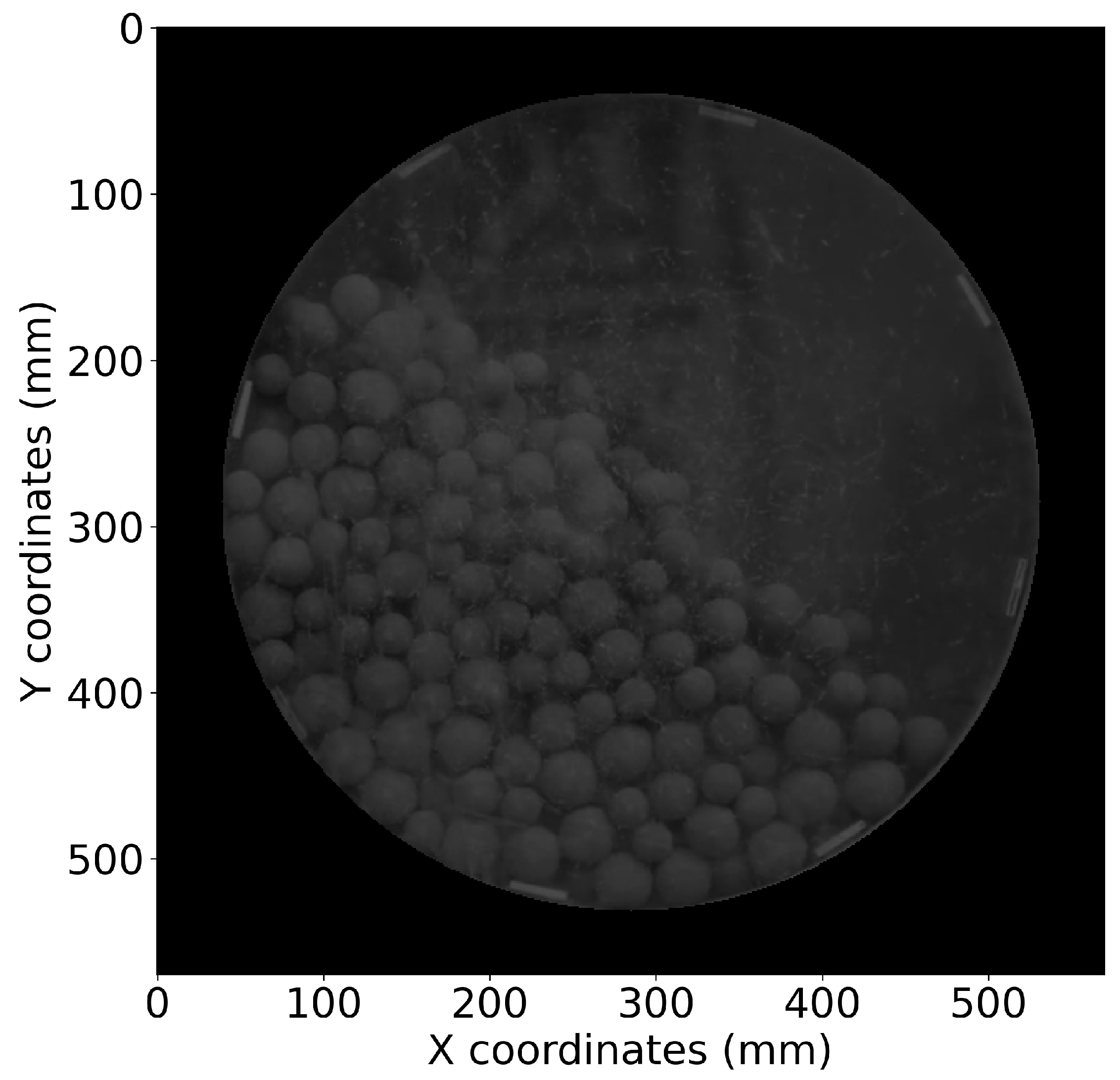
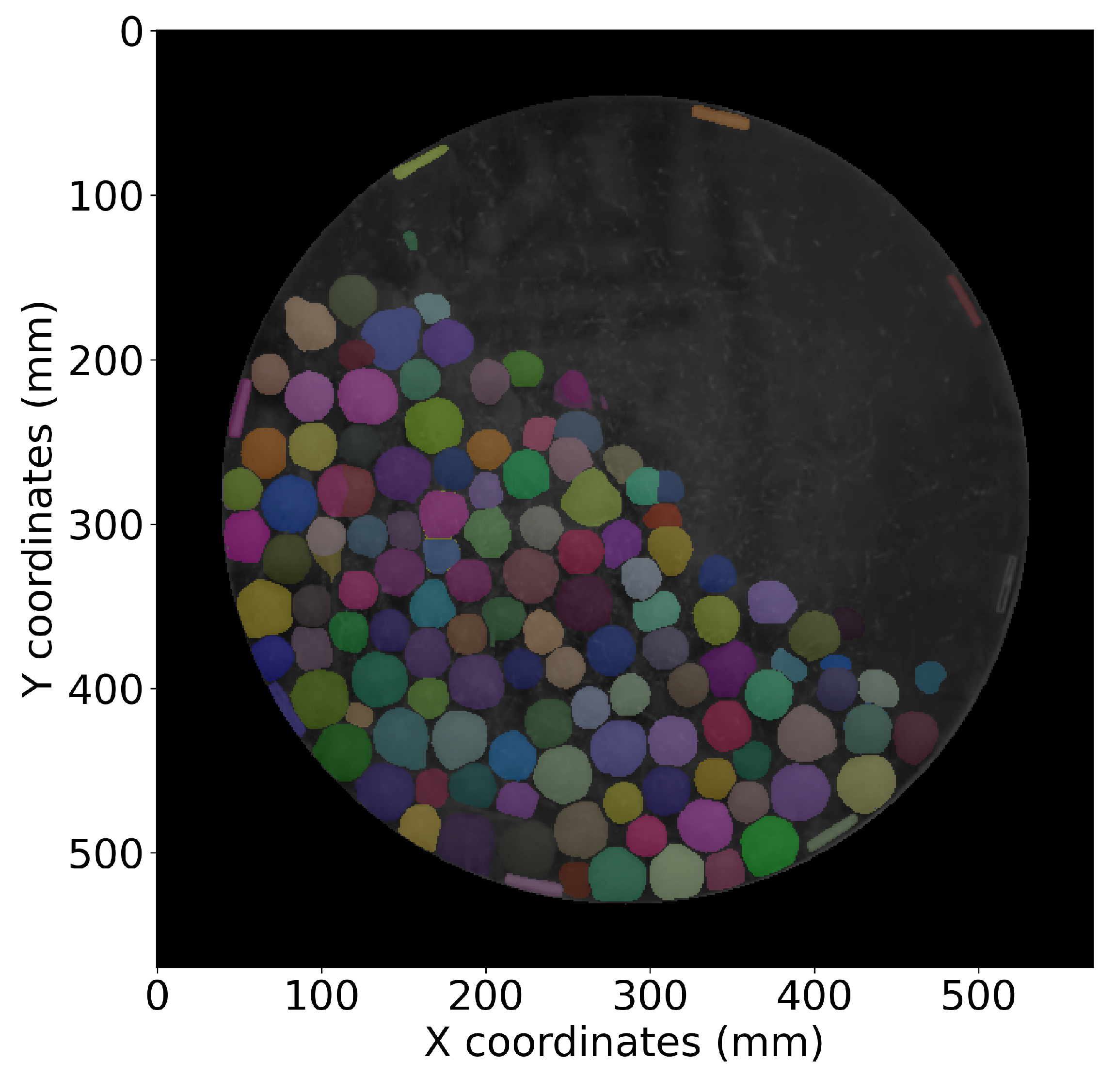
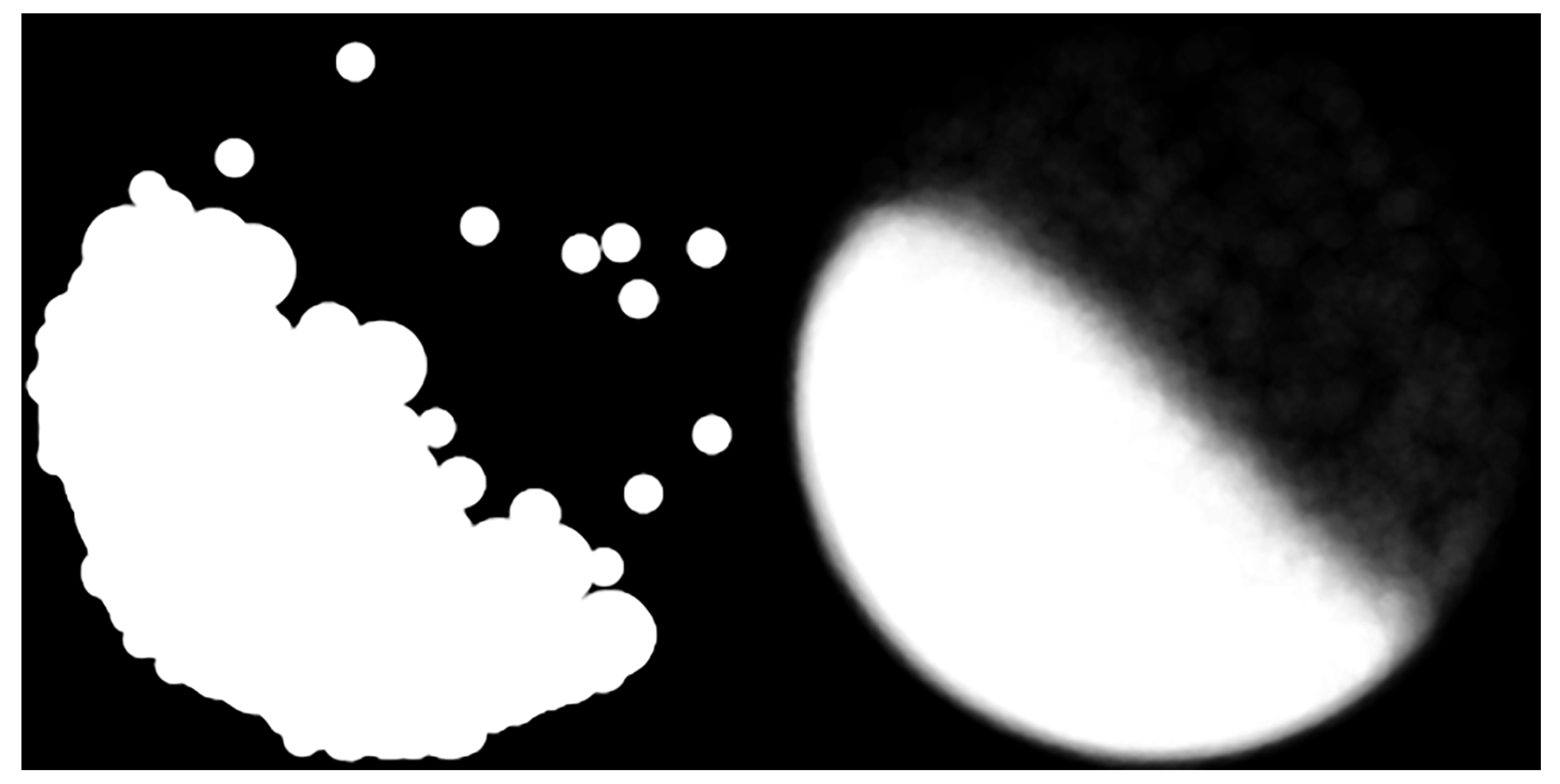
• Ball Detection and Mask Generation: Utilize the SamAutomaticMaskGenerator from the SAM library to produce masks for the detected balls (Figure 9).
• Heatmap Generation and Processing: Generate a heatmap from accumulated binary masks to pinpoint regions with frequent ball presence. Then, to the heatmap, thresholding is applied, and finally the image is smoothed with the smoothing kernel (Figure 10).
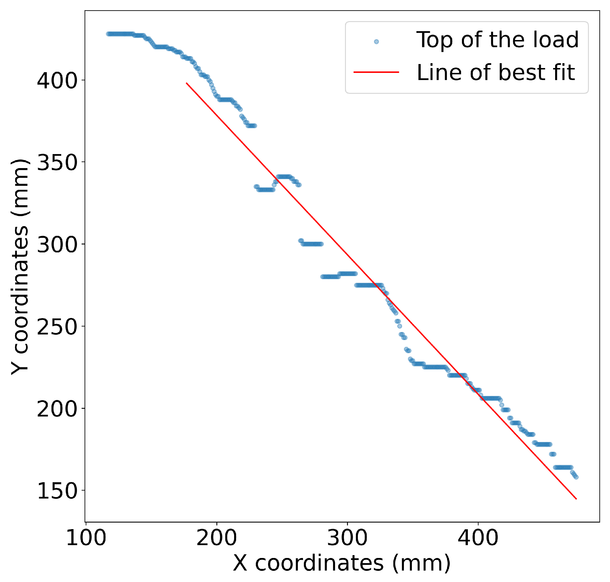
• Top Edge Detection and Angle Calculation: Then processed image is used to detect highest position of the white pixel, and a set of y coordinates for each x coordinate is extracted from the image. Dynamic angle of repose is obtained through linear regression, employing the scikit-learn Python library. Linear regression is performed on the points starting from the 60 mm to the right from the highest detected point, so the most linear part of the repose surface would be analyzed (Figure 11).
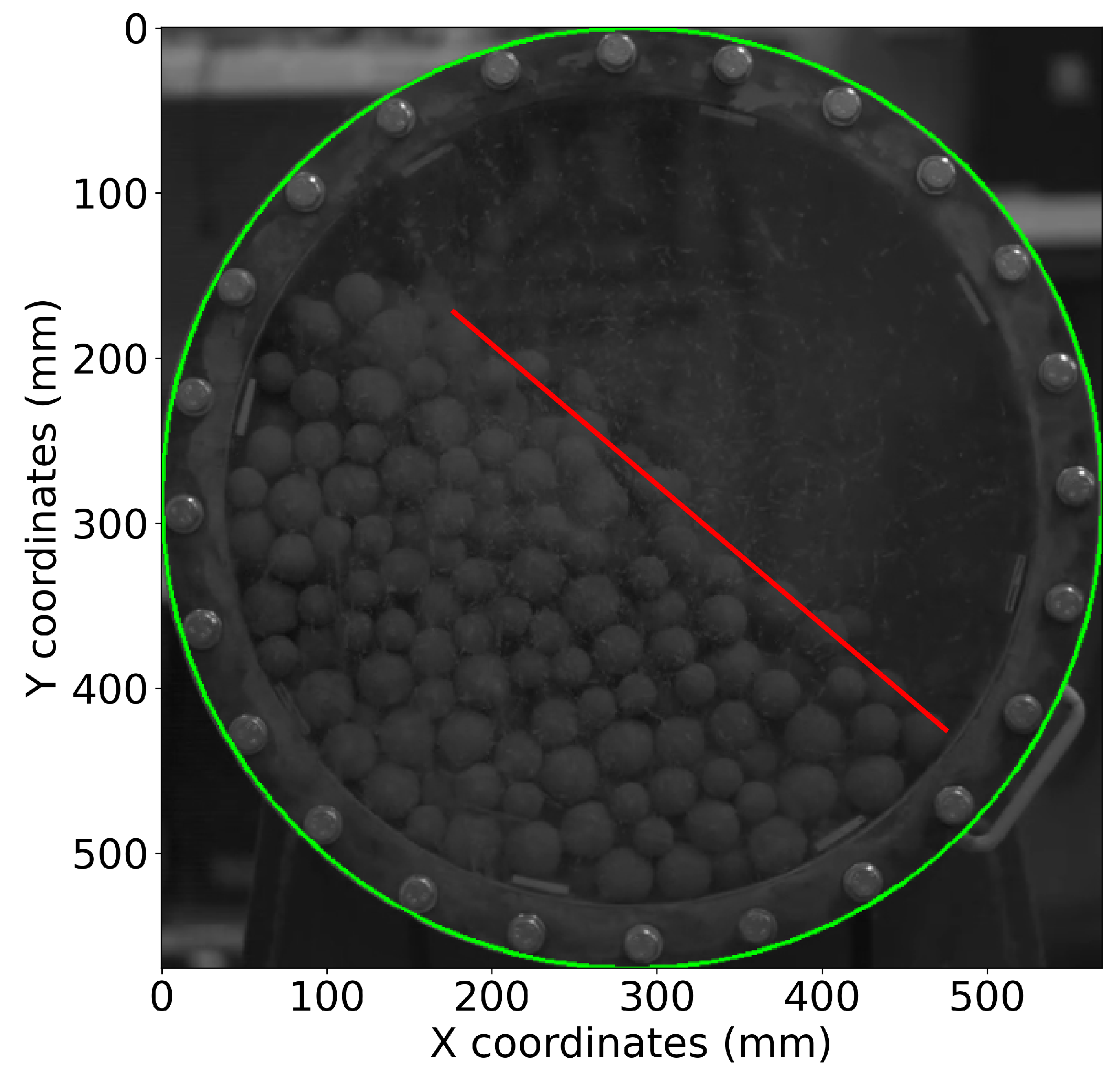
• Visualization and Output: Display the line obtained from the calculated dynamic angle of repose for debugging and threshold adjustment purposes (Figure 12).

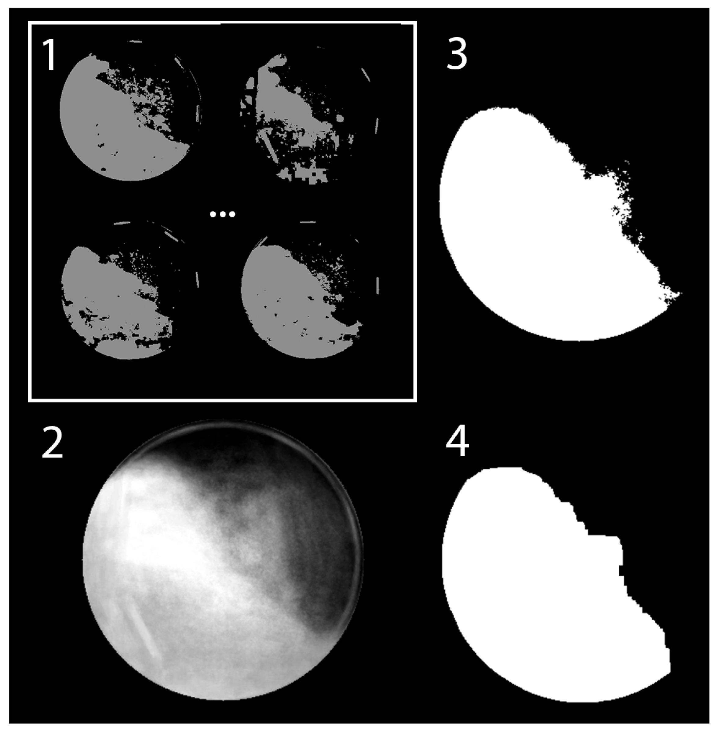
3.7.2. Dry Milling

This approach differs in the initial detection and isolation of the mill load area and the creation of binary images, reflecting the complexity of processing mixed loads (Figure 13). The difference in this approach is presented in the way that here, thresholding is directly used on the preprocessed image to generate binary images for further analysis.

3.7.3. Wet Milling

Wet milling operations present unique challenges, making computer vision models unsuitable for extracting the mill load area. Consequently, an interactive GUI interface was developed to address these obstacles. The load, barely visible through the slurry-covered transparent wall, necessitates a procedure combining manual point selection with curve fitting techniques. In this scenario, the top surface of the liquid is analyzed rather than measuring the angle of repose.

Because of the obstacles described before, only the recording of the mill with the biggest drum was suitable for the calibration of the wet milling. The medium and small size drums did not provided enough valuable data to process them the same way.

During milling experiments, the observation was made that when ball load is under the slurry, the whole transparent wall area is equally covered with the slurry and nothing is visible, but when balls appear over the slurry surface, they start to wipe off parts of the slurry from the transparent wall. This phenomenon was manually caught to measure the approximate location of the slurry surface.

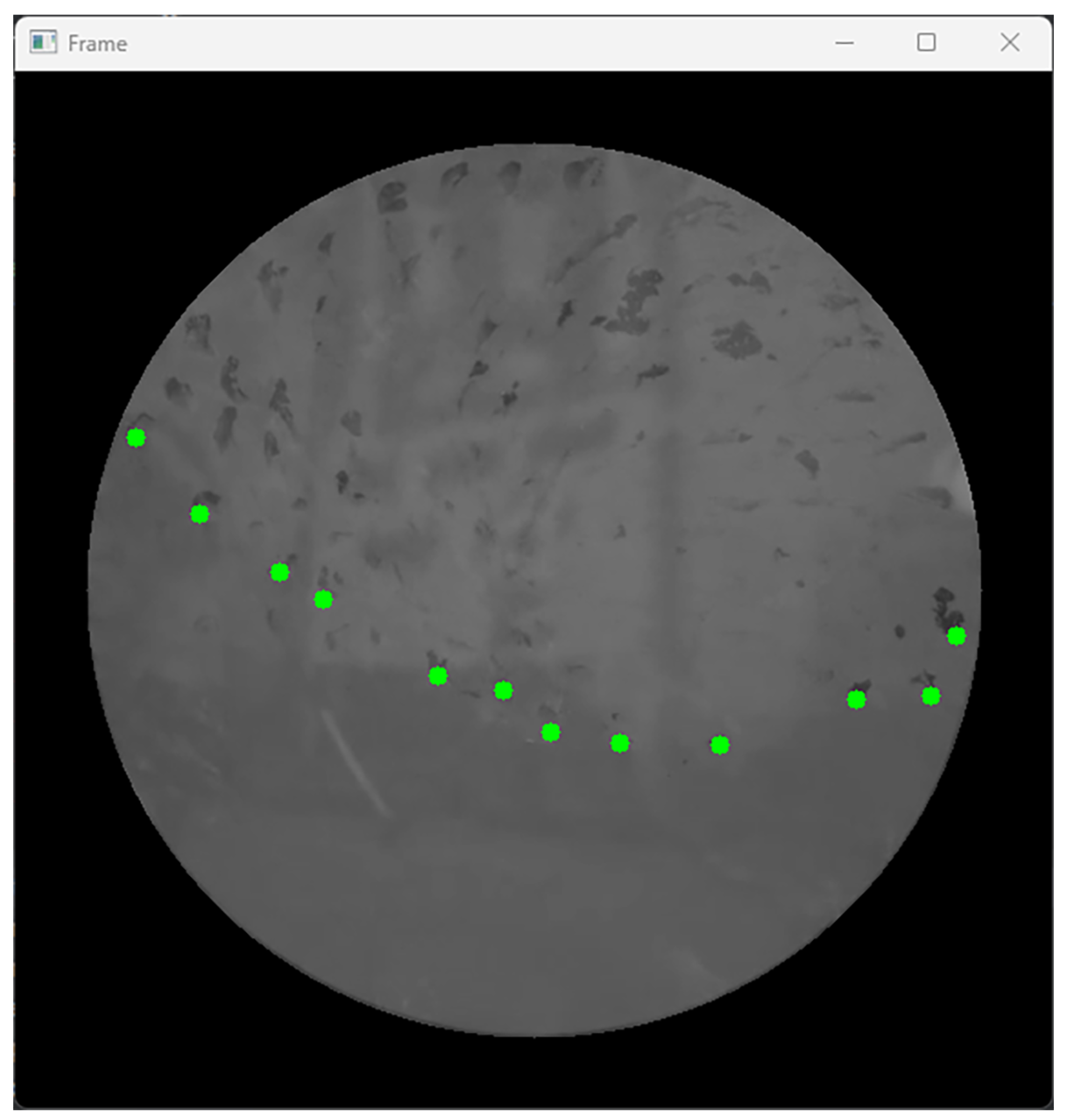
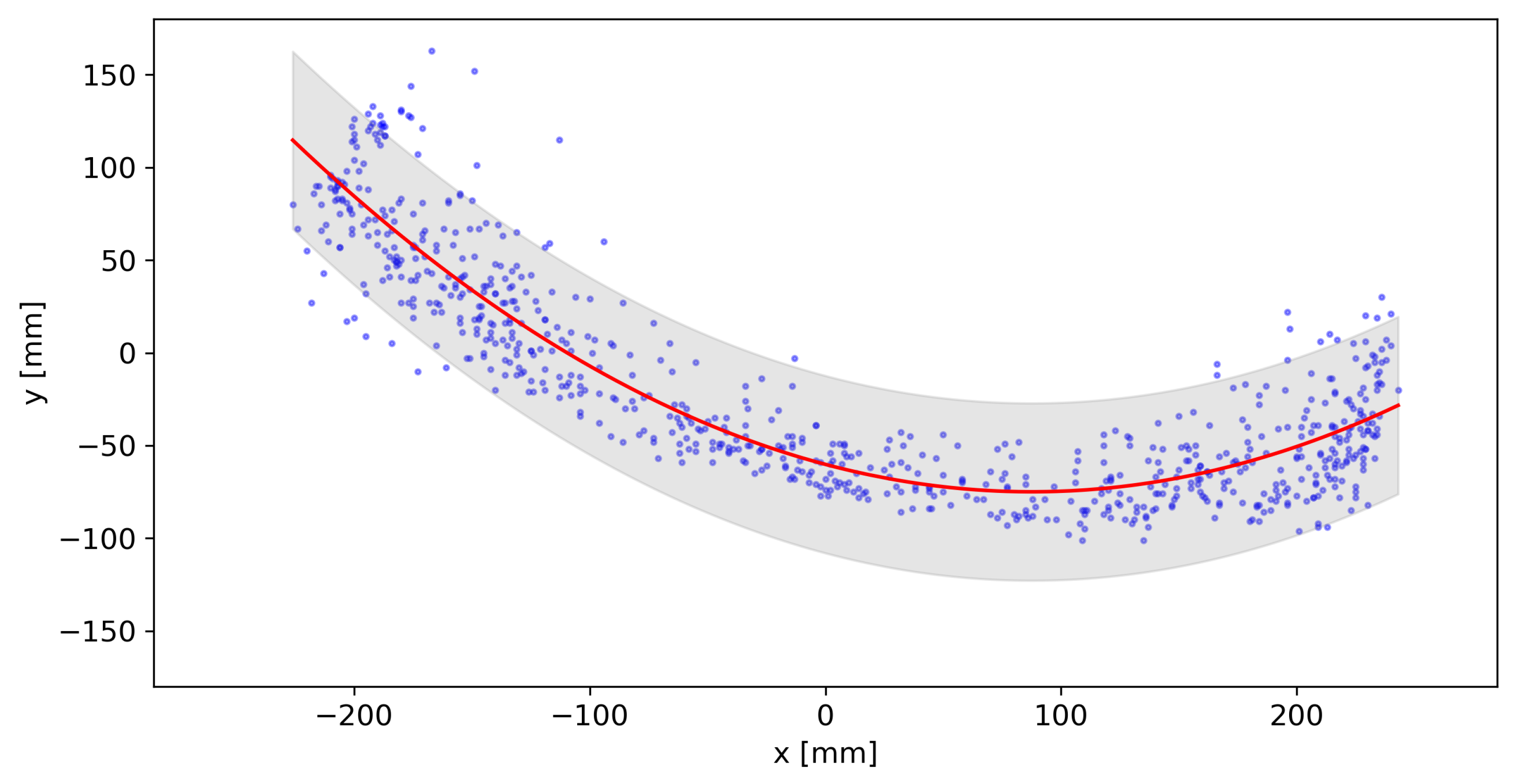
• Manual Point Selection: Conduct a manual analysis using a custom interface to select points delineating the wet load’s boundary (Figure 14).
• Data Preparation and Correction: Prepare and correct the selected points for the analysis coordinate system, emphasizing accuracy verification.
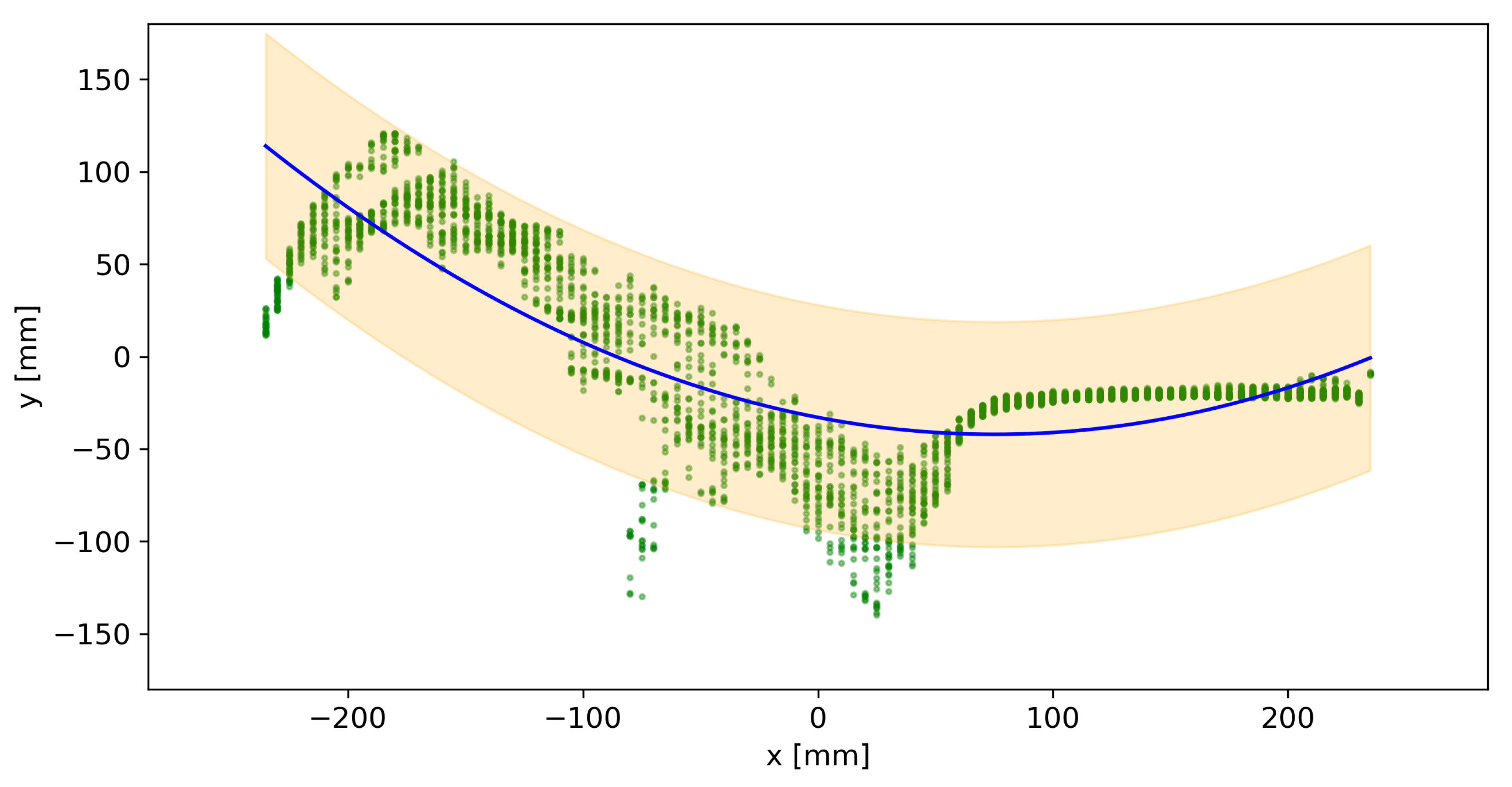
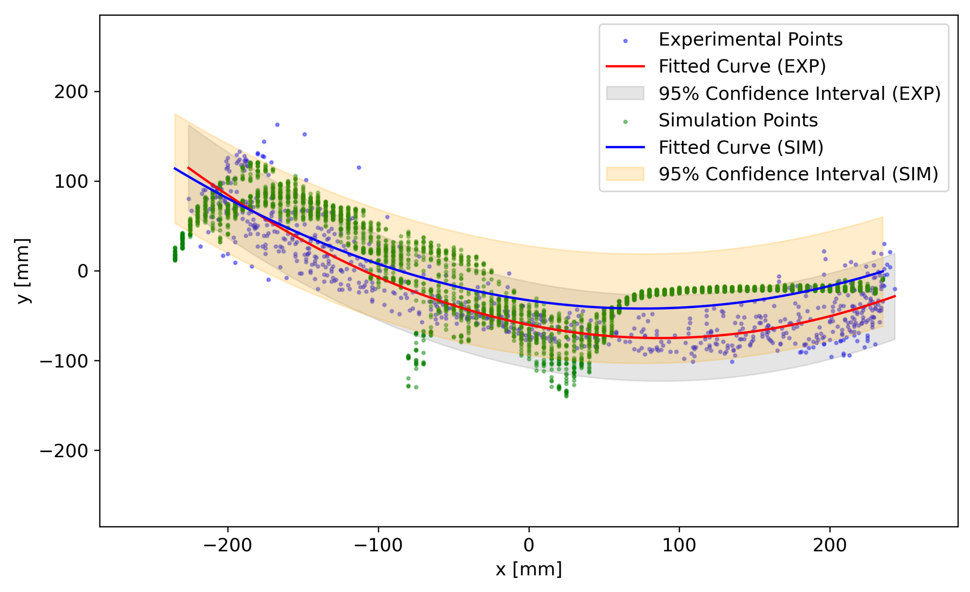
• Curve Fitting and Analysis: Perform curve fitting to model the load’s boundary, calculate the fit’s parameters, and evaluate the fit’s uncertainty.
• Visualization and Interpretation: Display the fitted curve alongside the original data points and confidence interval bounds.

This methodology distinctively blends manual interaction and statistical modeling to analyze wet milling dynamics, utilizing tools such as OpenCV, matplotlib, pandas, and scipy for thorough data management and analysis.

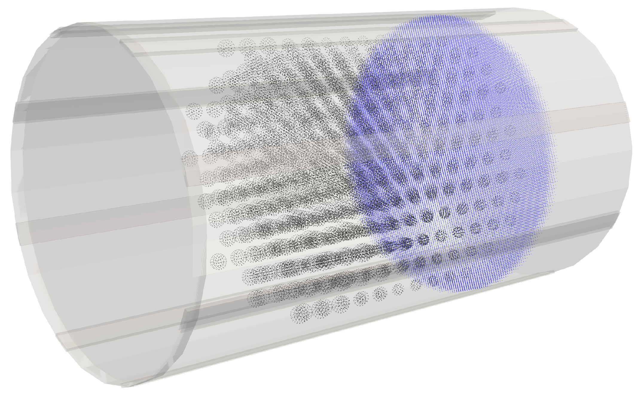
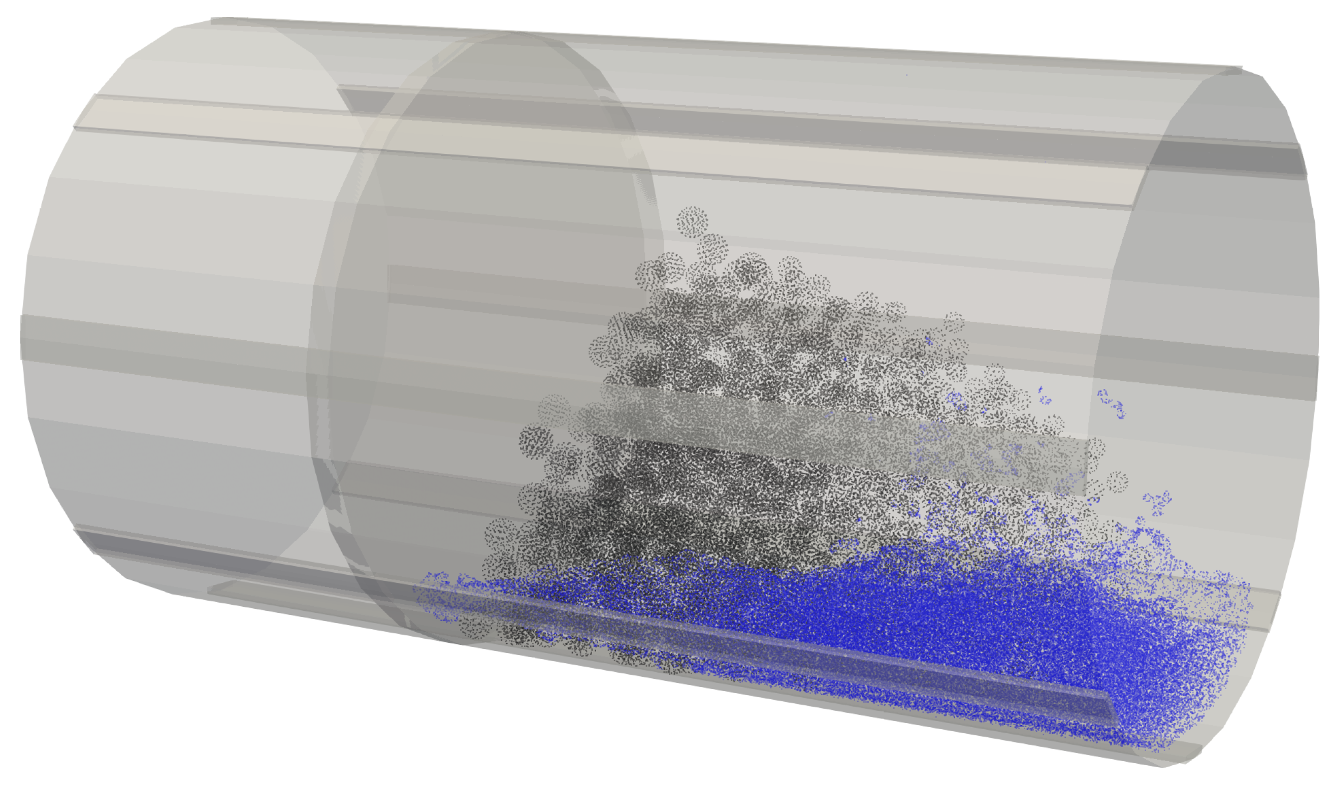
3.8. DualSPHysics Simulation

Simulation in DualSPHysics is set up by defining XML file. Files contain a few important parts, such as the constants definition, parameter definition, geometry definition, movement definition, and definition of the material parameters. Constants and parameters needed to run the simulation are shown below (

Table 1. Material parameters and constants in simulation.

Constant	Value	Description
Lattice	1 (bound), 2 (fluid)	Type of lattice to create initial particles
Gravity	z = −9.81	Gravitational acceleration, m/${\mathrm{s}}^2$
Reference Density (${\rho }_0$)	1400.0	Reference density of the fluid, kg/${\mathrm{m}}^3$
Density Gradient	Rho0	Initial density gradient method
HSWL	0.8 (dry), Auto (wet)	Max still water level for sound speed calculation.
$\gamma$	7 (default)	Polytropic constant for water
System Speed	Auto	Max system speed for calculations
Coef. of Sound	20 (default)	Coefficient to multiply system speed
Sound Speed	Auto	Speed of sound in the simulation
Coef. h	0.15 (dry) 0.8 (wet)	Coefficient for smoothing length calculation
CFL Number	0.2	Coefficient to multiply dt

shows the material parameters, and

Table 2. Parameters and settings of the simulation process.

Parameter	Value	Description
SavePosDouble	0 (default)	Precision for saving particle position
Boundary	DBC	Boundary method used
Step Algorithm	Verlet	Step algorithm for integration
Verlet Steps	40 (default)	Steps for Eulerian equations in Verlet
Kernel	Wendland	Interaction kernel type
Visco Treatment	Artificial	Viscosity formulation
Viscosity ($\nu$)	$8.1·{10}^{-6}$	Viscosity value ${\mathrm{m}}^2$/s
Visco Bound Factor	0.1	Multiplier for boundary viscosity
Density Diffusion Term	Fourtakas	Method for density diffusion
DDT Value	0.1 (default)	Value for density diffusion term
Shifting	Full	Shifting mode for corrections
Shift Coef	−2 (default)	Coefficient for shifting computation
Shift TFS	2.75 (default)	Threshold to detect free surface
Rigid Algorithm	DEM	Algorithm for rigid body dynamics
DtFixed	$1·{10}^{-5}$ s	Fixed time step value, s
DtAllParticles	1	Inclusion of particles for DT calc.
TimeOut	0.01 s	Time out for data output, s
PartsOutMax	1%	Max fluid particles out of domain
RhopOutMin	700 kg/${\mathrm{m}}^3$	Minimum valid density
RhopOutMax	2000 kg/${\mathrm{m}}^3$	Maximum valid density

shows the simulation settings).

Parameters were selected by varied trial-and-error testing to achieve the stability of the simulation for this specific use case and scale. Material properties for each “bound” (boundary) and “float” (free moving body) were set as steel with a Poisson ratio of 0.29 and Young modulus of $1·{10}^8$ Pa. The Young modulus was reduced to achieve more efficient simulation times. The decrease in the Young modulus was balanced by further calibration. Due to DEM calculations in the simulation, a fixed time step was used because it was observed to provide the best stability and fewest errors during calculations.

3.8.1. Geometry Definition

Geometry in the simulation environment has to be defined also in the XML script. Simplified geometry was used to represent the mill and lifters. The mill was defined as a cylinder, and lifters as boxes with proper dimensions. The resolution of discrete particles was defined as 0.005 m. It is the distance between discrete particles, representing all bodies and liquids in the simulation. To resolve the problem of sphere and liquid packing in the limited space in the initial state of the simulation, the mill was modeled as a long cylinder (Figure 15).

Script in Python was developed to generate the particles and liquid in such a way that they would not overlap anything else and not cause errors when populating the geometry with discrete particles.

One of the mill walls was defined as a moving part that, during the first 2 s of the simulation, pushed all of the load into the final volume of the mill, representing the real volume of the laboratory mill used in experiments. Those first 2 s of the simulation were not taken into account during any analysis. Each simulation had 12 s (2 s for wall movement and 10 s of normal mill work).

The geometry is defined through a range of points creating a bounded area and specific shapes like cylinders and boxes to represent the physical environment and objects within the simulation. The point reference serves as the origin, while ‘pointmin’ and ‘pointmax’ define the extents of the simulation domain. Objects are created using commands like ‘drawcylinder’ and ‘drawbox’, with various attributes such as radius, size, and orientation (through rotation angles) to model the simulation environment accurately.

Motion is applied to objects using the ‘<motion>’ section, specifying the type of movement (rotational and rectilinear), its duration, speed, and direction. For instance, rotational movement is defined with an angular velocity around a specified axis, while rectilinear motion specifies velocity in the XYZ coordinates. These motions can be applied to different objects, such as a rotating drum or a vertically moving piston, to simulate dynamic interactions within the fluid. Appropriate rotational speed was applied for each case to reflect the real rotational speed from experiments. An example of the movement of objects inside the mill is shown in Figure 16.

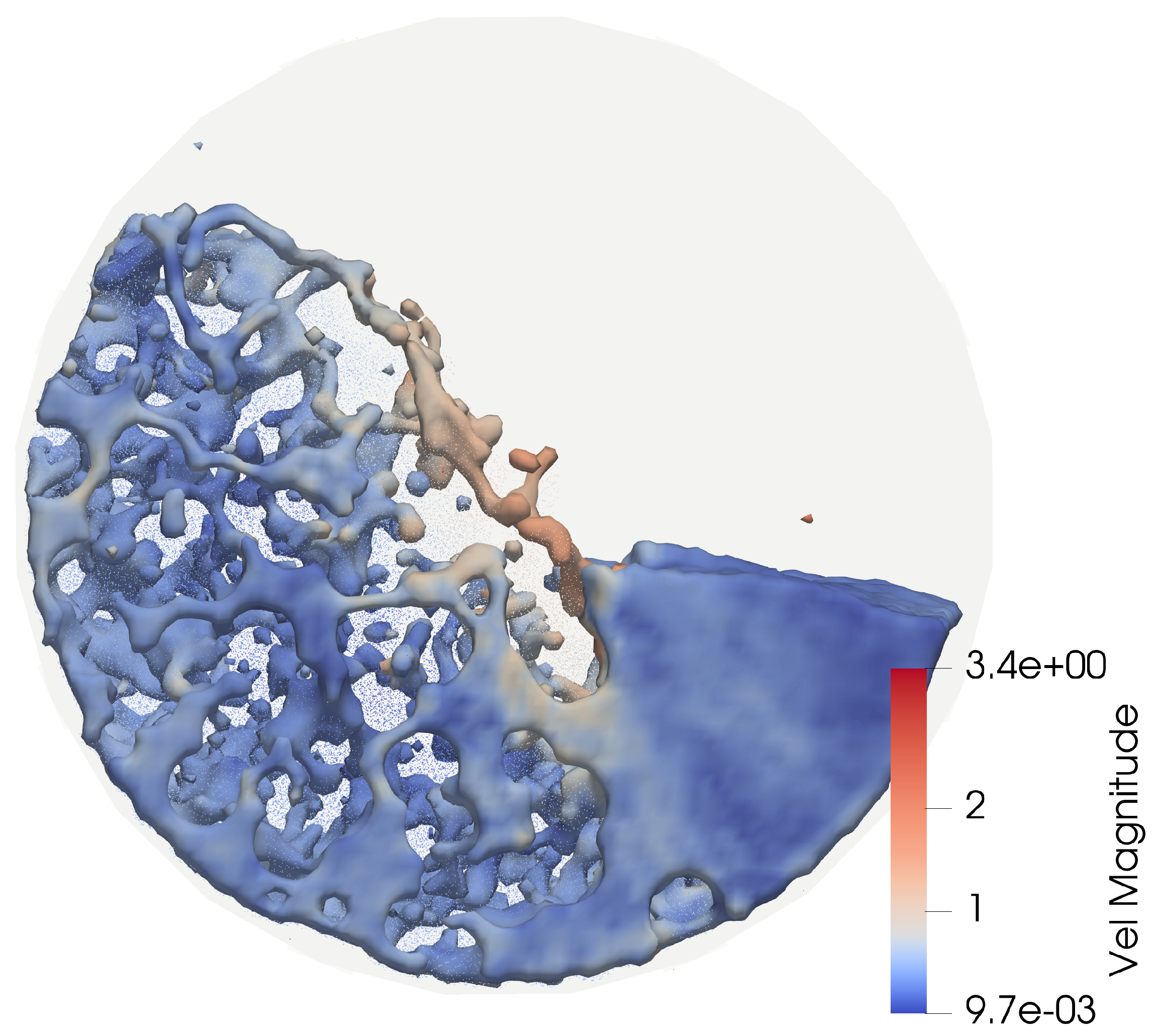
3.8.2. Data Extraction

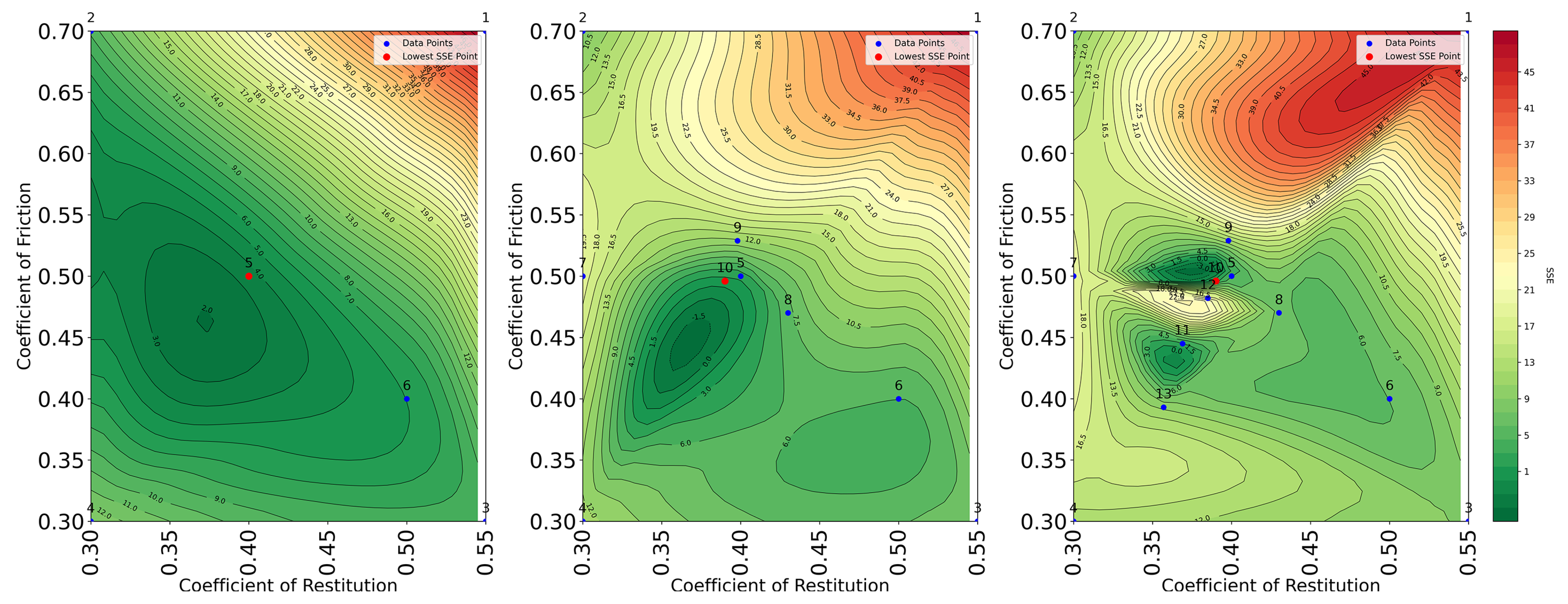
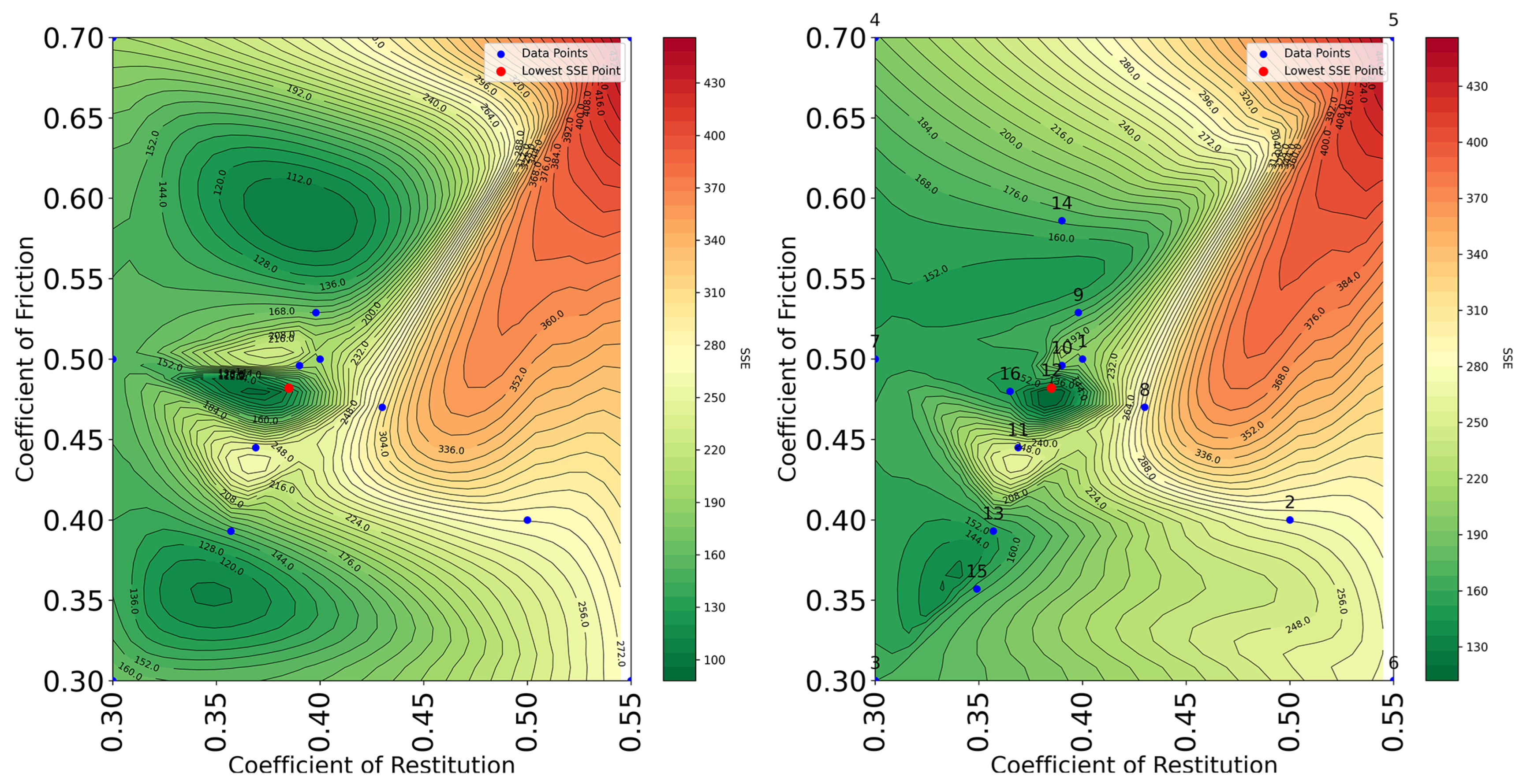
After each simulation, data about ball positions were extracted (Figure 17 (left)) for the sampled time steps. Due to the use of the same lifter heights for all diameters, for the smallest mill diameter, there was a single ball lifter higher than the others on dropped down; this produced the balls seen in the air. For that reason, the heatmap (Figure 17 (right)) showing the most frequent position of the ball charge was created to decrease the impact of those lifted balls on the overall measurement of the angle. This phenomenon occurred in the recordings and simulation, so the same further analysis flow was used for comparable results.

Additionally, for wet milling simulations, additional data about water elevation were extracted. The data were extracted from the plane in the middle of the mill parallel to the front and back walls. The data represented the highest coordinate vertical for each horizontal coordinate on the plane. Due to the discretization of the liquid and representing it with low resolution, there were a lot of outliers. To clean the data and make them more uniform, and reduce the recording of the splashed liquid into the air or the lack of liquid height, because of the low resolution and space occupied in the plane by the steel balls, for each horizontal coordinate (x), the medial position and Q3 were calculated, and only points between those values were taken into account in further curve fitting. Similar to the recording quadratic equation curve approach, a 95% confidence interval was calculated. Figure 18 shows the final load on the mill space after the data extraction process.

3.9. Calibration

For both cases without liquid, only balls with a non-iterative approach were chosen. The behavior of DEM bodies (floats) was modified by changing two parameters: the coefficient of restitution and the coefficient of kinetic friction. Due to the instability of the simulation with higher values, the friction coefficient was explored in the range of 0.3–0.7 and the coefficient of restitution in the range of 0.3–0.55. For each iteration, three simulations with three different mill diameters were performed, and the obtained angles of repose were compared to the ones extracted from the image processing. The sum of square errors (SES) was recorded for each iteration. The ball calibration data from the first six iterations and coefficients and SSE combinations were used to interpolate values between the points. Then, the calibration algorithm was such that the following combination of coefficients tested would be a combination of the coefficients that gave the lowest SSE in the interpolated space. The algorithm was stopped when the three following combinations did not provide a better outcome than the previous combination.

The entire sets of data thus measured angles from simulations from ball calibration were still valuable for calibrating the balls with ore because the ore was not simulated separately; the contact parameters were planned to adjust for the different load behaviors represented by the steel balls. All obtained angles were compared to the ones measured from dry milling recordings to obtain the initial interpolated response surface. The algorithm was later the same. We explored combinations that lowered SSE until three subsequent tests did not give the best result.

As mentioned previously, wet milling recordings were taken into account only from the biggest diameter, so wet milling simulations were also performed only on the 500 mm diameter. Calibration of the liquid also required adjusting kernel parameters or viscosity. The behavior of the liquid is satisfying if both curves fit to the liquid surface for the recording and the simulation fits inside each other’s 95% confidence intervals.

4. Results

The measured dynamic angles of repose for recordings of the ball inside the drum are 43.25, 42.15, and 40.35 degrees for 300, 400, and 500 mm, respectively. The dynamic angles recorded during dry milling processes were found to be 54.24 degrees for a 300 mm measurement, 41.97 degrees for 400 mm, and 47.67 degrees for 500 mm, respectively. Those values are less accurate due to the more challenging extraction of the area of the load in the recording and the reflections on the wall, which this method was not resistant to. The curve fitted to the data from the wet milling recording is presented below, in Figure 19.

Calibration of the ball behavior started with six initial measurements of angles for each diameter in the simulation (3 × 6 = 18 initial simulations). New local minimums were discovered until the 10th iteration, after which no new better combination was found. The final parameters for simulation balls were coefficient of restitution = 0.390 and coefficient of kinetic friction = 0.496. In total, 13 iterations resulting in 39 simulations were performed to achieve those results. The results of the ball behavior calibration, as illustrated in Figure 20, are presented through heatmaps depicting the calibration process of ball behavior in a milling environment. These maps elucidate the relationship between two critical parameters: the coefficient of restitution and the coefficient of kinetic friction, across a color gradient that represents the sum of squared errors (SSE). Specifically, the x-axis details the coefficient of restitution, which quantifies the elasticity of collisions, and the y-axis corresponds to the coefficient of kinetic friction, which measures the resistance to motion. Contour lines represent constant SSE values, with the color gradient from green to red indicating ascending SSE values, thus reflecting the fidelity of the simulation parameters to the experimental observations. The optimal parameters are marked and exhibit the lowest SSE, pointing to the most accurate simulation values determined through the iterative calibration process.

For the calibration of the dry milling, all resulting angles were considered to calculate the initial response surface with the new SSE value. In this case, the 12th iteration from the previous calibration resulted in the best result and lowest SSE. Three possible local minima were explored; none gave better results than the previous best combination from the 12th iteration. Thus, the selected parameters were as follows: coefficient of restitution 0.385 and coefficient of kinetic friction 0.482. Those parameters are less accurate because the recording’s measurement of the load’s angle of repose is less precise. The dry milling calibration results are shown in Figure 21, similar to the previous case, as a heatmap.

The extracted water elevation points for all timesteps, cleaned as described before, are presented in Figure 22.

When comparing these data to the data extracted from the recording (Figure 23), we can see that the fitted curves fit inside each other’s confidence intervals, thus signifying that by just adjusting the fluid’s density and viscosity to realistic values, we obtained a nice match in the behavior of the simulated slurry.

5. Discussion

This section delves into our study’s sophisticated methods and significant insights, spotlighting the role of integrating cutting-edge computer vision with DEM-SPH techniques in enhancing the calibration of digital twins for lab ball mills. We aim to highlight the breakthroughs and future possibilities that this research opens up.

5.1. Embracing Advanced Computer Vision

Our work takes a giant leap forward by incorporating the latest computer vision technology, such as Meta’s SAM model, to automate data gathering. This innovation allows us to precisely track and analyze how the ball mill operates under different conditions by looking at the dynamic angle of repose and monitoring the slurry surface. These detailed observations are crucial for fine-tuning the digital twin of the mill. However, we also encountered some hurdles, especially with the limited visibility in wet milling scenarios, pointing to a need for refining these techniques or finding new ways to gather data on such complex systems.

5.2. Advancing DEM-SPH Calibration

In refining the calibration process, we integrated DEM simulations for the grinding media with SPH models for the slurry flow, showcasing the challenge of capturing milling actions accurately. The careful adjustments of the restitution and friction coefficients in the calibration process underscore the importance of these parameters in mimicking the mill’s real-world behavior. Our efforts in fine-tuning these aspects demonstrate the potential of this method in improving simulation precision, especially for copper ore milling, despite the limitations in measuring dry milling conditions and the promising yet challenging calibration of wet milling.

5.3. The Road Ahead for Digital Twin Calibration

Future work should enhance these calibration techniques to encapsulate the full complexity of industrial milling operations under various conditions. This might include new data collection methods and applying advanced technologies like AI to fine-tune model parameters. Achieving a robust calibration is crucial for harnessing the full predictive power of this approach.

5.4. Leveraging Digital Twins for Milling Efficiency

Our research underscores the transformative potential of calibrated digital twins in milling optimization, particularly for copper ore processing. By accurately simulating milling dynamics, we can explore how different operational settings affect efficiency and energy consumption without requiring extensive physical experiments. This opens up possibilities for designing more energy-efficient milling processes, marking a significant step forward for the mineral processing industry.

5.5. Exploring New Research Avenues

The findings also point to several promising areas for future research. Enhancing computer vision for better data accuracy in wet milling, understanding the long-term benefits of digital twin integration on process efficiency, equipment lifespan, and energy consumption, and conducting further experimental and simulation studies to explore the effects of milling parameters are all critical for realizing the full potential of this innovative approach. This work lays a solid foundation for the ongoing refinement of, and significant advancements in, process optimization.

6. Conclusions

This study presents a comprehensive methodology for calibrating the digital twin of a laboratory ball mill, emphasizing the milling of copper ore through the integration of advanced computer vision techniques and the coupling of DEM (Discrete Element Method) with SPH (Smoothed Particle Hydrodynamics) simulations. The calibration process involved meticulously examining the mill’s behavior under various operational scenarios, including dry and wet milling, facilitated by state-of-the-art image processing and the robust DualSPHysics framework. The following conclusions can be drawn from the research conducted:

• Enhanced Calibration Precision: Integrating computer vision for data extraction and applying DEM-SPH simulations for various milling scenarios significantly improved the accuracy of the digital twin’s behavior compared to actual mill operations. This enhanced precision is pivotal for optimizing milling strategies, leading to more efficient processing and energy utilization.
• Optimization of Milling Processes: The calibrated digital twin provides a powerful tool for understanding and optimizing the grinding process. By accurately simulating the dynamics of the grinding media and slurry, the study paves the way for developing milling processes that are energy efficient and capable of producing high-quality milled products. This optimization potential extends beyond copper ore milling to other materials and milling environments.
• Future Research and Applications: While the current study focuses on copper ore milling, the methodology developed has broader applications. Future research can extend this approach to other milling operations, materials, and industrial processes. Additionally, the integration of further advancements in computer vision and machine learning could automate and refine the calibration process, making digital twins even more accurate and valuable across various sectors.
• Contribution to Sustainable Practices: By enabling the optimization of milling operations for energy efficiency and material usage, the study contributes to more sustainable industrial practices. Simulating and predicting the outcomes of various operational parameters without the need for extensive physical testing conserves resources reduces the environmental footprint of mineral processing industries.

In conclusion, this study successfully demonstrates the viability and benefits of calibrating a digital twin for a laboratory ball mill using the novel integration of computer vision and DEM-SPH simulations. The insights gained and the methodology developed contribute significantly to mineral processing and digital twin technology, offering a promising avenue for future advancements in industrial milling operations and beyond. The calibrated digital twin is a testament to the potential of combining traditional engineering with cutting-edge technology to solve complex challenges in mineral processing and material science.

References

1. Farjana, S.H.; Huda, N.; Parvez Mahmud, M.; Saidur, R. A review on the impact of mining and mineral processing industries through life cycle assessment. J. Clean. Prod. 2019, 231, 1200–1217. [Google Scholar] [CrossRef]
2. Cleary, P.W.; Morrison, R.D.; Sinnott, M.D. Prediction of slurry grinding due to media and coarse rock interactions in a 3D pilot SAG mill using a coupled DEM + SPH model. Miner. Eng. 2020, 159, 106614. [Google Scholar] [CrossRef]
3. Al-Thyabat, S.; Nakamura, T.; Shibata, E.; Iizuka, A. Adaptation of minerals processing operations for lithium-ion (LiBs) and nickel metal hydride (NiMH) batteries recycling: Critical review. Miner. Eng. 2013, 45, 4–17. [Google Scholar] [CrossRef]
4. Tohry, A.; Chehreh Chelgani, S.; Matin, S.; Noormohammadi, M. Power-draw prediction by random forest based on operating parameters for an industrial ball mill. Adv. Powder Technol. 2020, 31, 967–972. [Google Scholar] [CrossRef]
5. Fuerstenau, D.; Abouzeid, A.Z. The energy efficiency of ball milling in comminution. Int. J. Miner. Process. 2002, 67, 161–185. [Google Scholar] [CrossRef]
6. Sverak, T.; Baker, C.; Kozdas, O. Efficiency of grinding stabilizers in cement clinker processing. Miner. Eng. 2013, 43-44, 52–57. [Google Scholar] [CrossRef]
7. Bu, X.; Chen, Y.; Ma, G.; Sun, Y.; Ni, C.; Xie, G. Wet and dry grinding of coal in a laboratory-scale ball mill: Particle-size distributions. Powder Technol. 2020, 359, 305–313. [Google Scholar] [CrossRef]
8. Shi, F.; Xie, W. A specific energy-based size reduction model for batch grinding ball mill. Miner. Eng. 2015, 70, 130–140. [Google Scholar] [CrossRef]
9. Ogonowski, S.; Wołosiewicz-Głąb, M.; Ogonowski, Z.; Foszcz, D.; Pawełczyk, M. Comparison of Wet and Dry Grinding in Electromagnetic Mill. Minerals 2018, 8, 138. [Google Scholar] [CrossRef]
10. He, M.; Wang, Y.; Forssberg, E. Slurry rheology in wet ultrafine grinding of industrial minerals: A review. Powder Technol. 2004, 147, 94–112. [Google Scholar] [CrossRef]
11. Breitung-Faes, S.; Kwade, A. Mill, material, and process parameters—A mechanistic model for the set-up of wet-stirred media milling processes. Adv. Powder Technol. 2019, 30, 1425–1433. [Google Scholar] [CrossRef]
12. Chelgani, S.C.; Parian, M.; Parapari, P.S.; Ghorbani, Y.; Rosenkranz, J. A comparative study on the effects of dry and wet grinding on mineral flotation separation–a review. J. Mater. Res. Technol. 2019, 8, 5004–5011. [Google Scholar] [CrossRef]
13. Kotake, N.; Kuboki, M.; Kiya, S.; Kanda, Y. Influence of dry and wet grinding conditions on fineness and shape of particle size distribution of product in a ball mill. Adv. Powder Technol. 2011, 22, 86–92. [Google Scholar] [CrossRef]
14. Cleary, P.W.; Morrison, R.D. Prediction of 3D slurry flow within the grinding chamber and discharge from a pilot scale SAG mill. Miner. Eng. 2012, 39, 184–195. [Google Scholar] [CrossRef]
15. Morrell, S. Modelling the influence on power draw of the slurry phase in Autogenous (AG), Semi-autogenous (SAG) and ball mills. Miner. Eng. 2016, 89, 148–156. [Google Scholar] [CrossRef]
16. Sinnott, M.; Cleary, P.; Morrison, R. Combined DEM and SPH simulation of overflow ball mill discharge and trommel flow. Miner. Eng. 2017, 108, 93–108. [Google Scholar] [CrossRef]
17. Mayank, K.; Malahe, M.; Govender, I.; Mangadoddy, N. Coupled DEM-CFD Model to Predict the Tumbling Mill Dynamics. Procedia IUTAM 2015, 15, 139–149. [Google Scholar] [CrossRef]
18. Soleymani, M.M.; Fooladi, M.; Rezaeizadeh, M. Effect of slurry pool formation on the load orientation, power draw, and impact force in tumbling mills. Powder Technol. 2016, 287, 160–168. [Google Scholar] [CrossRef]
19. Yin, Z.; Peng, Y.; Zhu, Z.; Ma, C.; Yu, Z.; Wu, G. Effect of mill speed and slurry filling on the charge dynamics by an instrumented ball. Adv. Powder Technol. 2019, 30, 1611–1616. [Google Scholar] [CrossRef]
20. Yuan, C.; Wu, C.; Fang, X.; Liao, N.; Tong, J.; Yu, C. Effect of Slurry Concentration on the Ceramic Ball Grinding Characteristics of Magnetite. Minerals 2022, 12, 1569. [Google Scholar] [CrossRef]
21. Xie, C.; Ma, H.; Song, T.; Zhao, Y. DEM investigation of SAG mill with spherical grinding media and non-spherical ore based on polyhedron-sphere contact model. Powder Technol. 2021, 386, 154–165. [Google Scholar] [CrossRef]
22. Dubé, O.; Alizadeh, E.; Chaouki, J.; Bertrand, F. Dynamics of non-spherical particles in a rotating drum. Chem. Eng. Sci. 2013, 101, 486–502. [Google Scholar] [CrossRef]
23. Tang, J.; Yu, W.; Chai, T.; Liu, Z.; Zhou, X. Selective ensemble modeling load parameters of ball mill based on multi-scale frequency spectral features and sphere criterion. Mech. Syst. Signal Process. 2016, 66–67, 485–504. [Google Scholar] [CrossRef]
24. Senapati, P.; Mishra, B.; Parida, A. Modeling of viscosity for power plant ash slurry at higher concentrations: Effect of solids volume fraction, particle size and hydrodynamic interactions. Powder Technol. 2010, 197, 1–8. [Google Scholar] [CrossRef]
25. Roco, M.; Shook, C. Modeling of slurry flow: The effect of particle size. Can. J. Chem. Eng. 1983, 61, 494–503. [Google Scholar] [CrossRef]
26. Lakhdissi, E.M.; Fallahi, A.; Guy, C.; Chaouki, J. Effect of solid particles on the volumetric gas liquid mass transfer coefficient in slurry bubble column reactors. Chem. Eng. Sci. 2020, 227, 115912. [Google Scholar] [CrossRef]
27. Zhang, X.; Ahmadi, G. Eulerian–Lagrangian simulations of liquid-gas-solid flows in three-phase slurry reactors. Chem. Eng. Sci. 2005, 60, 5089–5104. [Google Scholar] [CrossRef]
28. Buszko, M.H.; Krella, A.K. An Influence of Factors of Flow Condition, Particle and Material Properties on Slurry Erosion Resistance. Adv. Mater. Sci. 2019, 19, 28–53. [Google Scholar] [CrossRef]
29. Olhero, S.; Ferreira, J. Influence of particle size distribution on rheology and particle packing of silica-based suspensions. Powder Technol. 2004, 139, 69–75. [Google Scholar] [CrossRef]
30. Zhang, J.; Zhao, H.; Wang, C.; Li, W.; Xu, J.; Liu, H. The influence of pre-absorbing water in coal on the viscosity of coal water slurry. Fuel 2016, 177, 19–27. [Google Scholar] [CrossRef]
31. Senapati, P.K.; Panda, D.; Parida, A. Predicting viscosity of limestone–water slurry. J. Miner. Mater. Charact. Eng. 2009, 8, 203. [Google Scholar] [CrossRef]
32. Gillies, R.G.; Shook, C.A. Modelling high concentration settling slurry flows. Can. J. Chem. Eng. 2000, 78, 709–716. [Google Scholar] [CrossRef]
33. Andersson, V.; Gudmundsson, J.S. Flow properties of hydrate-in-water slurries. Ann. N. Y. Acad. Sci. 2000, 912, 322–329. [Google Scholar] [CrossRef]
34. Domínguez, J.M.; Fourtakas, G.; Altomare, C.; Canelas, R.B.; Tafuni, A.; García-Feal, O.; Martínez-Estévez, I.; Mokos, A.; Vacondio, R.; Crespo, A.J.C.; et al. DualSPHysics: From fluid dynamics to multiphysics problems. Comput. Part. Mech. 2021, 9, 867–895. [Google Scholar] [CrossRef]
35. Shadloo, M.; Oger, G.; Le Touzé, D. Smoothed particle hydrodynamics method for fluid flows, towards industrial applications: Motivations, current state, and challenges. Comput. Fluids 2016, 136, 11–34. [Google Scholar] [CrossRef]
36. Gotoh, H.; Khayyer, A. On the state-of-the-art of particle methods for coastal and ocean engineering. Coast. Eng. J. 2018, 60, 79–103. [Google Scholar] [CrossRef]
37. Mogan, S.C.; Chen, D.; Hartwig, J.; Sahin, I.; Tafuni, A. Hydrodynamic analysis and optimization of the Titan submarine via the SPH and Finite—Volume methods. Comput. Fluids 2018, 174, 271–282. [Google Scholar] [CrossRef]
38. Manenti, S.; Wang, D.; Domínguez, J.M.; Li, S.; Amicarelli, A.; Albano, R. SPH Modeling of Water-Related Natural Hazards. Water 2019, 11, 1875. [Google Scholar] [CrossRef]
39. Domínguez, J.M.; Crespo, A.J.C.; Gómez-Gesteira, M.; Marongiu, J.C. Neighbour lists in smoothed particle hydrodynamics. Int. J. Numer. Methods Fluids 2011, 67, 2026–2042. [Google Scholar] [CrossRef]
40. Domínguez, J.M.; Crespo, A.J.; Gómez-Gesteira, M. Optimization strategies for CPU and GPU implementations of a smoothed particle hydrodynamics method. Comput. Phys. Commun. 2013, 184, 617–627. [Google Scholar] [CrossRef]
41. Dehnen, W.; Aly, H. Improving convergence in smoothed particle hydrodynamics simulations without pairing instability. Mon. Not. R. Astron. Soc. 2012, 425, 1068–1082. [Google Scholar] [CrossRef]
42. Liu, M.; Liu, G.; Lam, K. Constructing smoothing functions in smoothed particle hydrodynamics with applications. J. Comput. Appl. Math. 2003, 155, 263–284. [Google Scholar] [CrossRef]
43. Monaghan, J.J. Smoothed Particle Hydrodynamics. Annu. Rev. Astron. Astrophys. 1992, 30, 543–574. [Google Scholar] [CrossRef]
44. Wendland, H. Piecewise polynomial, positive definite and compactly supported radial functions of minimal degree. Adv. Comput. Math. 1995, 4, 389–396. [Google Scholar] [CrossRef]
45. Robinson, M. Turbulence and Viscous Mixing Using Smoothed Particle Hydrodynamics. Ph.D. Thesis, Monash University, Clayton, Australia, 2010. [Google Scholar]
46. Monaghan, J. Smoothed particle hydrodynamics. Rep. Prog. Phys. 2005, 68, 1703–1759. [Google Scholar] [CrossRef]
47. Violeau, D. Fluid Mechanics and the SPH Method; Oxford University Press: Oxford, UK, 2012. [Google Scholar]
48. Violeau, D.; Rogers, B. Smoothed particle hydrodynamics (SPH) for free-surface flows: Past, present and future. J. Hydraul. Res. 2016, 54, 1–26. [Google Scholar] [CrossRef]
49. Antuono, M.; Colagrossi, A.; Marrone, S. Numerical diffusive terms in weakly-compressible SPH schemes. Comput. Phys. Commun. 2012, 183, 2570–2580. [Google Scholar] [CrossRef]
50. Bonet, J.; Lok, T.S. Variational and momentum preservation aspects of smooth particle hydrodynamic formulations. Comput. Methods Appl. Mech. Eng. 1999, 180, 97–115. [Google Scholar] [CrossRef]
51. Molteni, D.; Colagrossi, A. A simple procedure to improve the pressure evaluation in hydrodynamic context using the SPH. Comput. Phys. Commun. 2009, 180, 861–872. [Google Scholar] [CrossRef]
52. Fourtakas, G.; Dominguez, J.; Vacondio, R.; Rogers, B. Local uniform stencil (LUST) boundary condition for arbitrary 3-D boundaries in parallel smoothed particle hydrodynamics (SPH) models. Comput. Fluids 2019, 190, 346–361. [Google Scholar] [CrossRef]
53. Monaghan, J.; Gingold, R. Shock simulation by the particle method SPH. J. Comput. Phys. 1983, 52, 374–389. [Google Scholar] [CrossRef]
54. Español, P.; Revenga, M. Smoothed dissipative particle dynamics. Phys. Rev. E 2003, 67, 026705. [Google Scholar] [CrossRef] [PubMed]
55. Lo, Y.; Shao, S. Simulation of near-shore solitary wave mechanics by an incompressible SPH method. Appl. Ocean. Res. 2002, 24, 275–286. [Google Scholar] [CrossRef]
56. Colagrossi, A.; Antuono, M.; Souto-Iglesias, A.; Le Touzé, D. Theoretical analysis and numerical verification of the consistency of viscous smoothed-particle-hydrodynamics formulations in simulating free-surface flows. Phys. Rev. E Stat. Nonlinear Soft Matter Phys. 2011, 84, 026705. [Google Scholar] [CrossRef] [PubMed]
57. Gotoh, H.; Shibahara, T.; Sakai, T. Sub-particle-scale Turbulence Model for the MPS Method: Lagrangian flow model for hydraulic engineering. In Advanced Methods for Computational Fluid Dynamics; TIB: Hannover, Germany, 2001. [Google Scholar]
58. Dalrymple, R.; Rogers, B. Numerical modeling of water waves with the SPH method. Coast. Eng. 2006, 53, 141–147. [Google Scholar] [CrossRef]
59. Monaghan, J. Simulating free surface flows with SPH. J. Comput. Phys. 1994, 110, 399–406. [Google Scholar] [CrossRef]
60. Batchelor, G. An Introduction to Fluid Dynamics; Cambridge University Press: Cambridge, UK, 2000. [Google Scholar]
61. Verlet, L. Computer ‘experiments’ on classical fluids. I. Thermodynamical properties of Lennard-Jones molecules. Phys. Rev. 1967, 159, 98–103. [Google Scholar] [CrossRef]
62. Leimkuhler, B.; Matthews, C. Introduction In Molecular Dynamics: With Deterministic and Stochastic Numerical Methods; Springer: Berlin/Heidelberg, Germany, 2015; pp. 1–51. [Google Scholar]
63. Parshikov, A.; Medin, S.; Loukashenko, I.; Milekhin, V. Improvements in SPH method by means of interparticle contact algorithm and analysis of perforation tests at moderate projectile velocities. Int. J. Impact Eng. 2000, 24, 779–796. [Google Scholar] [CrossRef]
64. Monaghan, J.; Kos, A. Solitary waves on a Cretan beach. J. Waterw. Port Coast. Ocean. Eng. 1999, 125, 145–155. [Google Scholar] [CrossRef]
65. Altomare, C.; Crespo, A.; Rogers, B. Numerical modelling of armour block sea breakwater with smoothed particle hydrodynamics. Comput. Struct. 2014, 130, 34–45. [Google Scholar] [CrossRef]
66. Zhang, F.; Crespo, A.; Altomare, C. DualSPHysics: A numerical tool to simulate real breakwaters. J. Hydrodyn. 2018, 30, 95–105. [Google Scholar] [CrossRef]
67. English, A.; Domínguez, J.; Vacondio, R. Modified dynamic boundary conditions (mDBC) for general purpose smoothed particle hydrodynamics (SPH): Application to tank sloshing, dam break and fish pass problems. Comput. Part. Mech. 2021, 9, 1–5. [Google Scholar] [CrossRef]
68. Crespo, A.; Gómez-Gesteira, M.; Dalrymple, R. Boundary conditions generated by dynamic particles in SPH methods. Comput. Mater. Contin. 2007, 5, 173–184. [Google Scholar] [CrossRef]
69. Lind, S.; Xu, R.; Stansby, P.; Rogers, B. Incompressible smoothed particle hydrodynamics for free-surface flows: A generalised diffusion-based algorithm for stability and validations for impulsive flows and propagating waves. J. Comput. Phys. 2012, 231, 1499–1523. [Google Scholar] [CrossRef]
70. Skillen, A.; Lind, S.; Stansby, P.; Rogers, B. Incompressible smoothed particle hydrodynamics (SPH) with reduced temporal noise and generalised Fickian smoothing applied to body–water slam and efficient wave-body interaction. Comput. Methods Appl. Mech. Eng. 2013, 265, 163–173. [Google Scholar] [CrossRef]
71. Canelas, R.B.; Crespo, A.J.; Domínguez, J.M.; Ferreira, R.M.; Gómez-Gesteira, M. SPH-DCDEM model for arbitrary geometries in free surface solid-fluid flows. Comput. Phys. Commun. 2016, 202, 131–140. [Google Scholar] [CrossRef]
72. Brilliantov, N.; Pöschel, T. Granular gases with impact-velocity-dependent restitution coefficient. In Granular Gases; Springer: Berlin/Heidelberg, Germany, 2001; pp. 100–124. [Google Scholar]
73. Cummins, S.; Cleary, P. Using distributed contacts in DEM. Appl. Math. Model. 2011, 35, 1904–1914. [Google Scholar] [CrossRef]
74. Colagrossi, A.; Landrini, M. Numerical simulation of interfacial flows by smoothed particle hydrodynamics. J. Comput. Phys. 2003, 191, 448–475. [Google Scholar] [CrossRef]
75. Koshizuka, S.; Nobe, A.; Oka, Y. Numerical analysis of breaking waves using the moving particle semi-implicit method. Int. J. Numer. Methods Fluids 1998, 26, 751–769. [Google Scholar] [CrossRef]
76. Canelas, R.B.; Domínguez, J.M.; Crespo, A.J.; Gómez-Gesteira, M.; Ferreira, R.M. A Smooth Particle Hydrodynamics discretization for the modelling of free surface flows and rigid body dynamics. Int. J. Numer. Methods Fluids 2015, 78, 581–593. [Google Scholar] [CrossRef]
77. Price, D.J. Modelling discontinuities and Kelvin–Helmholtz instabilities in SPH. J. Comput. Phys. 2008, 227, 10040–10057. [Google Scholar] [CrossRef]
78. Saitoh, T.R.; Makino, J. A density-independent formulation of smoothed particle hydrodynamics. Astrophys. J. 2013, 768, 44. [Google Scholar] [CrossRef]
79. Kuwabara, G.; Kono, K. Restitution coefficient in a collision between two spheres. Jpn. J. Appl. Phys. 1987, 26, 1230. [Google Scholar] [CrossRef]
80. Kruggel-Emden, H.; Simsek, E.; Rickelt, S.; Wirtz, S.; Scherer, V. Review and extension of normal force models for the discrete element method. Powder Technol. 2007, 171, 157–173. [Google Scholar] [CrossRef]
81. Lemieux, M.; Léonard, G.; Doucet, J.; Leclaire, L.A.; Viens, F.; Chaouki, J.; Bertrand, F. Large-scale numerical investigation of solids mixing in a V-blender using the discrete element method. Powder Technol. 2008, 181, 205–216. [Google Scholar] [CrossRef]
82. Vetsch, D. Numerical Simulation of Sediment Transport with Meshfree Methods. Ph.D. Thesis, ETH, Zurich, Switzerland, 2011. [Google Scholar]
83. Hoomans, B. Granular Dynamics of Gas-Solid Two-Phase Flows. Ph.D. Thesis, University of Twente, Enschede, The Netherlands, 2000. [Google Scholar]
84. Francis, W.; Peters, M.C. Data Sheet No.101-Classification, Properties and Units. In Fuels and Fuel Technology, 2nd ed.; Springer: Berlin/Heidelberg, Germany, 1980; pp. 313–319. [Google Scholar] [CrossRef]
85. Dunne, R.M.E. SME Mineral Processing & Extractive Metallurgy Handbook; Society for Mining, Metallurgy & Exploration (SME): Englewood, CO, USA, 2019. [Google Scholar]
86. Bond, F. Crushing and Grinding Calculations; Allis-Chalmers Manufacturing: Milwaukee, WI, USA, 1961. [Google Scholar]
87. Gupta, A.; Yan, D.S. Mineral Processing Design and Operations: An Introduction, 2nd ed.; Elsevier: Amsterdam, The Netherlands, 2016. [Google Scholar]
88. Kirillov, A.; Mintun, E.; Ravi, N.; Mao, H.; Rolland, C.; Gustafson, L.; Xiao, T.; Whitehead, S.; Berg, A.C.; Lo, W.Y.; et al. Segment Anything. arXiv 2023, arXiv:2304.02643. [Google Scholar]
Figure 1. Configuration and compact support of the kernel function (redrawn from [34]).
Minerals 14 00407 g001
Figure 2. Illustration of various particle sets a ∈ P, with P encompassing all particles within the domain (redrawn from [34]).
Minerals 14 00407 g002
Figure 3. Scheme of DEM mechanism. Left—normal interaction; right—tangential interaction. (Redrawn from [71]).
Minerals 14 00407 g003
Figure 4. Ball mill with different drum sizes.
Minerals 14 00407 g004
Figure 5. Viscosity measurement of copper ore slurry.
Minerals 14 00407 g005
Figure 6. Sample ball and ore load.
Minerals 14 00407 g006
Figure 7. Detection of the mill outline (example mill 500 mm).
Minerals 14 00407 g007
Figure 8. Masked, centered and resized image (example mill 500 mm).
Minerals 14 00407 g008
Figure 9. Masks detected with SAM (example mill 500 mm).
Minerals 14 00407 g009
Figure 10. Processing of binary images of mill recording with only balls inside (example mill 500 mm); 1—created set of binary images from detected masks, 2—heatmap created from binary images, 3—heatmap after thresholding, 4—final image after smoothing.
Minerals 14 00407 g010
Figure 11. Detected highest position in the Y direction and line fitted with linear regression to the points.
Minerals 14 00407 g011
Figure 12. Visualization of detected line over one of the frames from recording (example mill 500 mm).
Minerals 14 00407 g012
Figure 13. Processing of binary images of mill recording of dry milling (example mill 500 mm); 1—created set of binary images from detected masks, 2—heatmap created from binary images, 3—heatmap after thresholding, 4—final image after smoothing.
Minerals 14 00407 g013
Figure 14. GUI interface (example mill 500 mm).
Minerals 14 00407 g014
Figure 15. Geometry generation with balls and liquid generation.
Minerals 14 00407 g015
Figure 16. Movement of the mill wall like a piston.
Minerals 14 00407 g016
Figure 17. Spheres position in the simulation (example mill 300 mm) extracted and saved as binary image (on the left) heatmap generated from the images (on the right).
Minerals 14 00407 g017
Figure 18. Load in the final space in the mill in simulation, vel (m/s).
Minerals 14 00407 g018
Figure 19. Points of the slurry surface detected with the GUI, fitted curve, and 95% confidence interval.
Minerals 14 00407 g019
Figure 20. Calibration of balls behavior.
Minerals 14 00407 g020
Figure 21. Calibration of dry milling.
Minerals 14 00407 g021
Figure 22. Points of the slurry surface extracted from the simulation, with fitted curve and 95% confidence interval.
Minerals 14 00407 g022
Figure 23. Comparison of the data from recording and simulation for wet milling calibration.
Minerals 14 00407 g023