Two Inverse Problems Solution by Feedback Tracking Control

Abstract

Two inverse ill-posed problems are considered. The first problem is an input restoration of a linear system. The second one is a restoration of time-dependent coefficients of a linear ordinary differential equation. Both problems are reformulated as auxiliary optimal control problems with regularizing cost functional. For the coefficients restoration problem, two control models are proposed. In the first model, the control coefficients are approximated by the output and the estimates of its derivatives. This model yields an approximating linear-quadratic optimal control problem having a known explicit solution. The derivatives are also obtained as auxiliary linear-quadratic tracking controls. The second control model is accurate and leads to a bilinear-quadratic optimal control problem. The latter is tackled in two ways: by an iterative procedure and by a feedback linearization. Simulation results show that a bilinear model provides more accurate coefficients estimates.

1. Introduction

The problems of restoration of a system input and coefficients arise in various applications such as metrology [1,2,3,4], image processing [5,6], spectroscopy [7], geophysics [8,9], process control [10], engineering [11,12], medicine [13,14], and many others. The identification of the virus spread models, i.e., the restoration of the coefficients of the corresponding differential equations, became crucial in the period of coronavirus pandemic (see, e.g., [15,16]) for constructing reliable forecasts of the pandemic evolution. These problems belong to a wide class of ill-posed (inverse) problems [17,18,19]. The general framework for the solution of these problems is given by the Tikhonov regularization [17], but its specific implementation varies widely depending on the system description, assumptions on the noise etc.

In this paper, we deal with the input and time-varying coefficients restoration problems for a system, modeled by a linear differential equation, based on noisy output measurements. Mathematically, they are formulated as a first-kind operator equations with compact linear operators mapping an input (coefficients) to the output. In practical formulations, it is assumed that both output and input (coefficient) signals belong to Hilbert spaces. Even if the inverse operator exists, it is unbounded [20], which makes an exact solution unstable w.r.t. output measurement errors. In the Tikhonov regularization method, the solution of the original equation is approximated by the solution of a minimization problem for a so-called smoothing functional, constructed as a sum of a squared discrepancy and some stabilizing functional (stabilizer) with a small coefficient (regularization parameter). The main result of Tikhonov [17] is that by a proper choice of a stabilizer and a regularization parameter, the approximate solution tends to the exact one while the measurement noise tends to zero.

Ill-posed problems in general and the problems of input and coefficient restoration, in particular, are tackled in the literature in numerous forms and by numerous approaches which mainly represent specific adaptations of Tikhonov’s regularization: for linear and non-linear systems [21], in the time [22] and in the frequency [23] domains, in statistical [3,24,25] and deterministic [19] formulations, etc. However, to the best knowledge of the author, a challenging problem of restoration of time-dependent coefficients of a high-order linear differential equation was not formulated previously.

In this paper, we adopt an approach developed in the Ekaterinburg (Sverdlovsk) School on Control Theory [22,26,27,28], where an ill-posed problem is reformulated as an optimal control problem with a Tikhonov-type tracking cost functional. Thus, an inverse problem is solved as a direct control problem, and the control realization approximates the input or the coefficients to be restored. Such a solution enjoys both the regularizing properties of the Tikhonov’s functional minimizer and the stability properties of a feedback control.

In this paper, we mainly concentrate on the problem of restoration of time-dependent coefficients of a linear differential equation. However, the input restoration problem is also formulated, and its solution, based on the auxiliary linear-quadratic tracking problem, is presented. It is important both for methodological purposes (the two problems are solved in similar lines), and from the practical point of view (the stable differentiation, which is the particular case of the input restoration, is implemented for solving the coefficient restoration problem). The novel approach, proposed in this paper, implies reformulating the problem of restoration of time-dependent coefficients of a linear differential equation of order n as an input restoration problem for an auxiliary bilinear system of order ${\mathit{n}}^2$. Then, for a bilinear system, an optimal control problem with a Tikhonov-type cost function is posed, where unknown coefficients play the role of control. For a first-order differential equation, such approach was presented in [29].

Thus, an optimal control version of the coefficient restoration problem yields a bilinear-quadratic formulation. This control problem is treated both by a linear-quadratic approximation and in an exact formulation. The approximate approach needs the output derivatives which are approximated by optimal controls in another auxiliary linear-quadratic problem as it was carried out, e.g., in [30]. The exact, bilinear-quadratic, problem is solved by two approaches. The first one comprises an iterative solution of the corresponding Bellman equation based on [31]. In the second one, a feedback linearization [32] is implemented similarly to [33].

2. Input Restoration Problem

2.1. Ill-Posed Problem Formulation

Consider a linear time-invariant system given by a strictly proper transfer function

$$\mathit{G}\left(\mathit{s}\right)={\displaystyle \frac{{\mathit{b}}_1{\mathit{s}}^{\mathit{n}-1}+{\mathit{b}}_2{\mathit{s}}^{\mathit{n}-2}...+{\mathit{b}}_{\mathit{n}-1}\mathit{s}+{\mathit{b}}_{\mathit{n}}}{{\mathit{s}}^{\mathit{n}}+{\mathit{a}}_1{\mathit{s}}^{\mathit{n}-1}+...+{\mathit{a}}_{\mathit{n}-1}\mathit{s}+{\mathit{a}}_{\mathit{n}}}}.$$

(1)

The problem is a stable (w.r.t. measurement noise) restoration of an unknown scalar input $\mathit{u}\left(\mathit{t}\right)$ based on noisy measurements

$$\tilde{\mathit{y}}\left(\mathit{t}\right)=\mathit{y}\left(\mathit{t}\right)+\eta \left(\mathit{t}\right)$$

(2)

of the scalar output $\mathit{y}\left(t\right)$ where

$$\left|\eta \right(\mathit{t}\left)\right|\le \delta ,\mathit{t}\ge 0,$$

(3)

for some $\delta >0$. Mathematically, this means to solve the operator (integral) equation

$$\mathcal{G}\mathit{u}(·)=\tilde{\mathit{y}}(·),$$

(4)

with the compact operator $\mathcal{G}:{\mathit{L}}_2[0,{\mathit{t}}_{\mathit{f}}]\to {\mathit{L}}_2[0,{\mathit{t}}_{\mathit{f}}]$, ${\mathit{t}}_{\mathit{f}}$ is a given time moment. An operator $\mathcal{G}$ can be, for example, an integral operator of optical instrument in the image restoration problem [5], or a convolution operator of a measuring device in the metrological signal restoration problem [1].

As it is acceptable in the literature on the ill-posed problems (see, e.g., [17] and references therein), it is assumed that for $\eta \left(\mathit{t}\right)\equiv 0$, there exists an exact solution

$${\mathit{u}}^0(·)={\mathcal{G}}^{-1}\mathit{y}(·).$$

(5)

It is well known [17] that the Equation (4) represents an ill-posed problem, i.e., the exact solution in the presence of noise ${\mathit{u}}^{\delta }(·)={\mathcal{G}}^{-1}\tilde{\mathit{y}}(·)$ is unstable w.r.t. data errors. The problem is to construct an approximate solution ${\mathit{u}}^{\delta }(·)$ such that

$$\underset{\delta \to 0}{lim}\left|\right|{\mathit{u}}^{\delta }(·)-{\mathit{u}}^0(·)\left|\right|=0,$$

(6)

where

$$\left|\right|\mathit{u}(·)\left|\right|={\left({\displaystyle \underset{0}{\overset{{\mathit{t}}_{\mathit{f}}}{\int }}{\mathit{u}}^2\left(\mathit{t}\right)\mathit{d}\mathit{t}}\right)}^{1/2}.$$

(7)

Remark 1.

In Tikhonov’s regularization method [17], the approximate (regularized) stable solution of the Equation (4) is given by a minimizer ${\mathit{u}}_{\alpha }(·)$ of a smoothing functional which can be chosen as

$${\mathit{M}}^{\alpha }\left(\mathit{u}(·)\right)=\left|\right|\mathcal{G}\mathit{u}(·)-\tilde{\mathit{y}}{(·)\left|\right|}^2+{\alpha \left|\right|\mathit{u}(·)\left|\right|}^2,$$

(8)

where $\alpha >0$ is a regularization parameter. The minimizer ${\mathit{u}}_{\alpha }(·)$ satisfies the integral Euler-Lagrange equation

$${\mathcal{G}}^{*}\mathcal{G}\mathit{u}(·)+\alpha \mathit{u}(·)={\mathcal{G}}^{*}\tilde{\mathit{y}}(·),$$

(9)

where ${\mathcal{G}}^{*}$ is an operator adjoint to $\mathcal{G}$. Explicitly,

$${\mathit{u}}_{\alpha }(·)={\left({\mathcal{G}}^{*}\mathcal{G}+\alpha \mathcal{I}\right)}^{-1}\tilde{\mathit{y}}(·),$$

(10)

where $\mathcal{I}$ is an identity operator. Moreover, [17] $\alpha =\alpha \left(\delta \right)$ exists, such that ${\mathit{u}}^{\delta }(·)={\mathit{u}}_{\alpha \left(\delta \right)}(·)$ satisfies (6).

2.2. Optimal Control Problem Reformulation

The system determined by the transfer function (1) can be represented as a differential equation in an observable canonical form ([34], Ch. 2):

$$\dot{x}=\mathit{A}\mathit{x}+\mathit{b}\mathit{u},$$

(11)

where

$$\mathit{A}=\left[\begin{array}{ccccc}-{\mathit{a}}_1& 1& 0& \cdots & 0\\ -{\mathit{a}}_2& 0& 1& \cdots & 0\\ ⋮& ⋮& ⋮& \ddots & ⋮\\ -{\mathit{a}}_{\mathit{n}-1}& 0& 0& \cdots & 1\\ -{\mathit{a}}_{\mathit{n}}& 0& 0& \cdots & 0\end{array}\right],\mathit{b}=\left[\begin{array}{c}{\mathit{b}}_1\\ {\mathit{b}}_2\\ ⋮\\ {\mathit{b}}_{\mathit{n}}\end{array}\right],{\mathit{x}}_1=\mathit{y}.$$

(12)

For the system (11), consider the linear-quadratic tracking problem with the cost functional

$${\displaystyle {\mathit{J}}_{\alpha }=\underset{0}{\overset{{\mathit{t}}_{\mathit{f}}}{\int }}{\left(\mathit{D}\mathit{x}\left(\mathit{t}\right)-\tilde{\mathit{y}}\left(\mathit{t}\right)\right)}^2\mathit{d}\mathit{t}+\alpha \underset{0}{\overset{{\mathit{t}}_{\mathit{f}}}{\int }}{\mathit{u}}^2\left(\mathit{t}\right)\mathit{d}\mathit{t},}$$

(13)

where

$$\mathit{D}=[1,0,0,...,0],$$

(14)

$\alpha >0$ is a penalty coefficient for the control effort expenditure. The control problem is minimized (13) by a feedback control $\mathit{u}(\mathit{t},\mathit{x})$. Since $\mathcal{G}\mathit{u}(·)=\mathit{y}(·)=\mathit{D}\mathit{x}(·)={\mathit{x}}_1(·)$, the cost (13) coincides with the Tikhonov’s functional (8). Thus, the problem of minimization of a Tikhonov’s smoothing functional can be solved by a time realization of the optimal strategy in the linear-quadratic tracking problem, (11), (13).

The problem (11), (13) is a particular case of a linear-quadratic regulator problem, and its solution is well-known [35]—namely, the optimal feedback strategy is

$${\mathit{u}}_{\alpha }^{*}(\mathit{t},\mathit{x})=-{\displaystyle \frac{1}{2\alpha }}{\mathit{b}}^{\mathit{T}}{\Phi }^{\mathit{T}}({\mathit{t}}_{\mathit{f}},\mathit{t})\left(2{\mathit{R}}_{\alpha }\left(\mathit{t}\right)\Phi ({\mathit{t}}_{\mathit{f}},t)\mathit{x}+{\mathit{r}}_{\alpha }\left(\mathit{t}\right)\right),$$

(15)

where $\Phi (\mathit{t},\tau )$ is the transition matrix of $\dot{x}=\mathit{A}\mathit{x}$. The matrix function ${\mathit{R}}_{\alpha }\left(\mathit{t}\right)$ satisfies the Riccati differential equation

$$\dot{\mathit{R}}=\mathit{R}{\mathit{Q}}_{\alpha }\left(\mathit{t}\right)\mathit{R}-\mathit{S}\left(\mathit{t}\right),\mathit{R}\left({\mathit{t}}_{\mathit{f}}\right)=0,$$

(16)

where

$${\mathit{Q}}_{\alpha }\left(\mathit{t}\right)={\displaystyle \frac{1}{\alpha }}\Phi ({\mathit{t}}_{\mathit{f}},\mathit{t})\mathit{b}{\mathit{b}}^{\mathit{T}}{\Phi }^{\mathit{T}}({\mathit{t}}_{\mathit{f}},\mathit{t})$$

(17)

$$\mathit{S}\left(\mathit{t}\right)={\Phi }^{\mathit{T}}(\mathit{t},{\mathit{t}}_{\mathit{f}}){\mathit{D}}^{\mathit{T}}\mathit{D}\Phi (\mathit{t},{\mathit{t}}_{\mathit{f}}).$$

(18)

The vector function ${\mathit{r}}_{\alpha }\left(\mathit{t}\right)$ satisfies the linear differential equation

$$\dot{\mathit{r}}={\mathit{R}}_{\alpha }\left(\mathit{t}\right){\mathit{Q}}_{\alpha }\left(\mathit{t}\right)\mathit{r}+2{\Phi }^{\mathit{T}}(\mathit{t},{\mathit{t}}_{\mathit{f}}){\mathit{D}}^{\mathit{T}}\tilde{y}\left(\mathit{t}\right),\mathit{r}\left({\mathit{t}}_{\mathit{f}}\right)=0.$$

(19)

Remark 2.

Both functions ${\mathit{u}}_{\alpha }\left(\mathit{t}\right)={\mathit{u}}_{\alpha }^{*}(\mathit{t},\mathit{x}\left(\mathit{t}\right))$, based on the feedback strategy (15), and ${\mathit{u}}_{\alpha }(·)$ given by (10), solve the input restoration problem. However, a feedback solution is simpler from the computational point of view and it is more stable numerically.

2.3. Stable Differentiation Problem

Let the transfer function be

$$\mathit{G}\left(\mathit{s}\right)={\displaystyle \frac{1}{\mathit{s}}},$$

(20)

i.e., the system is the integrator. The integral Equation (4) becomes

$${\displaystyle \underset{0}{\overset{\mathit{t}}{\int }}\mathit{u}\left(\tau \right)\mathit{d}\tau =\tilde{y}\left(\mathit{t}\right)-\tilde{y}\left(0\right),\mathit{t}\in [0,{\mathit{t}}_{\mathit{f}}],}$$

(21)

and the exact solution without measurement noise $\eta \left(\mathit{t}\right)$ is ${\mathit{u}}^0\left(\mathit{t}\right)=\dot{y}\left(\mathit{t}\right)$. Thus, in this case, the signal restoration problem becomes the problem of stable differentiation of a noisy signal. The system can also be described by the differential equation

$$\dot{x}=\mathit{u},\mathit{x}\left(0\right)={\mathit{x}}_0.$$

(22)

The cost functional (13) in the auxiliary tracking problem becomes

$${\displaystyle {\mathit{J}}_{\alpha }=\underset{0}{\overset{{\mathit{t}}_{\mathit{f}}}{\int }}{(\mathit{x}\left(\mathit{t}\right)-\tilde{y}\left(\mathit{t}\right))}^2\mathit{d}\mathit{t}+\alpha \underset{0}{\overset{{\mathit{t}}_{\mathit{f}}}{\int }}{\mathit{u}}^2\left(\mathit{t}\right)\mathit{d}\mathit{t}.}$$

(23)

In the linear-quadratic problem (22)–(23), $\mathit{A}=0$, $\Phi (\mathit{t},\tau )\equiv 1$, $\mathit{b}=1$, $\mathit{D}=1$, and the optimal control (15) is given by

$${\mathit{u}}_{\alpha }^{*}(\mathit{t},\mathit{x})=-{\displaystyle \frac{1}{2\alpha }}\left(2{\mathit{R}}_{\alpha }\left(\mathit{t}\right)\mathit{x}+{\mathit{r}}_{\alpha }\left(\mathit{t}\right)\right).$$

(24)

The differential Equation (16) for ${\mathit{R}}_{\alpha }\left(\mathit{t}\right)$ becomes

$$\dot{\mathit{R}}={\displaystyle \frac{1}{\alpha }}{\mathit{R}}^2-1,\mathit{R}\left({\mathit{t}}_{\mathit{f}}\right)=0.$$

(25)

By simple algebra, the Equation (25) admits the explicit solution

$${\mathit{R}}_{\alpha }\left(\mathit{t}\right)={\displaystyle \frac{1}{\mu }}tanh\left(\mu ({\mathit{t}}_{\mathit{f}}-\mathit{t})\right),$$

(26)

where

$$\mu \triangleq {\displaystyle \frac{1}{\sqrt{\alpha }}}.$$

(27)

The Equation (19) for ${\mathit{r}}_{\alpha }\left(\mathit{t}\right)$ becomes

$$\dot{r}=\mu tanh\left(\mu ({\mathit{t}}_{\mathit{f}}-\mathit{t})\right)+2\tilde{y}\left(\mathit{t}\right),\mathit{r}\left({\mathit{t}}_{\mathit{f}}\right)=0,$$

(28)

and finds the solution

$${\mathit{r}}_{\alpha }\left(\mathit{t}\right)=-{\displaystyle \frac{{\displaystyle 2\underset{\mathit{t}}{\overset{{\mathit{t}}_{\mathit{f}}}{\int }}cosh\left(\mu ({\mathit{t}}_{\mathit{f}}-\tau )\right)}}{cosh\left(\mu ({\mathit{t}}_{\mathit{f}}-\mathit{t})\right)}}.$$

(29)

By substituting (26) and (29) into the optimal control (15), by integrating the differential Equation (22) for $\mathit{u}={\mathit{u}}_{\alpha }^{*}(\mathit{t},\mathit{x})$ and by assuming that the function $\mathit{y}\left(\mathit{t}\right)$ is twice continuously differentiable, the differentiation error is derived explicitly as

$${\Delta }_{\alpha }\left(\mathit{t}\right)\triangleq {\mathit{u}}_{\alpha }^{*}(\mathit{t},\mathit{x}\left(\mathit{t}\right))-\dot{y}\left(\mathit{y}\right)={\displaystyle \frac{\mu sinh\left(\mu ({\mathit{t}}_{\mathit{f}}-\mathit{t})\right)}{cosh\left(\mu ({\mathit{t}}_{\mathit{f}}-\mathit{t})\right)}}\Delta {\mathit{y}}_0-{\displaystyle \frac{cosh\left(\mu \mathit{t}\right)}{cosh\left(\mu {\mathit{t}}_{\mathit{f}}\right)}}\dot{y}\left({\mathit{t}}_{\mathit{f}}\right)+$$

$${\displaystyle {\displaystyle \frac{cosh\left(\mu \mathit{t}\right)}{cosh\left(\mu {\mathit{t}}_{\mathit{f}}\right)}}\underset{0}{\overset{{\mathit{t}}_{\mathit{f}}}{\int }}cosh\left(\mu ({\mathit{t}}_{\mathit{f}}-\tau )\right)\mathit{w}\left(\tau \right)\mathit{d}\tau -\underset{0}{\overset{\mathit{t}}{\int }}cosh\left(\mu (\mathit{t}-\tau )\right)\mathit{w}\left(\tau \right)\mathit{d}\tau ,}$$

(30)

where

$$\Delta {\mathit{y}}_0=\mathit{y}\left(0\right)-{\mathit{x}}_0,$$

(31)

$$\mathit{w}\left(\mathit{t}\right)=\ddot{\mathit{y}}\left(\mathit{t}\right)-{\mu }^2\eta \left(\mathit{t}\right).$$

(32)

By standard evaluations of the error function (30), the following theorem is established.

Theorem 1.

Let exist ${\mathit{M}}_1>0$ such that

$$|\ddot{y}\left(\mathit{t}\right)|\le {\mathit{M}}_1,t\in [0,{\mathit{t}}_{\mathit{f}}].$$

(33)

Let the penalty coefficient $\alpha =\alpha \left(\delta \right)$ satisfy

$$\underset{\delta \to 0}{lim}\alpha \left(\delta \right)=0,$$

(34)

and exist ${\delta }_0>0$, ${\mathit{M}}_2>0$, such that for $\delta \le {\delta }_0$,

$${\displaystyle \frac{\delta }{\alpha \left(\delta \right)}}\le {\mathit{M}}_2.$$

(35)

Then, for $\delta \to 0$, the realization ${\mathit{u}}_{\alpha }\left(\mathit{t}\right)={\mathit{u}}_{\alpha }^{*}(\mathit{t},\mathit{x}\left(\mathit{t}\right))$ converges to $\dot{y}\left(\mathit{t}\right)$ uniformly on any interval

$[{\epsilon }_1,{\mathit{t}}_{\mathit{f}}-{\epsilon }_2]\subset [0,{\mathit{t}}_{\mathit{f}}]$, ${\epsilon }_1,{\epsilon }_2>0$.

In Figure 1, the results of the feedback differentiation are shown for $\mathit{y}\left(\mathit{t}\right)={\mathit{t}}^2+t+0.1$, ${\mathit{t}}_{\mathit{f}}=2$. The realizations of the functions ${\mathit{R}}_{\alpha }\left(\mathit{t}\right)$ and ${\mathit{r}}_{\alpha }\left(\mathit{t}\right)$ were obtained by a backward numerical integration of differential Equations (25) and (28) with the integration step $\mathit{h}={\displaystyle \frac{2}{N}}$ on the grid ${\mathit{t}}_{\mathit{k}}=\mathit{k}\mathit{h}$, $\mathit{k}=0,1,...,\mathit{N}$, for $\mathit{N}=5000$. Then the Equation (22) was numerically integrated in a forward time. The measurement noise was realized at discrete time moments as random numbers $\eta \left({\mathit{t}}_{\mathit{k}}\right)={\eta }_{\mathit{k}}$ uniformly distributed on $[-\delta ,\delta ]$, $\mathit{k}=0,1,...,\mathit{N}$, for $\delta =0.2$. The results are presented for ${\mathit{x}}_0=0$ and for three values of the penalty coefficient (regularization parameter) $\alpha =\mathit{c}\sqrt{\delta }$ ( $c=0.1,0.02,0.01$) satisfying the conditions of Theorem 1. It is seen that at both ends of the interval $[0,{\mathit{t}}_{\mathit{f}}]$, the error increases.

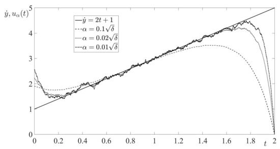
Figure 1. Feedback differentiation of $\mathit{y}\left(\mathit{t}\right)={\mathit{t}}^2+t+0.1.$

The error at the left-hand end of the interval $[0,{\mathit{t}}_{\mathit{f}}]$ is caused by the error in the initial value $\Delta {\mathit{y}}_0\ne 0$. It can be proved that choosing ${\mathit{x}}_0=\tilde{y}\left(0\right)$, for which $|\Delta {\mathit{y}}_0|\le \delta$, guarantees the uniform convergence of ${\mathit{u}}_{\alpha }\left(\mathit{t}\right)$ to $\dot{y}\left(\mathit{t}\right)$ for $\delta \to 0$ on any interval $[0,{\mathit{t}}_{\mathit{f}}-\epsilon ]\subset [0,{\mathit{t}}_{\mathit{f}}]$, $\epsilon >0$.

The error at the right-hand end of $[0,{\mathit{t}}_{\mathit{f}}]$ is caused by the nature of an optimal linear-quadratic control, satisfying ${\mathit{u}}_{\alpha }\left({\mathit{t}}_{\mathit{f}}\right)=0$ independently of the function $\mathit{y}\left(\mathit{t}\right)$, the value of $\delta$ and the value of $\alpha$. We see two possible approaches to circumvent this phenomenon. The first approach is to modify the cost functional by adding a terminal square term:

$${\displaystyle {\overline{J}}_{\alpha }={|\mathit{x}\left({\mathit{t}}_{\mathit{f}}\right)-\overline{x}|}^2+\underset{0}{\overset{{\mathit{t}}_{\mathit{f}}}{\int }}{\left(\mathit{x}\left(\mathit{t}\right)-\tilde{\mathit{y}}\left(\mathit{t}\right)\right)}^2\mathit{d}t+\alpha \underset{0}{\overset{{\mathit{t}}_{\mathit{f}}}{\int }}{\mathit{u}}^2\left(\mathit{t}\right)\mathit{d}\mathit{t},}$$

(36)

where $\overline{\mathit{x}}$ is an additional control parameter. The optimal control in the linear-quadratic problem (22), (36) given by

$${\overline{u}}_{\alpha }(\mathit{t},\mathit{x})=-{\displaystyle \frac{1}{2\alpha }}\left(2{\overline{R}}_{\alpha }\left(\mathit{t}\right)\mathit{x}+{\overline{r}}_{\alpha }\left(\mathit{t}\right)\right),$$

(37)

where ${\overline{R}}_{\alpha }\left(\mathit{t}\right)$ and ${\overline{r}}_{\alpha }\left(\mathit{t}\right)$ satisfy

$$\dot{R}={\displaystyle \frac{1}{\alpha }}{\mathit{R}}^2-1,\mathit{R}\left({\mathit{t}}_{\mathit{f}}\right)=1,$$

(38)

and

$$\dot{r}={\displaystyle \frac{1}{\alpha }}{\mathit{R}}_{\alpha }\left(\mathit{t}\right)\mathit{r}++2\tilde{y}\left(\mathit{t}\right),\mathit{r}\left({\mathit{t}}_{\mathit{f}}\right)=-2\overline{x}.$$

(39)

The second approach comprises extending the control interval from $[0,{\mathit{t}}_{\mathit{f}}]$ to $0,{\mathit{t}}_{\mathit{f}}+\mathit{d}$ for some $\mathit{d}>0$, by extrapolation of the noisy output $\tilde{y}\left(\mathit{t}\right)$ for $\mathit{t}\in [{\mathit{t}}_{\mathit{f}},{\mathit{t}}_{\mathit{f}}+\mathit{d}$. In such a setting, ${\overline{u}}_{\alpha }({\mathit{t}}_{\mathit{f}}+\mathit{d})=0$ and the right-hand error layer shifts to the right.

In Figure 2, the result of above mentioned improvements is presented for the same differentiation problem as in Figure 1 for $\alpha =0.01\sqrt{\delta }$. In this case, the initial condition was ${\mathit{x}}_0=\tilde{y}\left(0\right)$. The control interval was extended to $[0,2.2]$ ( $\mathit{d}=0.2$) by the linear extrapolation based on least squares fitting of $\tilde{y}\left(\mathit{t}\right)$ at the interval $[1.9,2]$. The terminal target point was $\overline{x}=\tilde{\mathit{y}}\left(2.1\right)$. It is seen that the differentiation is more accurate at both ends of the original interval.

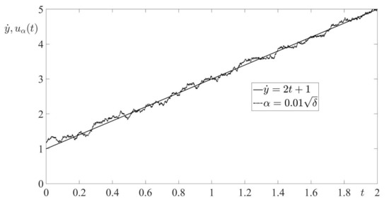
Figure 2. Improved feedback differentiation of $\mathit{y}\left(\mathit{t}\right)={\mathit{t}}^2+t+0.1.$

3. Linear System Coefficients Restoration Problem

3.1. Problem Statement

Consider a linear homogeneous differential equation of order n

$${\mathit{y}}^{\left(\mathit{n}\right)}+{\mathit{u}}_1\left(\mathit{t}\right){\mathit{y}}^{(\mathit{n}-1)}+{\mathit{u}}_2\left(\mathit{t}\right){\mathit{y}}^{(\mathit{n}-2)}+...+{\mathit{u}}_{\mathit{n}-1}\left(\mathit{t}\right){\mathit{y}}^{\prime }+{\mathit{u}}_{\mathit{n}}\left(\mathit{t}\right)\mathit{y}=0,\mathit{t}\in [0,{\mathit{t}}_{\mathit{f}}],$$

(40)

where ${\mathit{u}}_{\mathit{i}}\left(\mathit{t}\right)$, $\mathit{i}=1,...,\mathit{n}$ are the time-dependent coefficients. Let

$$\mathit{y}\left(\mathit{t}\right)={({\mathit{y}}_1\left(\mathit{t}\right),{\mathit{y}}_2\left(\mathit{t}\right),...,{\mathit{y}}_{\mathit{n}}\left(\mathit{t}\right))}^{\mathit{T}},$$

(41)

be the vector of linearly independent solutions ${\mathit{y}}_{\mathit{i}}\left(\mathit{t}\right)$, $\mathit{i}=1,...,\mathit{n}$, of (40). Substituting ${\mathit{y}}_{\mathit{i}}\left(\mathit{t}\right)$, $\mathit{i}=1,...,\mathit{n}$, into (40) yields the linear algebraic system

$${\mathit{H}}_0\left(\mathit{t}\right)\mathit{u}\left(\mathit{t}\right)=-{\mathit{y}}^{\left(\mathit{n}\right)}\left(\mathit{t}\right),$$

(42)

w.r.t. to the coefficients vector

$$\mathit{u}\left(\mathit{t}\right)={({\mathit{u}}_1\left(\mathit{t}\right),{\mathit{u}}_2\left(\mathit{t}\right),...,{\mathit{u}}_{\mathit{n}}\left(\mathit{t}\right))}^{\mathit{T}},$$

(43)

where

$${\mathit{H}}_0\left(\mathit{t}\right)={\left[\begin{array}{cccc}{\mathit{y}}_1\left(\mathit{t}\right)& {\mathit{y}}_2\left(\mathit{t}\right)& ...& {\mathit{y}}_{\mathit{n}}\left(\mathit{t}\right)\\ {\mathit{y}}_1^{\prime }& {\mathit{y}}_2^{\prime }\left(\mathit{t}\right)& ...& {\mathit{y}}_{\mathit{n}}^{\prime }\left(\mathit{t}\right)\\ & & ⋮& \\ {\mathit{y}}_1^{(\mathit{n}-1)}\left(\mathit{t}\right)& {\mathit{y}}_2^{(\mathit{n}-1)}\left(\mathit{t}\right)& ...& {\mathit{y}}_{\mathit{n}}^{(\mathit{n}-1)}\left(\mathit{t}\right)\end{array}\right]}^{\mathit{T}}.$$

(44)

Note that $det{\mathit{H}}_0\left(\mathit{t}\right)$ is equal to the system Wronskian, i.e., $det{\mathit{H}}_0\left(\mathit{t}\right)\ne 0$, and the system (42) admits a unique solution

$${\mathit{u}}^0\left(\mathit{t}\right)=-{\mathit{H}}_0^{-1}\left(\mathit{t}\right){\mathit{y}}^{\left(\mathit{n}\right)}\left(\mathit{t}\right).$$

(45)

However, the problem is to restore the coefficients (43) based on noisy output measurements

$$\tilde{\mathit{y}}\left(\mathit{t}\right)=\mathit{y}\left(\mathit{t}\right)+\eta \left(\mathit{t}\right),\mathit{t}\in [0,{\mathit{t}}_{\mathit{f}}],$$

(46)

where the error vector satisfies

$$\left|\eta \left(\mathit{t}\right)\right|\le \delta ,\mathit{t}\in [0,{\mathit{t}}_{\mathit{f}}],$$

(47)

$\left|\mathit{y}\right|$ denotes the euclidian norm of the vector $\mathit{y}\in {\mathbb{R}}^{\mathit{n}}$. The solution (45) is unstable w.r.t. the measurement noise, even if the exact derivatives of $\mathit{y}\left(\mathit{t}\right)$ are available. Thus, the problem of coefficient restoration is ill-posed and requires regularization.

For the sake of illustration, consider the first-order equation

$$\dot{y}+\mathit{u}\left(\mathit{t}\right)\mathit{y}=0,$$

(48)

yielding the exact solution

$${\mathit{u}}^0\left(\mathit{t}\right)=-{\displaystyle \frac{\dot{y}\left(\mathit{t}\right)}{\mathit{y}\left(\mathit{t}\right)}}.$$

(49)

Assume that the output $\mathit{y}\left(\mathit{t}\right)$ is distorted by a high-frequency noise $\eta \left(\mathit{t}\right)=\delta sin\left(\omega \mathit{t}\right)$ and an exact differentiation is available. Then, the exact solution becomes

$${\mathit{u}}_{\delta }\left(\mathit{t}\right)=-{\displaystyle \frac{\dot{\tilde{\mathit{y}}}\left(\mathit{t}\right)}{\tilde{y}\left(\mathit{t}\right)}}=-{\displaystyle \frac{\dot{y}\left(\mathit{t}\right)+\delta \omega cos\left(\omega \mathit{t}\right)}{\mathit{y}\left(\mathit{t}\right)+\delta sin\left(\omega \mathit{t}\right)}},$$

(50)

which, depending on the values $\delta$ and $\omega$, can yield $\left|\right|\mathit{u}(·)-{\mathit{u}}^0(·)\left|\right|\gg 1$. In Figure 3, the functions (50) and (49) are shown for ${\mathit{u}}^0\left(\mathit{t}\right)=\mathit{t}$ ( $\mathit{y}\left(\mathit{t}\right)=exp(-{\mathit{t}}^2/2)$), $\delta =0.001$, $\omega =1000$. It can be seen that the restoration error is very large.

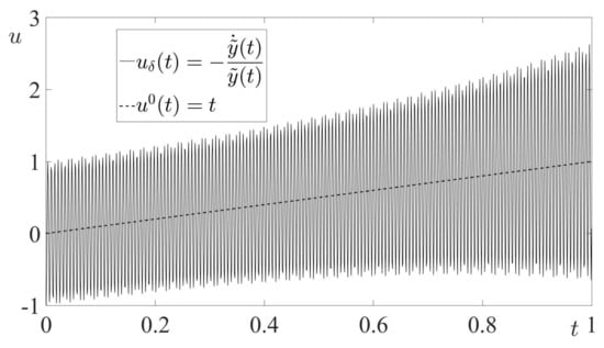
Figure 3. Exact solution is unstable w.r.t. measurement noise.

3.2. Optimal Control Problem Reformulation

Let us introduce a state vector

$$\mathit{x}={({\mathit{x}}_1,{\mathit{x}}_2,...,{\mathit{x}}_{{\mathit{n}}^2})}^{\mathit{T}}\in {\mathbb{R}}^{{\mathit{n}}^2},$$

(51)

where

$${\mathit{x}}_{(\mathit{k}-1)\mathit{n}+\mathit{m}}={\mathit{y}}_{\mathit{k}}^{(\mathit{m}-1)},\mathit{k},\mathit{m}=1,...,\mathit{n}.$$

(52)

Then, for $\eta \left(\mathit{t}\right)\equiv 0$, the system (42) can be rewritten as a bilinear system of differential equations

$$\dot{x}=\mathit{A}\mathit{x}+\mathit{B}\left(\mathit{x}\right)\mathit{u}.$$

(53)

In the Equation (53), A is a block-diagonal ${\mathit{n}}^2\times {\mathit{n}}^2$ matrix

$$\mathit{A}=\left[\begin{array}{ccccc}{\mathit{A}}_0& \mathit{O}& \mathit{O}& \cdots & \mathit{O}\\ \mathit{O}& {\mathit{A}}_0& \mathit{O}& \cdots & \mathit{O}\\ ⋮& ⋮& ⋮& \ddots & ⋮\\ \mathit{O}& \mathit{O}& \mathit{O}& \cdots & {\mathit{A}}_0\end{array}\right],$$

(54)

where ${\mathit{A}}_0$ is the $\mathit{n}\times \mathit{n}$ matrix

$${\mathit{A}}_0=\left[\begin{array}{ccccc}0& 1& 0& ...& 0\\ 0& 0& 1& ...& 0\\ ⋮& ⋮& ⋮& \ddots & ⋮\\ 0& 0& 0& ...& 1\\ 0& 0& 0& ...& 0\end{array}\right].,$$

(55)

O denotes the $\mathit{n}\times \mathit{n}$ zero matrix. The ${\mathit{n}}^2\times \mathit{n}$ matrix $\mathit{B}\left(\mathit{x}\right)$ is

$$\mathit{B}\left(\mathit{x}\right)=\left[\begin{array}{c}{\mathit{B}}_1\left(\mathit{x}\right)\\ {\mathit{B}}_2\left(\mathit{x}\right)\\ ⋮\\ {\mathit{B}}_{\mathit{n}}\left(\mathit{x}\right)\end{array}\right],$$

(56)

where ${\mathit{B}}_{\mathit{k}}\left(\mathit{x}\right)$ are $\mathit{n}\times \mathit{n}$ matrices

$${\mathit{B}}_{\mathit{k}}\left(\mathit{x}\right)=\left[\begin{array}{cccc}0& 0& ...& 0\\ 0& 0& ...& 0\\ ⋮& ⋮& \ddots & ⋮\\ 0& 0& ...& 0\\ -{\mathit{x}}_{(\mathit{k}-1)\mathit{n}+\mathit{n}}& {\mathit{x}}_{(\mathit{k}-1)\mathit{n}+\mathit{n}-1}& ...& -{\mathit{x}}_{(\mathit{k}-1)\mathit{n}+1}\end{array}\right],\mathit{k}=1,...,\mathit{n}.$$

(57)

The output (41) is given by

$$\mathit{y}=\mathcal{F}\left(\mathit{u}\right)={({\mathit{x}}_1,{\mathit{x}}_{\mathit{n}+1},...,{\mathit{x}}_{(\mathit{n}-1)\mathit{n}+1})}^{\mathit{T}}=\mathcal{D}\mathit{x},$$

(58)

where the $\mathit{n}\times {\mathit{n}}^2$ matrix $\mathcal{D}$ is

$$\mathcal{D}=\left[\begin{array}{cccccccccccccc}1& 0& \cdots & 0& & 0& 0& \cdots & 0& \cdots & 0& 0& \cdots & 0\\ 0& 0& \cdots & 0& & 1& 0& \cdots & 0& \cdots & 0& 0& \cdots & 0\\ & & & & & & ⋮& & & & & & \\ 0& 0& \cdots & 0& & 0& 0& \cdots & 0& \cdots & 1& 0& \cdots & 0\end{array}\right].$$

(59)

For example, the second-order differential equation

$$\ddot{\mathit{y}}+{\mathit{u}}_1\left(\mathit{t}\right)\dot{\mathit{y}}+{\mathit{u}}_2\left(\mathit{t}\right)\mathit{y}=0,$$

(60)

having two linearly independent solutions ${\mathit{y}}_1\left(\mathit{t}\right)$ and ${\mathit{y}}_2\left(\mathit{t}\right)$, is represented as a bilinear system of four differential equations for the state vector $\mathit{x}={({\mathit{x}}_1,{\mathit{x}}_2,{\mathit{x}}_3,{\mathit{x}}_4)}^{\mathit{T}}={({\mathit{y}}_1,{\dot{y}}_1,{\mathit{y}}_2,{\dot{y}}_2)}^{\mathit{T}}$:

$$\begin{array}{ccc}{\dot{x}}_1& =& {\mathit{x}}_2\hfill \\ {\dot{x}}_2& =& -{\mathit{x}}_2{\mathit{u}}_1-{\mathit{x}}_1{\mathit{u}}_2,\hfill \\ {\dot{x}}_3& =& x_4\hfill \\ {\dot{x}}_4& =& -{\mathit{x}}_4{\mathit{u}}_1-{\mathit{x}}_3{\mathit{u}}_2,\hfill \end{array}$$

(61)

and the matrices A and $\mathit{B}\left(\mathit{x}\right)$ in (53) are given by (54) and (56) with

$$A_0=\left[\begin{array}{cc}0& 1\\ 0& 0\end{array}\right],{\mathit{B}}_1\left(x\right)=\left[\begin{array}{cc}0& 0\\ -{\mathit{x}}_2& -{\mathit{x}}_1\end{array}\right],{\mathit{B}}_2\left(x\right)=\left[\begin{array}{cc}0& 0\\ -{\mathit{x}}_4& -{\mathit{x}}_3\end{array}\right].$$

(62)

The output is $\mathit{y}={({\mathit{x}}_1,{\mathit{x}}_3)}^{\mathit{T}}$.

Let us formulate for the bilinear system (53) the tracking problem with the cost functional

$${\displaystyle {\mathcal{J}}_{\alpha }=\underset{0}{\overset{{\mathit{t}}_{\mathit{f}}}{\int }}|\mathcal{D}\mathit{x}\left(\mathit{t}\right)-\tilde{y}{\left(\mathit{t}\right)|}^2\mathit{d}\mathit{t}+\alpha \underset{0}{\overset{{\mathit{t}}_{\mathit{f}}}{\int }}{\left|\mathit{u}\left(\mathit{t}\right)\right|}^2\mathit{d}\mathit{t},}$$

(63)

to be minimized by a feedback strategy $\mathit{u}(\mathit{t},\mathit{x})$.

Remark 3.

The cost (63) is the Tikhonov’s regularizing functional. Thus, if ${\mathit{u}}^{*}(\mathit{t},\mathit{x})$ is an optimal feedback in the bilinear-quadratic tracking problem (53), (63), then its time realization ${\mathit{u}}^{*}\left(\mathit{t}\right)={\mathit{u}}^{*}(\mathit{t},\mathit{x}\left(\mathit{t}\right))$ solves the problem of the coefficients restoration. The value of a regularization parameter $\alpha =\alpha \left(\delta \right)$ can be estimated, for example, by employing the discrepancy method [17].

4. Solution of Bilinear-Quadratic Tracking Problem

In this section, several approaches for solving the bilinear-quadratic tracking problem (53), (63) are presented.

4.1. Linear-Quadratic Approximation

In this approach, the matrix $\mathit{B}\left(\mathit{x}\right)$ given by (56), is approximated by the matrix

$$\tilde{B}\left(\mathit{t}\right)=\left[\begin{array}{c}{\tilde{B}}_1\left(\mathit{t}\right)\\ {\tilde{B}}_2\left(\mathit{t}\right)\\ ⋮\\ {\tilde{B}}_{\mathit{n}}\left(\mathit{t}\right)\end{array}\right],$$

(64)

where

$${\tilde{B}}_{\mathit{k}}\left(\mathit{t}\right)=\left[\begin{array}{cccc}0& 0& ...& 0\\ 0& 0& ...& 0\\ ⋮& ⋮& \ddots & ⋮\\ 0& 0& ...& 0\\ -{\tilde{y}}_{\mathit{k}}^{(\mathit{n}-1)}\left(\mathit{t}\right)& -{\tilde{y}}_{\mathit{k}}^{(\mathit{n}-2)}\left(\mathit{t}\right)& ...& -{\tilde{y}}_{\mathit{k}}\left(\mathit{t}\right)\end{array}\right],\mathit{k}=1,...,\mathit{n}.$$

(65)

The approximation (64) and (65) yields a linear system

$$\dot{x}=\mathit{A}\mathit{x}+\tilde{B}\left(\mathit{t}\right)\mathit{u},$$

(66)

approximating the bilinear system (53). Thus, the bilinear-quadratic tracking problem (53), (63) is replaced by an approximating linear-quadratic problem (66), (63).

As it is seen from (65), this approach requires to restore the derivatives of the noisy data $\tilde{y}\left(\mathit{t}\right)$ up to the order $\mathit{n}-1$. In this paper, we use the linear-quadratic differentiation presented in Section 2.3. The advantage of this approach is that the solution of the linear-quadratic tracking problem is well-known. The optimal strategy is similar to (15):

$${\mathit{u}}_{\alpha }^{*}(\mathit{t},\mathit{x})=-{\displaystyle \frac{1}{2\alpha }}\tilde{B}{\left(\mathit{t}\right)}^{\mathit{T}}{\Phi }^{\mathit{T}}({\mathit{t}}_{\mathit{f}},\mathit{t})\left(2{\mathit{R}}_{\alpha }\left(\mathit{t}\right)\Phi ({\mathit{t}}_{\mathit{f}},\mathit{t})\mathit{x}+{\mathit{r}}_{\alpha }\left(\mathit{t}\right)\right),$$

(67)

where the transition matrix $\Phi (\mathit{t},\tau )$ now corresponds to the matrix A given by (54), the matrix function ${\mathit{R}}_{\alpha }\left(\mathit{t}\right)$ satisfies the Riccati differential equation (16), the vector function ${\mathit{r}}_{\alpha }\left(\mathit{t}\right)$ satisfies the linear differential equation (19) with replacing b by $\tilde{B}\left(\mathit{t}\right)$, and D by $\mathcal{D}$.

4.2. Iterative Solution

In this section, a modification of the iterative algorithm, proposed in [31] for a bilinear-quadratic problem with a slightly different cost functional, is applied. Assume that the function ${\mathit{x}}^{\left(0\right)}\left(\mathit{t}\right)$ is given. Then, at each iteration step, the linear-quadratic problem is solved for the system

$${\dot{x}}^{(\mathit{k}+1)}=\mathit{A}{\mathit{x}}^{(\mathit{k}+1)}+\mathit{B}\left({\mathit{x}}^{\left(\mathit{k}\right)}\right)\mathit{u},\mathit{k}=0,1,...$$

(68)

with the cost functional

$${\displaystyle {\mathcal{J}}_{\alpha }^{\mathit{k}+1}=\underset{0}{\overset{t_f}{\int }}|\mathcal{D}{\mathit{x}}^{\mathit{k}+1}\left(\mathit{t}\right)-\tilde{\mathit{y}}{\left(\mathit{t}\right)|}^2\mathit{d}\mathit{t}+\alpha \underset{0}{\overset{{\mathit{t}}_{\mathit{f}}}{\int }}{\left|{\mathit{u}}^{\mathit{k}+1}\left(\mathit{t}\right)\right|}^2\mathit{d}\mathit{t},\mathit{k}=0,1,....}$$

(69)

As in (67), the optimal control in the problem (68) and (69) is

$${\mathit{u}}_{\alpha }^{\mathit{k}+1}(\mathit{t},{\mathit{x}}^{\mathit{k}+1})=-{\displaystyle \frac{1}{2\alpha }}\mathit{B}{\left({\mathit{x}}^{\mathit{k}+1}\right)}^{\mathit{T}}{\Phi }^{\mathit{T}}({\mathit{t}}_{\mathit{f}},\mathit{t})\left(2{\mathit{R}}_{\alpha }^{\mathit{k}+1}\left(\mathit{t}\right)\Phi ({\mathit{t}}_{\mathit{f}},\mathit{t}){\mathit{x}}^{\mathit{k}+1}+{\mathit{r}}_{\alpha }^{\mathit{k}+1}\left(\mathit{t}\right)\right),$$

(70)

where the matrix function ${\mathit{R}}_{\alpha }^{\mathit{k}+1}\left(\mathit{t}\right)$ satisfies the Riccati

$$\dot{R}=\mathit{R}{\mathit{Q}}_{\alpha }^{\left(\mathit{k}\right)}\left(\mathit{t}\right)\mathit{R}-{\mathit{S}}^{\left(\mathit{k}\right)}\left(\mathit{t}\right),\mathit{R}\left({\mathit{t}}_{\mathit{f}}\right)=0,$$

(71)

where

$${\mathit{Q}}_{\alpha }^{\left(\mathit{k}\right)}\left(\mathit{t}\right)={\displaystyle \frac{1}{\alpha }}\Phi ({\mathit{t}}_{\mathit{f}},\mathit{t})\mathit{B}\left({\mathit{x}}^{\left(\mathit{k}\right)}\right){\mathit{B}}^{\mathit{T}}\left({\mathit{x}}^{\left(\mathit{k}\right)}\right){\Phi }^{\mathit{T}}({\mathit{t}}_{\mathit{f}},\mathit{t})$$

(72)

$${\mathit{S}}^{\left(\mathit{k}\right)}\left(\mathit{t}\right)={\Phi }^{\mathit{T}}(\mathit{t},{\mathit{t}}_{\mathit{f}}){\mathcal{D}}^{\mathit{T}}\mathcal{D}\Phi (\mathit{t},{\mathit{t}}_{\mathit{f}}).$$

(73)

The vector function ${\mathit{r}}_{\alpha }^{(\mathit{k}+1)}\left(\mathit{t}\right)$ satisfies the linear differential equation

$$\dot{r}={\mathit{R}}_{\alpha }\left(\mathit{t}\right){\mathit{Q}}_{\alpha }^{\left(\mathit{k}\right)}\left(\mathit{t}\right)\mathit{r}+2{\Phi }^{\mathit{T}}(\mathit{t},{\mathit{t}}_{\mathit{f}}){\mathcal{D}}^{\mathit{T}}\tilde{y}\left(\mathit{t}\right),\mathit{r}\left({\mathit{t}}_{\mathit{f}}\right)=0.$$

(74)

The convergence of this iterative procedure by an appropriate choosing $\alpha =\alpha \left(\delta \right)$ was proved in [31].

4.3. Feedback Linearization

In this section, the bilinear-quadratic control problem is treated by using feedback linearization [32]. The relative degree of the system (53) w.r.t. to each control ${\mathit{u}}_{\mathit{i}}$, $\mathit{i}=1,...,\mathit{n}$, is n, yielding the full relative degree ${\mathit{n}}^2$ [36] w.r.t. to the vector control u. This implies that the system is exactly feedback linearizabile. Namely, define the auxiliary controls

$${\mathit{U}}_{\mathit{k}}=-{\mathit{x}}_{(\mathit{k}-1)\mathit{n}+\mathit{n}}{\mathit{u}}_1-{\mathit{x}}_{(\mathit{k}-1)\mathit{n}+\mathit{n}-1}{\mathit{u}}_{\mathit{n}-1}-...-{\mathit{x}}_{(\mathit{k}-1)\mathit{n}+1}{\mathit{u}}_1,\mathit{k}=1,...,\mathit{n},$$

(75)

or,

$$\mathit{U}=\overline{\mathit{B}}\left(\mathit{x}\right)\mathit{u},$$

(76)

where $\mathit{U}={({\mathit{U}}_1,...,{\mathit{U}}_{\mathit{n}})}^{\mathit{T}}$,

$$\overline{B}\left(\mathit{x}\right)=\left[\begin{array}{cccc}-{\mathit{x}}_{\mathit{n}}& -{\mathit{x}}_{\mathit{n}-1}& ...& -{\mathit{x}}_1\\ -{\mathit{x}}_{2\mathit{n}}& -{\mathit{x}}_{2\mathit{n}-1}& ...& -{\mathit{x}}_{\mathit{n}+1}\\ ⋮& ⋮& \ddots & ⋮\\ 0& 0& ...& 0\\ -{\mathit{x}}_{{\mathit{n}}^2}& {\mathit{x}}_{{\mathit{n}}^2-1}& ...& -{\mathit{x}}_{{\mathit{n}}^2-\mathit{n}+1}\end{array}\right].$$

(77)

Then, by denoting $\mathit{z}=\mathit{x}$, the system (53) is rewritten as

$$\dot{\mathit{z}}=\mathit{A}\mathit{z}+\widehat{B}\mathit{U},$$

(78)

where

$$\widehat{B}=\left[\begin{array}{ccccc}& & \mathit{O}& & \\ 1& 0& ...& 0& 0\\ & & O& & \\ 0& 1& ...& 0& 0\\ & & O& \\ 0& 0& ...& 0& 1\end{array}\right].$$

(79)

Let us formulate the tracking problem for the linear system (78) with the cost functional

$${\displaystyle {\widehat{\mathcal{J}}}_{\alpha }=\underset{0}{\overset{{\mathit{t}}_{\mathit{f}}}{\int }}|\mathcal{D}\mathit{z}\left(\mathit{t}\right)-\tilde{y}{\left(\mathit{t}\right)|}^2\mathit{d}\mathit{t}+\alpha \underset{0}{\overset{{\mathit{t}}_{\mathit{f}}}{\int }}{\left|\mathit{U}\left(\mathit{t}\right)\right|}^2\mathit{d}\mathit{t}.}$$

(80)

The optimal strategy in the linear-quadratic problem (78), (80) is similar to (67):

$${\widehat{U}}_{\alpha }(\mathit{t},\mathit{z})=-{\displaystyle \frac{1}{2\alpha }}{\widehat{B}}^{\mathit{T}}{\Phi }^{\mathit{T}}({\mathit{t}}_{\mathit{f}},\mathit{t})\left(2{\widehat{R}}_{\alpha }\left(\mathit{t}\right)\Phi ({\mathit{t}}_{\mathit{f}},\mathit{t})\mathit{z}+{\widehat{r}}_{\alpha }\left(\mathit{t}\right)\right),$$

(81)

where the matrix function ${\widehat{R}}_{\alpha }\left(\mathit{t}\right)$ satisfies the Riccati differential Equation (16), the vector function ${\widehat{r}}_{\alpha }\left(\mathit{t}\right)$ satisfies the linear differential Equation (19) with replacing b by $\widehat{B}$, and D by $\mathcal{D}$. Due to (76), the optimal control in the bilinear-quadratic problem is

$${\widehat{u}}_{\alpha }(\mathit{t},\mathit{x})={\overline{B}}^{-1}\left(\mathit{x}\right)\mathit{U}(\mathit{t},\mathit{x}).$$

(82)

Remark 4.

The state variables ${\mathit{x}}_{(\mathit{k}-1)\mathit{n}+1}$, $\mathit{k}=1,...,\mathit{n}$, track the functions ${\mathit{y}}_{\mathit{k}}\left(\mathit{t}\right)$, $\mathit{k}+1,...,\mathit{n}$. Then, the value of $|det(\overline{B}\left(\mathit{x}\right)\left)\right|$ should be close to the wronskian of the linear differential Equation (40), providing the invertibility of the matrix $\overline{B}\left(\mathit{x}\right)$. However, due to the measurement noise in $y\left(t\right)$ and the tracking inaccuracy, this matrix can become singular. In order to avoid inverting a singular matrix, in practice we use

$${\widehat{u}}_{\alpha }(\mathit{t},\mathit{x})={\left(\overline{B}\left(\mathit{x}\right)+\mathit{k}{\mathit{I}}_{\mathit{n}}\right)}^{-1}\mathit{U}(\mathit{t},\mathit{x}),$$

(83)

where ${\mathit{I}}_{\mathit{n}}$ is the unit matrix, the parameter $\mathit{k}>0$ is small enough.

4.4. Numerical Example

Let us consider for example the differential equation

$$\ddot{y}-2(\mathit{t}-1)\dot{y}+{(\mathit{t}-1)}^2\mathit{y}=0,$$

(84)

which linearly independent solutions are ${\mathit{y}}_1=exp(\mathit{t}(\mathit{t}-2)/2)cos\mathit{t}$, ${\mathit{y}}_2=exp(\mathit{t}(\mathit{t}-2)/2)sin\mathit{t}$. In Figure 4 and Figure 5, the results of the coefficients restoration by the linear-quadratic approximation are presented for ${\mathit{t}}_{\mathit{f}}=1$, $\delta =0.001$, $\alpha ={10}^{-7}$. The derivatives ${\dot{y}}_1$, ${\dot{y}}_2$ were restored by using the linear-quadratic differentiation described in Section 2.3.

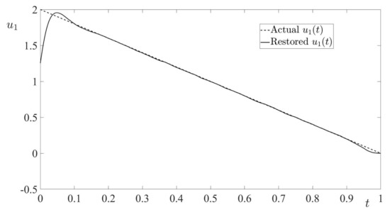
Figure 4. Restoration of ${\mathit{u}}_1\left(\mathit{t}\right)$ by linear-quadratic approximation.

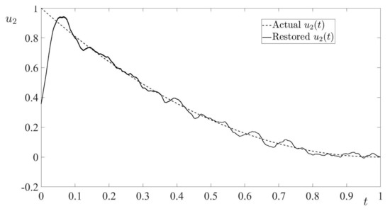
Figure 5. Restoration of ${\mathit{u}}_2\left(\mathit{t}\right)$ by linear-quadratic approximation.

The respective restoration results by using the iterative procedure (for 5 iterations) and feedback linearization are shown in Figure 6, Figure 7, Figure 8 and Figure 9, respectively.

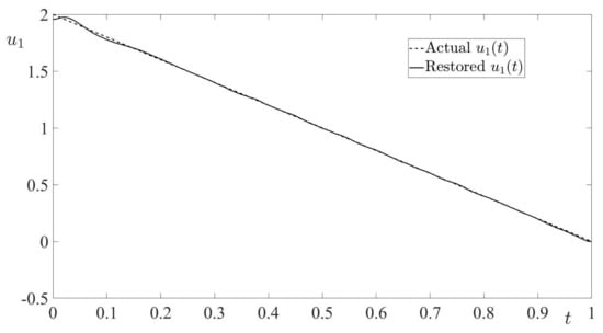
Figure 6. Restoration of ${\mathit{u}}_1\left(\mathit{t}\right)$ by iterations.

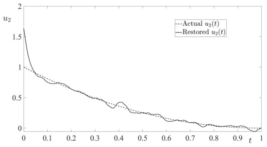
Figure 7. Restoration of ${\mathit{u}}_2\left(\mathit{t}\right)$ by iterations.

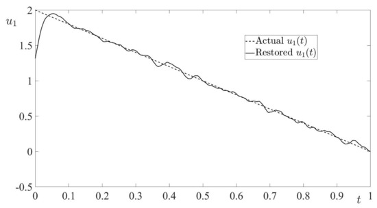
Figure 8. Restoration of ${\mathit{u}}_1\left(\mathit{t}\right)$ by feedback linearization.

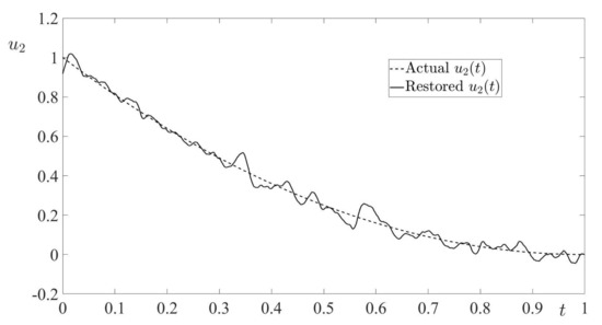
Figure 9. Restoration of ${\mathit{u}}_2\left(\mathit{t}\right)$ by feedback linearization.

Similarly to the differentiation, one can observe the error at the left-hand end ( $\mathit{t}=0$) caused by the inaccuracy in the initial condition.

Let ${\mathit{u}}^{*}\left(\mathit{t}\right)={({\mathit{u}}_1^{*}\left(\mathit{t}\right),{\mathit{u}}_2^{*}\left(\mathit{t}\right))}^{\mathit{T}}$ denote the optimal control time realization, approximating the coefficients $\mathit{u}\left(\mathit{t}\right)$. The restoration ${\mathit{L}}_2$-errors

$${\epsilon }_{\mathit{i}}={\left({\displaystyle \underset{0}{\overset{{\mathit{t}}_{\mathit{f}}}{\int }}{\left({\mathit{u}}_{\mathit{i}}\left(\mathit{t}\right)-{\mathit{u}}_{\mathit{i}}^{*}\left(\mathit{t}\right)\right)}^2\mathit{d}\mathit{t}}\right)}^{1/2},$$

(85)

are presented in Table 1. It is seen that the most accurate restoration of ${\mathit{u}}_1\left(\mathit{t}\right)$ and ${\mathit{u}}_2\left(\mathit{t}\right)$ was obtained by using the iterative algorithm and the feedback linearization, respectively, i.e. by the approaches tackling the original bilinear-quadratic problem.

Table 1. ${\mathit{L}}_2$-errors of restoration.

	${\mathit{u}}_1\left(\mathit{t}\right)$	${\mathit{u}}_2\left(\mathit{t}\right)$
LQ-approximation	$0.07$	$0.08$
Iterative solution	$0.008$	$0.07$
Feedback linearization	$0.07$	$0.03$

5. Conclusions

Two inverse ill-posed problems ((i) input restoration of a linear system and (ii) coefficient restoration of a linear homogeneous differential equation) were considered. Both problems were tackled in a unified manner by reformulating as an optimal control problem with Tikhonov’s cost functional. In both cases, the solution is represented by a feedback control, which adds to the robustness of a proposed approach. The first problem was reformulated as a linear-quadratic tracking problem. A specific attention was paid to a practically important differentiation problem, which solution was further employed in the coefficient restoration. By choosing an initial condition and by modifying the cost functional, the errors at the ends of the time interval were partially circumvented.

The coefficient restoration problem was reformulated as a bilinear-quadratic tracking problem. Three approaches for its solution were proposed: (i) a linear-quadratic approximation, (ii) an iterative method, and (iii) a feedback linearization. In the numerical example, it is shown that the most accurate restoration was obtained by the latter two approaches, tackling an original bilinear-quadratic control problem. The future research should be concentrated in decreasing the errors occurring at the ends of the time interval.

The following abbreviations are used in this manuscript:

References

- Solopchenko, G.N. Inverse problems in measurement. Measurement 1987, 5, 10–19. [Google Scholar] [CrossRef]
- Solopchenko, G.N. Formal metrological components of measuring systems. Measurement 1994, 13, 1–12. [Google Scholar] [CrossRef]
- Aronov, P.M.; Lyashenko, E.A.; Ryashko, L.B. Method of optimum linear-estimation for determining dynamic characteristics of measuring devices. Meas. Tech. 1991, 34, 1091–1096. [Google Scholar] [CrossRef]
- Granovskii, V.A. Models and methods of dynamic measurements: Results presented by St. Petersburg metrologists. In Advanced Mathematical and Computational Tools in Metrology and Testing X; Pavese, F., Bremser, W., Chunovkina, A., Fischer, N., Forbes, A., Eds.; World Scientific Publishing Company: Singapore, 2015; Volume 86, pp. 29–37, Series on Advances in Mathematics for Applied Sciences. [Google Scholar]
- Frieden, B.R. Image enhancement and restoration. In Picture Processing and Digital Filtering; Huang, T.S., Ed.; Springer: New York, NY, USA, 1979. [Google Scholar]
- Bates, R.H.T.; McDonnell, J. Image Restoration and Reconstruction; The Oxford Engineering Science Series; Clarendon Press: Oxford, UK, 1986; Volume 16. [Google Scholar]
- Jansson, P. Deconvolution: With Applications in Spectroscopy; Academic Press: New York, NY, USA, 1984. [Google Scholar]
- Claerbout, J.F. Imaging the Earth’s Interior; Blackwell Scientific Publications: Oxford, UK, 1985. [Google Scholar]
- Prutkin, I. Gravitational and magnetic models of the core-mantle boundary and their correlation. J. Geodyn. 2008, 45, 146–153. [Google Scholar] [CrossRef][Green Version]
- Beck, M.B. Applications of System Identification and Parameter Estimation in Water Quality Modeling; IIASA Working Paper WP-79-099; IIASA: Laxenburg, Austria, 1979. [Google Scholar]
- Isaksson, A.J. Some aspects of industrial system identification. IFAC Proc. Vol. 2013, 46, 153–159. [Google Scholar] [CrossRef]
- Worden, K.; Barthorpe, R.J.; Cross, E.J.; Dervilis, N.; Holmes, G.R.; Manson, G.; Rogers, T.J. On evolutionary system identification with applications to nonlinear benchmarks. Mech. Syst. Signal Process. 2018, 112, 194–232. [Google Scholar] [CrossRef]
- Bellman, R. Mathematical Methods in Medicine; Modern Applied Mathematics; World Scientific: Singapore, 1983; Volume 1. [Google Scholar]
- Schwilden, H.; Honerkamp, J.; Eister, C. Pharmacokinetic model identification and parameter estimation as an ill-posed problem. Eur. J. Clin. Pharmacol. 1993, 45, 545–550. [Google Scholar] [CrossRef] [PubMed]
- Marinov, T.T.; Marinova, R.S. Dynamics of COVID-19 using inverse problem for coefficient identification in SIR epidemic models. Chaos Solitons Fractals X 2020, 5, 1–15. [Google Scholar] [CrossRef]
- Korolev, I. Identification and estimation of the SEIRD epidemic model for COVID-19. J. Econom. 2021, 220, 63–85. [Google Scholar] [CrossRef] [PubMed]
- Tikhonov, A.N.; Arsenin, V.I. Solution of Ill-Posed Problems; John Wiley & Sons: New York, NY, USA, 1977. [Google Scholar]
- Bakushinsky, A.; Goncharsky, A. Ill-Posed Problems: Theory and Applications; Kluwer: Dordrecht, The Netherlands, 1994; Volume 301, Mathematics and Its Applications; [Google Scholar]
- Ivanov, V.; Vasin, V.; Tanana, V. Theory of Linear Ill-Posed Problems and Its Applications; Inverse and Ill-Posed Problems Series; Walter De Gruyter: Berlin, Germany, 2002; Volume 36. [Google Scholar]
- Balakrishnan, A.V. Applied Functional Analysis; Springer: New York, NY, USA, 1976. [Google Scholar]
- Wang, Y.; Yagola, A.M.; Yang, C. (Eds.) Optimization and Regularization for Computational Inverse Problems and Applications; Springer: Berlin/Heidelberg, Germany, 2011. [Google Scholar]
- Kryazhimskiy, A.V.; Osipov, Y.S. Inverse Problems for Ordinary Differential Equations: Dynamical Solutions; Taylor and Francis: Basel, Switzerland, 1995. [Google Scholar]
- Abidi, M.A.; Gribok, A.V.; Paik, J. Frequency-domain implementation of regularization. In Optimization Techniques in Computer Vision: Ill-Posed Problems and Regularization; Springer International Publishing: Cham, Switzerland, 2016; pp. 113–130. [Google Scholar]
- Ljung, L. System Identification (2nd Ed.): Theory for the User; Prentice Hall PTR: Upper Saddle River, NJ, USA, 1999. [Google Scholar]
- Perona, P.; Porporato, A.; Ridolfi, L. On the trajectory method for the reconstruction of differential equations from time series. Nonlinear Dyn. 2000, 23, 13–33. [Google Scholar] [CrossRef]
- Maksimov, V.I. Dynamical identification of unknown characteristics in systems of the second order. In Proceedings of the 2001 European Control Conference, Porto, Portugal, 4–7 September 2001; pp. 1261–1265. [Google Scholar]
- Subbotina, N.N.; Tokmantsev, T.B.; Krupennikov, E.A. On the solution of inverse problems of dynamics of linearly controlled systems by the negative discrepancy method. Proc. Steklov Inst. Math. 2015, 291, 253–262. [Google Scholar] [CrossRef]
- Subbotina, N.N.; Krupennikov, E.A. The method of characteristics in an identification problem. Proc. Steklov Inst. Math. 2017, 299, 205–216. [Google Scholar] [CrossRef]
- Turetsky, V.Y.; Lemsh, E.S. A feedback control in linear system identification. IFAC Proc. Vol. 1996, 29, 1–4. [Google Scholar] [CrossRef]
- Jha, B.; Turetsky, V.; Shima, T. Robust path tracking by a Dubins ground vehicle. IEEE Trans. Control Syst. Technol. 2019, 27, 2614–2621. [Google Scholar] [CrossRef]
- Hofer, E.; Tibker, B. An iterative method for the finite-time bilinear-quadratic control problem. J. Optim. Theory Appl. 1988, 57, 411–427. [Google Scholar] [CrossRef]
- Isidori, A. Nonlinear Control Systems, 2nd ed.; Springer-Verlag: London, UK, 1989. [Google Scholar]
- Turetsky, V. Robust trajectory tracking for a feedback linearizable nonlinear system. IFAC Pap. 2016, 49, 540–545. [Google Scholar] [CrossRef]
- Mellodge, P. A Practical Approach to Dynamical Systems for Engineers; Woodhead Publishing Series in Mechanical Engineering; Elsevier: Amsterdam, The Netherlands, 2016. [Google Scholar]
- Kwakernaak, H.; Sivan, R. Linear Optimal Control Systems; Wiley-Interscience: New York, NY, USA, 1972. [Google Scholar]
- Slotine, J.; Li, W. Applied Nonlinear Control; Prentice Hall: Englewood Cliffs, NJ, USA, 1991. [Google Scholar]
Publisher’s Note: MDPI stays neutral with regard to jurisdictional claims in published maps and institutional affiliations. |
© 2021 by the author. Licensee MDPI, Basel, Switzerland. This article is an open access article distributed under the terms and conditions of the Creative Commons Attribution (CC BY) license (https://creativecommons.org/licenses/by/4.0/).