Modified Viscosity Subgradient Extragradient-Like Algorithms for Solving Monotone Variational Inequalities Problems

Abstract

Variational inequality theory is an effective tool for engineering, economics, transport and mathematical optimization. Some of the approaches used to resolve variational inequalities usually involve iterative techniques. In this article, we introduce a new modified viscosity-type extragradient method to solve monotone variational inequalities problems in real Hilbert space. The result of the strong convergence of the method is well established without the information of the operator’s Lipschitz constant. There are proper mathematical studies relating our newly designed method to the currently state of the art on several practical test problems.

1. Introduction

Assume that $\mathcal{C}$ is a nonempty, closed and convex subset of a real Hilbert space $\mathbb{H}$, and $\mathbb{R}$ and $\mathbb{N}$ are the sets of real numbers and natural numbers, respectively. In this paper, we consider the classical variational inequalities problems [1,2] (in short, $VI(F,\mathcal{C})$) and the solution set of variational inequalities problem represent by $SVI(F,\mathcal{C}).$ Assume that F is an operator $F:\mathbb{H}\to \mathbb{H}$ and the variational inequalities problem for an operator $F:\mathbb{H}\to \mathbb{H}$ is defined in the following way:

$$\mathrm{Find}{u}^{*}\in \mathcal{C}\mathrm{such}\mathrm{that}⟨F\left(u^{*}\right),y-u^{*}⟩\ge 0,\forall y\in \mathcal{C}.$$

(1)

The problem (1) is well defined and equivalent to solve the following fixed point problem:

$$\mathrm{Find}\mathrm{a}\mathrm{point}{u}^{*}\in \mathcal{C}\mathrm{such}\mathrm{that}{u}^{*}=P_{\mathcal{C}}[u^{*}-\zeta F\left(u^{*}\right)],$$

for some $0<\zeta <\frac{1}{L}$ where L is the Lipschitz constant of the operator F. We assume that the followings conditions have been satisfied:

(b1)

The solution set is represented by $SVI(F,\mathcal{C})$ and it is nonempty;

(b2)

An operator $F:\mathbb{H}\to \mathbb{H}$ is monotone—i.e.,

$$⟨F\left(u_1\right)-F\left(u_2\right),u_1-u_2⟩\ge 0,\forall u_1,u_2\in \mathcal{C};$$

(b3)

F is Lipschitz continuous if there exists $L>0$, such that

$$\parallel F\left(u_1\right)-F\left(u_2\right)\parallel \le L\parallel u_1-u_2\parallel ,\forall u_1,u_2\in \mathcal{C}.$$

The variational inequalities theory is a useful technique for investigating a large number of problems in physics, economics, engineering and optimization theory. It was firstly introduced by Stampacchia [1] in 1964 and also well established that the problem (1) is an important problem in nonlinear analysis. It is an advantageous mathematical model that puts together several topics of applied mathematics, such as the network equilibrium problems, the necessary optimality conditions, the systems of non-linear equations and the complementarity problems [3,4,5,6,7].

The projection method and its modified version methods are crucial for finding the numerical solutions of variational inequality problems. Many studies have been suggested and researched different types of projection methods to solve the variational inequalities problem (see for more details [8,9,10,11,12,13,14,15,16,17,18]) and others, as in [19,20,21,22,23,24,25,26,27,28]. The simplistic methodology is the gradient method for which only one projection on a feasible set is required. A convergence of the method, however, requires strong monotonicity on F. To prevent the strong monotonicity hypothesis, Korpelevich [8] and Antipin [29] introduced the following extragradient method.

$$\left\{\begin{array}{c}{u}_n\in \mathcal{C},\hfill \\ v_n=P_{\mathcal{C}}[u_n-\zeta F\left(u_n\right)],\hfill \\ u_{n+1}=P_{\mathcal{C}}[u_n-\zeta F\left(v_n\right)],\hfill \end{array}\right.$$

for some $0<\zeta <\frac{1}{L}$. The subgradient extragradient algorithm was recently developed by Censor et al. [10] to resolve problem (1) in real Hilbert space. Their method has the form of

$$\left\{\begin{array}{c}{u}_n\in \mathcal{C},\hfill \\ v_n=P_{\mathcal{C}}[u_n-\zeta F\left(u_n\right)],\hfill \\ u_{n+1}=P_{{\mathbb{H}}_n}[u_n-\zeta F\left(v_n\right)],\hfill \end{array}\right.$$

(2)

where $0<\zeta <\frac{1}{L}$ and ${\mathbb{H}}_n=\{z\in \mathbb{H}:⟨u_n-\zeta F\left(u_n\right)-v_n,z-v_n⟩\le 0\}.$

In this article, motivated by the methods in [10,30,31] and the viscosity method [14] we introduce a new viscosity subgradient–extragradient algorithm to solve variational inequality problems involving monotone operators in Hilbert space. It is important to note that, our proposed algorithm operates more effectively than the existing ones. Particularly in comparison to the results of Yang et al. [30], our algorithm operates efficiently in most situations. Analogously to the results of Yang et al. [30], proof of the convergence of Algorithm 1, it is not compulsory to have the information of the Lipschitz constant of the operator $F.$ The proposed algorithm could be seen as a modification of the methods that are found in [8,10,30,31]. Under mild conditions, a strong convergence theorem was proven to be associated with the proposed method. Numerical experimental studies have been shown that the new method considers being more effective than the current ones in [30].

The rest of the article is arranged in the following way: Section 2 provides a few definitions and basic results that are used throughout the paper. Section 3 contains the main algorithm and convergence theorem. Section 4 includes the numerical results that illustrate the algorithmic efficacy of the introduced method.

Algorithm 1 An Explicit Method for Monotone Variational Inequality Problems

Step 0: Let $u_0\in \mathcal{C},$$\mu \in (0,1),$${\zeta }_0>0$ and a sequence ${\beta }_n\subset (0,1)$ with ${\beta }_n\to 0$ and ${\sum }_n^{\infty }{\beta }_n=+\infty .$ Step 1: Assume that $\left\{u_n\right\}$ is given and compute $$v_n=P_{\mathcal{C}}[u_n-{\zeta }_{n}F\left(u_n\right)].$$  If $u_n=v_n$; STOP. Else, move to Step 2. Step 2: Create a half-space $${\mathbb{H}}_n=\{z\in \mathbb{H}:⟨u_n-{\zeta }_{n}F\left(u_n\right)-v_n,z-v_n⟩\le 0\}.$$ Step 3: $$u_{n+1}={\beta }_{n}f\left(u_n\right)+(1-{\beta }_n)z_n,$$  while $z_n=P_{{\mathbb{H}}_n}[u_n-{\zeta }_{n}F\left(v_n\right)].$ Step 4: Compute $${\zeta }_{n+1}=\left\{\begin{array}{cc}min\left\{{\zeta }_n,\frac{\mu \parallel u_n-v_n{\parallel }^2+\mu {\parallel z_n-v_n\parallel }^2}{2⟨F\left(u_n\right)-F\left(v_n\right),z_n-v_n⟩}\right\}\mathrm{if}\hfill & ⟨F\left(u_n\right)-F\left(v_n\right),z_n-v_n⟩>0,\hfill \\ {\zeta }_n\hfill & \mathrm{otherwise}.\hfill \end{array}\right.$$  Set $n:=n+1$ and return to Step 1.

2. Background

A metric projection $P_{\mathcal{C}}\left(u_1\right)$ for $u_1\in \mathbb{H}$ onto a closed and convex subset $\mathcal{C}$ of $\mathbb{H}$ is defined by

$$P_{\mathcal{C}}\left(u_1\right)=\underset{}{argmin}\{\parallel u_2-u_1\parallel :u_2\in \mathcal{C}\}.$$

Lemma 1

([32]; Page 31). For $u,v\in \mathbb{H}$ and $a\in \mathbb{R},$ then the following relationship holds.

(i). 

${\parallel au+(1-a)v\parallel }^2={a\parallel u\parallel }^2+{(1-a)\parallel v\parallel }^2-a(1-a){\parallel u-v\parallel }^2.$

(ii). 

${\parallel u+v\parallel }^2\le {\parallel u\parallel }^2+2⟨v,u+v⟩$.

Lemma 2

([32,33]). Assume $\mathcal{C}$ be a nonempty, closed and convex subset of a real Hilbert space $\mathbb{H}$ and let $P_{\mathcal{C}}:\mathbb{H}\to \mathcal{C}$ be a metric projection from $\mathbb{H}$ onto $\mathcal{C}$. Then:

(i). 

Let $u_1\in \mathcal{C}$ and $u_2\in \mathbb{H}$

$$\parallel u_1-P_{\mathcal{C}}\left(u_2\right){\parallel }^2+\parallel P_{\mathcal{C}}\left(u_2\right)-u_2{\parallel }^2\le {\parallel u_1-u_2\parallel }^2.$$

(ii). 

$u_3=P_{\mathcal{C}}\left(u_1\right)$ if and only if

$$⟨u_1-u_3,u_2-u_3⟩\le 0,\forall u_2\in \mathcal{C}.$$

(iii). 

For $u_2\in \mathcal{C}$ and $u_1\in \mathbb{H}$

$$\parallel u_1-P_{\mathcal{C}}\left(u_1\right)\parallel \le \parallel u_1-u_2\parallel .$$

Lemma 3

([34]). Assume that $\left\{{\chi }_n\right\}$ is a sequence of non-negative real numbers such that

$${\chi }_{n+1}\le (1-{\alpha }_n){\chi }_n+{\alpha }_n{\delta }_n,\forall n\in \mathbb{N},$$

where $\left\{{\alpha }_n\right\}\subset (0,1)$ and $\left\{{\delta }_n\right\}\subset \mathbb{R}$ meet with the following criteria:

$$\underset{n\to \infty }{lim}{\alpha }_n=0,\sum _{n=1}^{\infty }{\alpha }_n=\infty ,and\underset{n\to \infty }{lim\; sup}{\delta }_n\le 0.$$

Then, ${lim}_{n\to \infty }{\chi }_n=0.$

Lemma 4

([35]). Assume that $\left\{{\chi }_n\right\}$ is a sequence of real numbers such that there is a subsequence $\left\{n_i\right\}$ of $\left\{n\right\}$ such that ${\chi }_{n_i}<{\chi }_{n_{i+1}}$ for all $i\in \mathbb{N}.$ Then, there is a non decreasing sequence $m_k\subset \mathbb{N}$ such that $m_k\to \infty$ as $k\to \infty ,$ and the following conditions are fullfilled by all (sufficiently large) numbers $k\in \mathbb{N}$:

$${\chi }_{m_k}\le {\chi }_{m_{k+1}}and{\chi }_k\le {\chi }_{m_{k+1}}.$$

In fact, $m_k=max\{j\le k:{\chi }_j\le {\chi }_{j+1}\}.$

Lemma 5

([36]). Assume that $\mathcal{C}$ is a nonempty closed convex set in $\mathbb{H}$ and an operator $F:\mathcal{C}\to \mathbb{H}$ is monotone and continuous. Then, $u^{*}$ is a solution of the problem (1) if and only if $u^{*}$ is a solution of the following problem:

$$Findx\in \mathcal{C}\mathit{such}\mathit{that}⟨F\left(y\right),y-x⟩\ge 0,\forall y\in \mathcal{C}.$$

3. Algorithm and Corresponding Strong Convergence Theorem

We provide a method consisting of two convex minimization problems through a viscosity and an explicit stepsize formula which are being used to enhance the rate of convergence the iterative sequence and to make the method independent of the Lipschitz constant L. The detailed method is given below:

Remark 1.

${\mathbb{H}}_n$ is a half-space and so ${\mathbb{H}}_n$ is a closed and convex set in $\mathbb{H}.$

Lemma 6.

The sequence $\left\{{\zeta }_n\right\}$ is decreasing monotonically with a lower bound $min\left\{\frac{\mu }{L},{\zeta }_0\right\}$ and converges to $\zeta >0.$

Proof. 

From the sequence $\left\{{\zeta }_n\right\},$ we see that this sequence is monotone and nonincreasing. It is given that F is Lipschitz-continuous with $L>0$. Let $⟨F\left(u_n\right)-F\left(v_n\right),z_n-v_n⟩>0,$ such that

$$\begin{array}{cc}\hfill \frac{\mu (\parallel u_n-v_n{\parallel }^2+\parallel z_n-v_n{\parallel }^2)}{2⟨F\left(u_n\right)-F\left(v_n\right),z_n-v_n⟩}& \ge \frac{2\mu \parallel u_n-v_n\parallel \parallel z_n-v_n\parallel }{2\parallel F\left(u_n\right)-F\left(v_n\right)\parallel \parallel z_n-v_n\parallel }\hfill \\ \hfill & \ge \frac{2\mu \parallel u_n-v_n\parallel \parallel z_n-v_n\parallel }{2\parallel u_n-v_n\parallel \parallel z_n-v_n\parallel }\hfill \\ \hfill & \ge \frac{\mu }{L}.\hfill \end{array}$$

(3)

The above discussion implies that the sequence $\left\{{\zeta }_n\right\}$ has a lower bound $min\left\{\frac{\mu }{L},{\zeta }_0\right\}.$ Moreover, there exists number $\zeta >0,$ such that ${lim}_{n\to \infty }{\zeta }_n=\zeta .$  □

Lemma 7.

Assume that an operator $F:\mathcal{C}\to \mathbb{H}$ satisfies the conditions(b1)–(b3). For each $u^{*}\in SVI(F,\mathcal{C})\ne \varnothing ,$ we have

$$\parallel z_n-u^{*}{\parallel }^2\le \parallel u_n-u^{*}{\parallel }^2-\left(1-\frac{\mu {\zeta }_n}{{\zeta }_{n+1}}\right)\parallel u_n-v_n{\parallel }^2-\left(1-\frac{\mu {\zeta }_n}{{\zeta }_{n+1}}\right){\parallel z_n-v_n\parallel }^2.$$

Proof. 

Let consider the following

$$\begin{array}{cc}\hfill {∥z_n-u^{*}∥}^2& ={∥P_{{\mathbb{H}}_n}[u_n-{\zeta }_{n}F\left(v_n\right)]-u^{*}∥}^2\hfill \\ \hfill & ={∥P_{{\mathbb{H}}_n}[u_n-{\zeta }_{n}F\left(v_n\right)]+[u_n-{\zeta }_{n}F\left(v_n\right)]-[u_n-{\zeta }_{n}F\left(v_n\right)]-u^{*}∥}^2\hfill \\ \hfill & ={∥[u_n-{\zeta }_{n}F\left(v_n\right)]-u^{*}∥}^2+{∥P_{{\mathbb{H}}_n}[u_n-{\zeta }_{n}F\left(v_n\right)]-[u_n-{\zeta }_{n}F\left(v_n\right)]∥}^2\hfill \\ \hfill & +2⟨P_{{\mathbb{H}}_n}[u_n-{\zeta }_{n}F\left(v_n\right)]-[u_n-{\zeta }_{n}F\left(v_n\right)],[u_n-{\zeta }_{n}F\left(v_n\right)]-u^{*}⟩.\hfill \end{array}$$

(4)

From the assumption that $u^{*}\in SVI(F,\mathcal{C})\subset \mathcal{C}\subset {\mathbb{H}}_n,$ we have

$$\begin{array}{cc}\hfill & {∥P_{{\mathbb{H}}_n}[u_n-{\zeta }_{n}F\left(v_n\right)]-[u_n-{\zeta }_{n}F\left(v_n\right)]∥}^2\hfill \\ \hfill & +⟨P_{{\mathbb{H}}_n}[u_n-{\zeta }_{n}F\left(v_n\right)]-[u_n-{\zeta }_{n}F\left(v_n\right)],[u_n-{\zeta }_{n}F\left(v_n\right)]-u^{*}⟩\hfill \\ \hfill & =⟨[u_n-{\zeta }_{n}F\left(v_n\right)]-P_{{\mathbb{H}}_n}[u_n-{\zeta }_{n}F\left(v_n\right)],u^{*}-P_{{\mathbb{H}}_n}[u_n-{\zeta }_{n}F\left(v_n\right)]⟩\le 0,\hfill \end{array}$$

(5)

implies that

$$\begin{array}{cc}\hfill & ⟨P_{{\mathbb{H}}_n}[u_n-{\zeta }_{n}F\left(v_n\right)]-[u_n-{\zeta }_{n}F\left(v_n\right)],[u_n-{\zeta }_{n}F\left(v_n\right)]-u^{*}⟩\hfill \\ \hfill & \le -{∥P_{{\mathbb{H}}_n}[u_n-{\zeta }_{n}F\left(v_n\right)]-[u_n-{\zeta }_{n}F\left(v_n\right)]∥}^2.\hfill \end{array}$$

(6)

Now, using the Equation (4) implies that

$$\begin{array}{cc}\hfill \parallel z_n-u^{*}{\parallel }^2& \le {∥u_n-{\zeta }_{n}F\left(v_n\right)-u^{*}∥}^2-{∥P_{{\mathbb{H}}_n}[u_n-{\zeta }_{n}F\left(v_n\right)]-[u_n-{\zeta }_{n}F\left(v_n\right)]∥}^2\hfill \\ \hfill & \le \parallel u_n-u^{*}{\parallel }^2-{\parallel u_n-z_n\parallel }^2+2{\zeta }_n⟨F\left(v_n\right),u^{*}-z_n⟩.\hfill \end{array}$$

(7)

Given that $u^{*}$ is a solution of $VI(F,\mathcal{C})$, we get

$$⟨F\left(u^{*}\right),y-u^{*}⟩\ge 0,\forall y\in \mathcal{C}.$$

(8)

Due to the monotonicity of F on $\mathcal{C}$, we can obtain

$$⟨F\left(v_n\right)-F\left(u^{*}\right),v_n-u^{*}⟩\ge 0,\forall y\in \mathcal{C}.$$

(9)

Since $v_n\in \mathcal{C},$ it follows that

$$⟨F\left(v_n\right),v_n-u^{*}⟩\ge 0.$$

(10)

Thus, we have

$$⟨F\left(v_n\right),u^{*}-z_n⟩=⟨F\left(v_n\right),u^{*}-v_n⟩+⟨F\left(v_n\right),v_n-z_n⟩\le ⟨F\left(v_n\right),v_n-z_n⟩.$$

(11)

From (7) and (11), we get

$$\begin{array}{cc}\hfill \parallel z_n-u^{*}{\parallel }^2& \le \parallel u_n-u^{*}{\parallel }^2-{\parallel u_n-z_n\parallel }^2+2{\zeta }_n⟨F\left(v_n\right),v_n-z_n⟩\hfill \\ \hfill & =\parallel u_n-u^{*}{\parallel }^2-{\parallel u_n-v_n+v_n-z_n\parallel }^2+2{\zeta }_n⟨F\left(v_n\right),v_n-z_n⟩\hfill \\ \hfill & \le \parallel u_n-u^{*}{\parallel }^2-\parallel u_n-v_n{\parallel }^2-{\parallel v_n-z_n\parallel }^2+2⟨u_n-{\zeta }_{n}F\left(v_n\right)-v_n,z_n-v_n⟩.\hfill \end{array}$$

(12)

Note that $z_n=P_{{\mathbb{H}}_n}[u_n-{\zeta }_{n}F\left(v_n\right)]$ and by the definition of ${\zeta }_{n+1}$, we have

$$\begin{array}{cc}\hfill & 2⟨u_n-{\zeta }_{n}F\left(v_n\right)-v_n,z_n-v_n⟩\hfill \\ \hfill & =2⟨u_n-{\zeta }_{n}F\left(u_n\right)-v_n,z_n-v_n⟩+2{\zeta }_n⟨F\left(u_n\right)-F\left(v_n\right),z_n-v_n⟩\hfill \\ \hfill & \le \frac{2{\zeta }_n}{{\zeta }_{n+1}}{\zeta }_{n+1}⟨F\left(u_n\right)-F\left(v_n\right),z_n-v_n⟩\le \frac{{\zeta }_n}{{\zeta }_{n+1}}\left[\mu \parallel u_n-v_n{\parallel }^2+\mu {\parallel z_n-v_n\parallel }^2\right].\hfill \end{array}$$

(13)

From expression (12) and (13), we obtain

$$\begin{array}{cc}\hfill & \parallel z_n-u^{*}{\parallel }^2\hfill \\ \hfill & \le \parallel u_n-u^{*}{\parallel }^2-\parallel u_n-v_n{\parallel }^2-{\parallel v_n-z_n\parallel }^2+\frac{{\zeta }_n}{{\zeta }_{n+1}}\left[\mu \parallel u_n-v_n{\parallel }^2+\mu {\parallel z_n-v_n\parallel }^2\right]\hfill \\ \hfill & \le \parallel u_n-u^{*}{\parallel }^2-\left(1-\frac{\mu {\zeta }_n}{{\zeta }_{n+1}}\right)\parallel u_n-v_n{\parallel }^2-\left(1-\frac{\mu {\zeta }_n}{{\zeta }_{n+1}}\right){\parallel z_n-v_n\parallel }^2.\hfill \end{array}$$

(14)

 □

Theorem 1.

Assume that an operator $F:\mathcal{C}\to \mathbb{H}$ satisfies the conditions(b1)–(b3) and $u^{*}$ belongs to solution set $SVI(F,\mathcal{C}).$ Then, the sequences $\left\{u_n\right\},$$\left\{v_n\right\}$ and $\left\{z_n\right\}$ generated by Algorithm 1 strongly converge to $u^{*}$.

Proof. Claim 1:

The sequence $\left\{u_n\right\}$ is bounded in $\mathbb{H}.$

From Lemma 7, we have

$$\begin{array}{cc}\hfill \parallel z_n-u^{*}{\parallel }^2& \le \parallel u_n-u^{*}{\parallel }^2-\left(1-\frac{\mu {\zeta }_n}{{\zeta }_{n+1}}\right)\parallel u_n-v_n{\parallel }^2-\left(1-\frac{\mu {\zeta }_n}{{\zeta }_{n+1}}\right){\parallel z_n-v_n\parallel }^2.\hfill \end{array}$$

(15)

Since ${\zeta }_n\to \zeta$, then exits a fixed number $ϵ\in (0,1-\mu )$ such that

$$\underset{n\to \infty }{lim}\left(1-\frac{\mu {\zeta }_n}{{\zeta }_{n+1}}\right)=1-\mu >ϵ>0.$$

Thus, there is a finite number $N_1\in \mathbb{N}$ such that

$$\left(1-\frac{\mu {\zeta }_n}{{\zeta }_{n+1}}\right)>ϵ>0,\forall n\ge N_1.$$

(16)

Thus, from (15), we obtain

$$\begin{array}{c}\hfill \parallel z_n-u^{*}{\parallel }^2\le {\parallel u_n-u^{*}\parallel }^2,\forall n\ge N_1.\end{array}$$

(17)

Let $u^{*}\in SVI(F,\mathcal{C}).$ By definition of the sequence $\left\{u_{n+1}\right\}$ and due to contraction f with constant $\rho \in [0,1)$ and $n\ge N_1,$ we obtain

$$\begin{array}{cc}\hfill ∥u_{n+1}-u^{*}∥& =∥{\beta }_{n}f\left(u_n\right)+(1-{\beta }_n)z_n-u^{*}∥\hfill \\ \hfill & =∥{\beta }_n[f\left(u_n\right)-u^{*}]+(1-{\beta }_n)[z_n-u^{*}]∥\hfill \\ \hfill & =∥{\beta }_n[f\left(u_n\right)+f\left(u^{*}\right)-f\left(u^{*}\right)-u^{*}]+(1-{\beta }_n)[z_n-u^{*}]∥\hfill \\ \hfill & \le {\beta }_n∥f\left(u_n\right)-f\left(u^{*}\right)∥+{\beta }_n∥f\left(u^{*}\right)-u^{*}∥+(1-{\beta }_n)∥z_n-u^{*}∥\hfill \\ \hfill & \le {\beta }_n\rho ∥u_n-u^{*}∥+{\beta }_n∥f\left(u^{*}\right)-u^{*}∥+(1-{\beta }_n)∥z_n-u^{*}∥.\hfill \end{array}$$

(18)

Consider the expressions (17) and (18) and ${\beta }_n\subset (0,1)$, we have

$$\begin{array}{cc}\hfill ∥u_{n+1}-u^{*}∥& \le {\beta }_n\rho ∥u_n-u^{*}∥+{\beta }_n∥f\left(u^{*}\right)-u^{*}∥+(1-{\beta }_n)∥u_n-u^{*}∥\hfill \\ \hfill & =[1-{\beta }_n+\rho {\beta }_n]∥u_n-u^{*}∥+{\beta }_n(1-\rho )\frac{∥f\left(u^{*}\right)-u^{*}∥}{(1-\rho )}\hfill \\ \hfill & \le max\left\{∥u_n-u^{*}∥,\frac{∥f\left(u^{*}\right)-u^{*}∥}{(1-\rho )}\right\}\hfill \\ \hfill & \le max\left\{∥u_{N_1}-u^{*}∥,\frac{∥f\left(u^{*}\right)-u^{*}∥}{(1-\rho )}\right\}.\hfill \end{array}$$

(19)

Finally, we deduce that the sequence $\left\{u_n\right\}$ is bounded.

Claim 2: If ${lim}_{n\to \infty }\parallel u_n-v_n\parallel =0,$ then, as a subsequence, $\left\{u_{n_k}\right\}$ of $\left\{u_n\right\}$ such that $\left\{u_{n_k}\right\}\rightharpoonup u^{*}\in SVI(F,\mathcal{C})$ as $k\to \infty .$

The reflexivity of $\mathbb{H}$ and the boundedness of $\left\{u_n\right\}$ imply that there exists a subsequence $\left\{u_{n_k}\right\}$ such that $\left\{u_{n_k}\right\}\rightharpoonup u^{*}\in \mathbb{H}$ as $k\to \infty .$ It is sufficient to prove that $u^{*}\in SVI(F,\mathcal{C}).$ Due to ${lim}_{n\to \infty }\parallel u_n-v_n\parallel =0,$ we also have $\left\{v_{n_k}\right\}\rightharpoonup u^{*}$ as $k\to \infty .$ In addition, the fact that

$$v_{n_k}=P_{\mathcal{C}}[u_{n_k}-{\zeta }_{n_k}F\left(u_{n_k}\right)],$$

that is equivalent to

$$⟨u_{n_k}-{\zeta }_{n_k}F\left(u_{n_k}\right)-v_{n_k},y-v_{n_k}⟩\le 0,\forall y\in \mathcal{C}.$$

That is, we have

$$⟨u_{n_k}-v_{n_k},y-v_{n_k}⟩\le {\zeta }_{n_k}⟨F\left(u_{n_k}\right),y-v_{n_k}⟩,\forall y\in \mathcal{C}.$$

(20)

From the monotonicity condition on F, we have

$$⟨F\left(u_{n_k}\right)-F\left(y\right),u_{n_k}-y⟩\ge 0,\forall y\in \mathcal{C},$$

that is

$$⟨F\left(y\right),y-u_{n_k}⟩\ge ⟨F\left(u_{n_k}\right),y-u_{n_k}⟩,\forall y\in \mathcal{C}.$$

(21)

Combining expressions (20) and (21), we obtain

$$\begin{array}{cc}\hfill 0& \le ⟨v_{n_k}-u_{n_k},y-v_{n_k}⟩+{\zeta }_{n_k}⟨F\left(u_{n_k}\right),y-v_{n_k}⟩\hfill \\ \hfill & =⟨v_{n_k}-u_{n_k},y-v_{n_k}⟩+{\zeta }_{n_k}⟨F\left(u_{n_k}\right),y-u_{n_k}⟩+{\zeta }_{n_k}⟨F\left(u_{n_k}\right),u_{n_k}-v_{n_k}⟩\hfill \\ \hfill & \le ⟨v_{n_k}-u_{n_k},y-v_{n_k}⟩+{\zeta }_{n_k}⟨F\left(y\right),y-u_{n_k}⟩+{\zeta }_{n_k}⟨F\left(u_{n_k}\right),u_{n_k}-v_{n_k}⟩,\hfill \end{array}$$

(22)

for all $y\in \mathcal{C},$ since ${lim}_{k\to \infty }{\zeta }_{n_k}=\zeta >0$ (see Lemma 6) and the sequence $\left\{u_n\right\}$ is bounded in $\mathbb{H}.$ As ${lim}_{n\to \infty }\parallel u_n-v_n\parallel =0,$ and pass the limit in (22) as $k\to \infty ,$ we obtain

$$⟨F\left(y\right),y-u^{*}⟩\ge 0,\forall y\in \mathcal{C}.$$

(23)

Apply the well-known Minty Lemma 5, this is what we infer: $u^{*}\in SVI(F,\mathcal{C}).$

Claim 3: The sequence $\left\{u_n\right\}$ is strong convergent in $\mathbb{H}.$

The strong convergence of the sequence $\left\{u_n\right\}$ is as follows. The continuity and monotonicity of the operator F and the Minty lemma gives that $SVI(F,\mathcal{C})$ is a closed and convex set (see [37,38] for more details). As mapping f is a contraction, so is $P_{SVI(F,\mathcal{C})}\circ f$. By using the Banach contraction principle to guarantee that an unique element exists, $u^{*}\in SVI(F,\mathcal{C})$, such that

$$u^{*}=P_{SVI(F,\mathcal{C})}\left(f\left(u^{*}\right)\right).$$

Hence, we have

$$⟨f\left(u^{*}\right)-u^{*},y-u^{*}⟩\ge 0,\forall y\in SVI(F,\mathcal{C}).$$

(24)

Now, considering $u_{n+1}={\beta }_{n}f\left(u_n\right)+(1-{\beta }_n)z_n,$ and using Lemma 1 (i) and Lemma 7, we have

$$\begin{array}{cc}\hfill {∥u_{n+1}-u^{*}∥}^2& ={∥{\beta }_{n}f\left(u_n\right)+(1-{\beta }_n)z_n-u^{*}∥}^2\hfill \\ \hfill & ={∥{\beta }_n[f\left(u_n\right)-u^{*}]+(1-{\beta }_n)[z_n-u^{*}]∥}^2\hfill \\ \hfill & ={\beta }_n\parallel f\left(u_n\right)-u^{*}{\parallel }^2+(1-{\beta }_n)\parallel z_n-u^{*}{\parallel }^2-{\beta }_n(1-{\beta }_n){\parallel f\left(u_n\right)-z_n\parallel }^2\hfill \\ \hfill & \le {\beta }_n\parallel f\left(u_n\right)-u^{*}{\parallel }^2+(1-{\beta }_n)[\parallel u_n-u^{*}{\parallel }^2-\left(1-\frac{\mu {\zeta }_n}{{\zeta }_{n+1}}\right){\parallel u_n-v_n\parallel }^2\hfill \\ \hfill & -\left(1-\frac{\mu {\zeta }_n}{{\zeta }_{n+1}}\right)\parallel z_n-v_n{\parallel }^2]-{\beta }_n(1-{\beta }_n){\parallel f\left(u_n\right)-z_n\parallel }^2\hfill \\ \hfill & \le {\beta }_n\parallel f\left(u_n\right)-u^{*}{\parallel }^2+{\parallel u_n-u^{*}\parallel }^2-(1-{\beta }_n)\left(1-\frac{\mu {\zeta }_n}{{\zeta }_{n+1}}\right)\left[\parallel z_n-v_n{\parallel }^2+{\parallel u_n-v_n\parallel }^2\right].\hfill \end{array}$$

(25)

The remainder of the proof can be divided into two cases:

Case 1: Assume that there is a fixed number $N_2\in \mathbb{N}$$(N_2\ge N_1)$ such that

$$\parallel u_{n+1}-u^{*}\parallel \le \parallel u_n-u^{*}\parallel ,\forall n\ge N_2.$$

(26)

Thus, ${lim}_{n\to \infty }\parallel u_n-u^{*}\parallel$ exists and let ${lim}_{n\to \infty }\parallel u_n-u^{*}\parallel =l.$ By using expression (25), we have

$$\begin{array}{cc}\hfill & (1-{\beta }_n)\left(1-\frac{\mu {\zeta }_n}{{\zeta }_{n+1}}\right)\left[\parallel z_n-v_n{\parallel }^2+{\parallel u_n-v_n\parallel }^2\right]\hfill \\ \hfill & \le {\beta }_n\parallel f\left(u_n\right)-u^{*}{\parallel }^2+\parallel u_n-u^{*}{\parallel }^2-{\parallel u_{n+1}-u^{*}\parallel }^2.\hfill \end{array}$$

(27)

Due to the existence of ${lim}_{n\to \infty }\parallel u_n-u^{*}\parallel =l,$ and ${\beta }_n\to 0$, we obtain

$$\underset{n\to \infty }{lim}\parallel u_n-v_n\parallel =\underset{n\to \infty }{lim}\parallel z_n-v_n\parallel =0.$$

(28)

It follows that

$$\underset{n\to \infty }{lim}\parallel u_n-z_n\parallel \le \underset{n\to \infty }{lim}\parallel u_n-v_n\parallel +\underset{n\to \infty }{lim}\parallel v_n-z_n\parallel =0.$$

(29)

Hence, we obtain

$$\begin{array}{cc}\hfill ∥u_{n+1}-u_n∥& =∥{\beta }_{n}f\left(u_n\right)+(1-{\beta }_n)z_n-u_n∥\hfill \\ \hfill & =∥{\beta }_n[f\left(u_n\right)-u_n]+(1-{\beta }_n)[z_n-u_n]∥\hfill \\ \hfill & \le {\beta }_n∥f\left(u_n\right)-u_n∥+(1-{\beta }_n)∥z_n-u_n∥\to 0.\hfill \end{array}$$

(30)

The sequence $\left\{u_n\right\}$ is bounded and implies that the sequences $\left\{v_n\right\}$ and $\left\{z_n\right\}$ are also bounded. Thus, we can take a subsequence $\left\{u_{n_k}\right\}$ of $\left\{u_n\right\}$ such that $\left\{u_{n_k}\right\}$ converges weakly to some $\widehat{u}\in \mathcal{C}$ and

$$\begin{array}{cc}\hfill & \underset{n\to \infty }{lim\; sup}⟨f\left(u^{*}\right)-u^{*},u_n-u^{*}⟩\hfill \\ \hfill & =\underset{k\to \infty }{lim\; sup}⟨f\left(u^{*}\right)-u^{*},u_{n_k}-u^{*}⟩=⟨f\left(u^{*}\right)-u^{*},\widehat{u}-u^{*}⟩\le 0.\hfill \end{array}$$

(31)

We have ${lim}_{n\to \infty }∥u_{n+1}-u_n∥=0.$ It means that

$$\begin{array}{cc}\hfill & \underset{n\to \infty }{lim\; sup}⟨f\left(u^{*}\right)-u^{*},u_{n+1}-u^{*}⟩\hfill \\ \hfill & \le \underset{k\to \infty }{lim\; sup}⟨f\left(u^{*}\right)-u^{*},u_{n+1}-u_n⟩+\underset{k\to \infty }{lim\; sup}⟨f\left(u^{*}\right)-u^{*},u_n-u^{*}⟩\le 0.\hfill \end{array}$$

(32)

From Lemma 7 and Lemma 1 (ii) (∀$n\ge N_2$), we obtain

$$\begin{array}{cc}\hfill & {∥u_{n+1}-u^{*}∥}^2\hfill \\ \hfill & ={∥{\beta }_{n}f\left(u_n\right)+(1-{\beta }_n)z_n-u^{*}∥}^2\hfill \\ \hfill & ={∥{\beta }_n[f\left(u_n\right)-u^{*}]+(1-{\beta }_n)[z_n-u^{*}]∥}^2\hfill \\ \hfill & \le {(1-{\beta }_n)}^2{∥z_n-u^{*}∥}^2+2{\beta }_n⟨f\left(u_n\right)-u^{*},(1-{\beta }_n)[z_n-u^{*}]+{\beta }_n[f\left(u_n\right)-u^{*}]⟩\hfill \\ \hfill & ={(1-{\beta }_n)}^2{∥z_n-u^{*}∥}^2+2{\beta }_n⟨f\left(u_n\right)-f\left(u^{*}\right)+f\left(u^{*}\right)-u^{*},u_{n+1}-u^{*}⟩\hfill \\ \hfill & ={(1-{\beta }_n)}^2{∥z_n-u^{*}∥}^2+2{\beta }_n⟨f\left(u_n\right)-f\left(u^{*}\right),u_{n+1}-u^{*}⟩+2{\beta }_n⟨f\left(u^{*}\right)-u^{*},u_{n+1}-u^{*}⟩\hfill \\ \hfill & \le {(1-{\beta }_n)}^2{∥z_n-u^{*}∥}^2+2{\beta }_n\rho ∥u_n-u^{*}∥∥u_{n+1}-u^{*}∥+2{\beta }_n⟨f\left(u^{*}\right)-u^{*},u_{n+1}-u^{*}⟩\hfill \\ \hfill & \le (1+{\beta }_n^2-2{\beta }_n){∥u_n-u^{*}∥}^2+2{\beta }_n\rho {∥u_n-u^{*}∥}^2+2{\beta }_n⟨f\left(u^{*}\right)-u^{*},u_{n+1}-u^{*}⟩\hfill \\ \hfill & =(1-2{\beta }_n){∥u_n-u^{*}∥}^2+{\beta }_n^2{∥u_n-u^{*}∥}^2+2{\beta }_n\rho {∥u_n-u^{*}∥}^2+2{\beta }_n⟨f\left(u^{*}\right)-u^{*},u_{n+1}-u^{*}⟩\hfill \\ \hfill & =\left[1-2{\beta }_n(1-\rho )\right]{∥u_n-u^{*}∥}^2+2{\beta }_n(1-\rho )\left[\frac{{\beta }_n{∥u_n-u^{*}∥}^2}{2(1-\rho )}+\frac{⟨f\left(u^{*}\right)-u^{*},u_{n+1}-u^{*}⟩}{1-\rho }\right].\hfill \end{array}$$

(33)

It follows (32) that

$$\begin{array}{c}\hfill \underset{n\to \infty }{lim\; sup}\left[\frac{{\beta }_n{∥u_n-u^{*}∥}^2}{2(1-\rho )}+\frac{⟨f\left(u^{*}\right)-u^{*},u_{n+1}-u^{*}⟩}{1-\rho }\right]\le 0.\end{array}$$

(34)

Choose $n\ge N_3\in \mathbb{N}$ ($N_3\ge N_2$) large enough such that $2{\beta }_n(1-\rho )<1.$ Now, by using expressions (33) and (34) and applying Lemma 3, conclude that $∥u_n-u^{*}∥\to 0,$ as $n\to \infty .$

Case 2: Assume that there is a subsequence $\left\{n_i\right\}$ of $\left\{n\right\}$ such that

$$\parallel u_{n_i}-u^{*}\parallel \le \parallel u_{n_{i+1}}-u^{*}\parallel ,\forall i\in \mathbb{N}.$$

Thus, by Lemma 4 there is a sequence $\left\{m_k\right\}\subset \mathbb{N}$ as $\left\{m_k\right\}\to \infty ,$ such that

$$\parallel u_{m_k}-u^{*}\parallel \le \parallel u_{m_{k+1}}-u^{*}\parallel \mathrm{and}\parallel u_k-u^{*}\parallel \le \parallel u_{m_{k+1}}-u^{*}\parallel ,\forall k\in \mathbb{N}.$$

(35)

Similar to case 1 and from (25), we obtain

$$\begin{array}{cc}\hfill & (1-{\beta }_{m_k})\left(1-\frac{\mu {\zeta }_{m_k}}{{\zeta }_{m_k+1}}\right)\left[\parallel z_{m_k}-v_{m_k}{\parallel }^2+{\parallel u_{m_k}-v_{m_k}\parallel }^2\right]\hfill \\ \hfill & \le {\beta }_{m_k}\parallel f\left(u_{m_k}\right)-u^{*}{\parallel }^2+\parallel u_{m_k}-u^{*}{\parallel }^2-{\parallel u_{m_k+1}-u^{*}\parallel }^2.\hfill \end{array}$$

(36)

Due to ${\beta }_{m_k}\to 0$, and $\left(1-\frac{\mu {\zeta }_{m_k}}{{\zeta }_{m_k+1}}\right)\to 1-\mu ,$ we deduce the following:

$$\underset{n\to \infty }{lim}\parallel u_{m_k}-v_{m_k}\parallel =\underset{k\to \infty }{lim}\parallel z_{m_k}-v_{m_k}\parallel =0.$$

(37)

It follows that

$$\underset{k\to \infty }{lim}\parallel u_{m_k}-z_{m_k}\parallel \le \underset{k\to \infty }{lim}\parallel u_{m_k}-v_{m_k}\parallel +\underset{k\to \infty }{lim}\parallel v_{m_k}-z_{m_k}\parallel =0.$$

(38)

Similar to case 1, we can easily obtain that

$$\begin{array}{c}\hfill \underset{k\to \infty }{lim}\parallel u_{m_{k+1}}-u_{m_k}\parallel =0,\mathrm{and}\underset{k\to \infty }{lim\; sup}⟨f\left(u^{*}\right)-u^{*},u_{m_k+1}-u^{*}⟩\le 0.\end{array}$$

(39)

By using (35) and the same argument as in (33), we have

$$\begin{array}{cc}\hfill & {∥u_{m_k+1}-u^{*}∥}^2\hfill \\ \hfill & =\left[1-2{\beta }_{m_k}(1-\rho )\right]{∥u_{m_k}-u^{*}∥}^2+2{\beta }_{m_k}(1-\rho )\left[\frac{{\beta }_{m_k}{∥u_{m_k}-u^{*}∥}^2}{2(1-\rho )}+\frac{⟨f\left(u^{*}\right)-u^{*},u_{m_k+1}-u^{*}⟩}{1-\rho }\right]\hfill \\ \hfill & \le \left[1-2{\beta }_{m_k}(1-\rho )\right]{∥u_{m_k+1}-u^{*}∥}^2+2{\beta }_{m_k}(1-\rho )\left[\frac{{\beta }_{m_k}{∥u_{m_k}-u^{*}∥}^2}{2(1-\rho )}+\frac{⟨f\left(u^{*}\right)-u^{*},u_{m_k+1}-u^{*}⟩}{1-\rho }\right].\hfill \end{array}$$

(40)

It follows that

$$\begin{array}{cc}\hfill {∥u_{m_k+1}-u^{*}∥}^2& \le \frac{{\beta }_{m_k}{∥u_{m_k}-u^{*}∥}^2}{2(1-\rho )}+\frac{⟨f\left(u^{*}\right)-u^{*},u_{m_k+1}-u^{*}⟩}{1-\rho }.\hfill \\ \hfill \end{array}$$

(41)

Due to ${\beta }_{m_k}\to 0$ as $k\to \infty$, and ${lim\; sup}_{k\to \infty }⟨f\left(u^{*}\right)-u^{*},u_{m_k+1}-u^{*}⟩\le 0,$ we obtain

$$\parallel u_{m_k+1}-u^{*}{\parallel }^2\to 0,\mathrm{as}k\to \infty .$$

(42)

Finally, the inequality

$$\underset{n\to \infty }{lim}\parallel u_k-u^{*}{\parallel }^2\le \underset{n\to \infty }{lim}{\parallel u_{m_k+1}-u^{*}\parallel }^2\le 0.$$

(43)

Consequently, $u_n\to u^{*}.$ This completes the proof of the theorem.  □

4. Numerical Illustrations

The experimental results are discussed in this section to illustrate the efficacy of our proposed Algorithm 1 (m-EgA3) compared to Algorithm 1 (m-EgA1) in [30] and Algorithm 2 (m-EgA2) in [30].

Example 1.

Consider the HpHard problem which is taken from [39] and considered by many authors for numerical tests (see [40,41,42]), where $F:{\mathbb{R}}^m\to {\mathbb{R}}^m$ is an operator defined by $F\left(u\right)=Mu+q$ with $q\in {\mathbb{R}}^m$ and

$$M=N{N}^T+B+D,$$

where N is an $m\times m$ matrix, B is an $m\times m$ skew–symmetric matrix and D is an $m\times m$ positive definite diagonal matrix. The feasible set is defined by

$$\mathcal{C}=\{u\in {\mathbb{R}}^m:Qu\le b\},$$

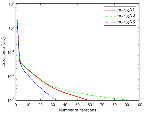
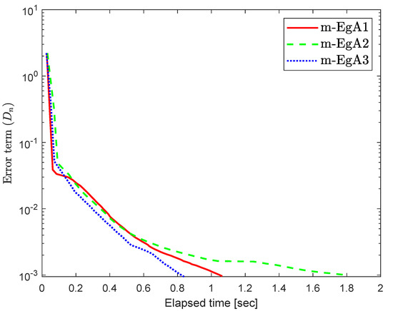
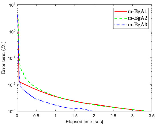
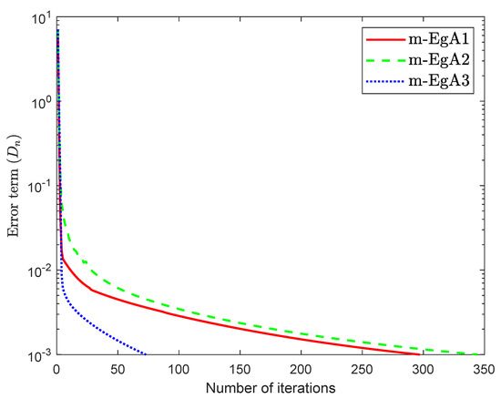
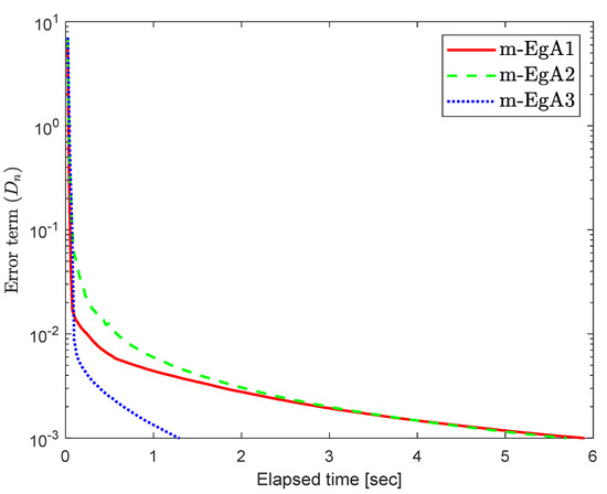
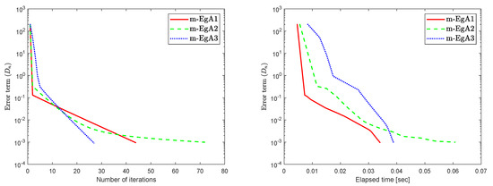
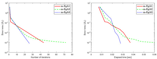
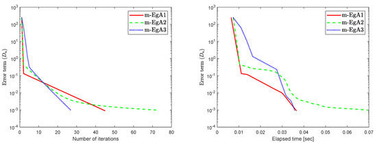
where Q is an $100\times m$ matrix and b is a nonnegative vector in ${\mathbb{R}}^m$. It is clear that F is monotone and Lipschitz continuous with $L=\parallel M\parallel .$ For $q=0$, the solution set of the corresponding variational inequality is $VI(\mathcal{C},F)=\left\{0\right\}$. In this experiment, we take the initial point $u_0=(1,1,\cdots ,1)$ and $D_n=\parallel u_n-v_n\parallel \le TOL={10}^{-3}.$ Moreover, the control parameters ${\zeta }_0=\frac{0.7}{L}$ and $\mu =0.9$ for Algorithm 1 (m-EgA1) in [30]; ${\zeta }_0=\frac{0.7}{L}$, $\mu =0.9$ and ${\beta }_n=\frac{1}{30(k+2)}$ for Algorithm 2 (m-EgA2) in [30]; ${\zeta }_0=\frac{0.7}{L},$$\mu =0.9,$ ${\beta }_n=\frac{1}{n+4}$ and $f\left(u\right)=\frac{u}{2}$ for Algorithm 1 (m-EgA3). The numerical results of all methods have been reported in Figure 1, Figure 2, Figure 3, Figure 4, Figure 5, Figure 6, Figure 7 and Figure 8 and Table 1.

Figure 1. Numerical behaviour of Algorithm 1 compared to Algorithm 1 in [30] and Algorithm 2 in [30] for Example 1, when $m=5$.

Figure 2. Numerical behaviour of Algorithm 1 compared to Algorithm 1 in [30] and Algorithm 2 in [30] for Example 1, when $m=5$.

Figure 3. Numerical behaviour of Algorithm 1 compared to Algorithm 1 in [30] and Algorithm 2 in [30] for Example 1, when $m=10$.

Figure 4. Numerical behaviour of Algorithm 1 compared to Algorithm 1 in [30] and Algorithm 2 in [30] for Example 1, when $m=10$.

Figure 5. Numerical behaviour of Algorithm 1 compared to Algorithm 1 in [30] and Algorithm 2 in [30] for Example 1, when $m=20$.

Figure 6. Numerical behaviour of Algorithm 1 compared to Algorithm 1 in [30] and Algorithm 2 in [30] for Example 1, when $m=20$.

Figure 7. Numerical behaviour of Algorithm 1 compared to Algorithm 1 in [30] and Algorithm 2 in [30] for Example 1, when $m=50$.

Figure 8. Numerical behaviour of Algorithm 1 compared to Algorithm 1 in [30] and Algorithm 2 in [30] for Example 1, when $m=50$.

Table 1. Numerical results numeric values for Figure 1, Figure 2, Figure 3, Figure 4, Figure 5, Figure 6, Figure 7 and Figure 8.

	m-EgA1 [30]		m-EgA2 [30]		m-EgA3
m	Iter.	Time	Iter.	Time	Iter.	Time
5	59	1.0641	92	1.8107	34	0.8386
10	126	2.2007	137	1.9408	73	1.0267
20	204	3.2879	231	3.3654	83	11.9559
50	297	5.8990	344	5.6944	73	1.2942

Example 2.

Assume that $\mathbb{H}=L^2\left([0,1]\right)$ is a Hilbert space with an inner product

$$⟨u,v⟩={\int }_0^{1}u\left(t\right)v\left(t\right)dt,\forall u,v\in \mathbb{H},$$

and the induced norm is

$$\parallel u\parallel =\sqrt{{\int }_0^1{\left|u\left(t\right)\right|}^{2}dt}.$$

Let $\mathcal{C}:=\{u\in L^2\left([0,1]\right):\parallel u\parallel \le 1\}$ be the unit ball and $F:\mathcal{C}\to \mathbb{H}$ is defined by

$$F\left(u\right)\left(t\right)={\int }_0^1\left(u\left(t\right)-H(t,s)f\left(u\right(s\left)\right)\right)ds+g\left(t\right),$$

where

$$H(t,s)=\frac{2ts{e}^{(t+s)}}{e\sqrt{e^2-1}},f\left(u\right)=cos\left(u\right),g\left(t\right)=\frac{2t{e}^t}{e\sqrt{e^2-1}}.$$

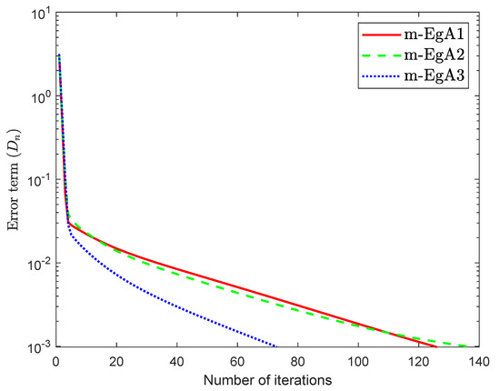
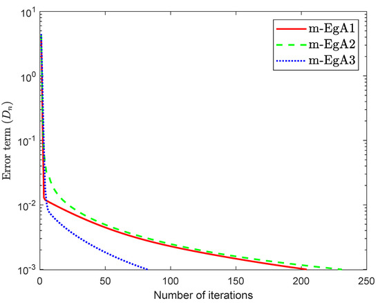
We can see in [41], that F is Lipschitz-continuous with Lipschitz constant $L=2$ and monotone. Figure 9, Figure 10 and Figure 11 and Table 2 show the numerical results by taking different initial values $u_0$ and $ϵ={10}^{-3}.$ In this experiment, we take the different initial points $u_0$ and $D_n=\parallel u_n-v_n\parallel \le TOL={10}^{-3}.$ Moreover, the control parameters ${\zeta }_0=\frac{0.6}{L}$ and $\mu =0.45$ for Algorithm 1 (m-EgA1) in [30]; ${\zeta }_0=\frac{0.6}{L}$, $\mu =0.45$ and ${\beta }_n=\frac{1}{100(k+2)}$ for Algorithm 2 (m-EgA2) in [30]; ${\zeta }_0=\frac{0.6}{L},$$\mu =0.45,$ ${\beta }_n=\frac{1}{n+2}$ and $f\left(u\right)=\frac{u}{3}$ for Algorithm 1 (m-EgA3).

Figure 9. Numerical behaviour of Algorithm 1 compared to Algorithm 1 in [30] and Algorithm 2 in [30] for Example 1, when $u_0=t$.

Figure 10. Numerical behaviour of Algorithm 1 compared to Algorithm 1 in [30] and Algorithm 2 in [30] for Example 1, when $u_0=sin\left(t\right)$.

Figure 11. Numerical behaviour of Algorithm 1 compared to Algorithm 1 in [30] and Algorithm 2 in [30] for Example 1, when $u_0=cos\left(t\right)$.

Table 2. Numerical comparison values for Figure 1, Figure 2, Figure 3, Figure 4, Figure 5, Figure 6, Figure 7 and Figure 8.

	m-EgA1 [30]		m-EgA2 [30]		m-EgA3
${\mathit{u}}_0$	Iter.	Time	Iter.	Time	Iter.	Time
t	44	0.0342	72	0.0609	27	0.0390
$sin\left(t\right)$	44	0.0876	72	0.0569	40	0.0569
$cos\left(t\right)$	45	0.0366	72	0.0358	27	0.0358

Example 3.

Let $F:{\mathbb{R}}^2\to {\mathbb{R}}^2$ is defined by

$$F\left(\begin{array}{c}{u}_1\\ u_2\end{array}\right)=\left(\begin{array}{c}{u}_1+u_2+sin\left(u_1\right)\\ -u_1+u_2+sin\left(u_2\right)\end{array}\right),\forall \left(\begin{array}{c}{u}_1\\ u_2\end{array}\right)\in {\mathbb{R}}^2$$

and $\mathcal{C}$ is taken as

$$\mathcal{C}=\{u={(u_1,u_1)}^T\in {\mathbb{R}}^2:0\le u_i\le 10,i=1,2\}.$$

This problem was proposed in [43], where F is L-Lipschitz continuous with Lipschitz constant $L=\sqrt{10}$ and monotone. In this experiment, we take the different initial points $u_0$ and $D_n=\parallel u_n-v_n\parallel \le TOL.$ Moreover, the control parameters ${\zeta }_0=\frac{0.7}{L}$ and $\mu =0.50$ for Algorithm 1 (m-EgA1) in [30]; ${\zeta }_0=\frac{0.7}{L}$, $\mu =0.50$ and ${\beta }_n=\frac{1}{100(n+2)}$ for Algorithm 2 (m-EgA2) in [30]; ${\zeta }_0=\frac{0.7}{L},$$\mu =0.50,$${\beta }_n=\frac{1}{100(n+2)}$ and $f\left(u\right)=\frac{u}{4}$ for Algorithm 1 (m-EgA3). Table 3 reports the numerical results by using different tolerance and initial points.

Table 3. Numerical behaviour of Algorithm 1 compared to Algorithm 1 in [30] and Algorithm 2 in [30] for Example 3 by using different initial points $u_0$.

	TOL	0.01	0.001	0.0001	0.00001	0.01	0.001	0.0001	0.00001
	${\mathit{u}}_0$	Iter.	Iter.	Iter.	Iter.	Time	Time	Time	Time
Algorithm 1 in [30]
	${[10,20]}^T$	29	41	83	277	0.4668	0.6234	1.5395	3.0415
	${[-10,-10]}^T$	45	57	117	345	0.9234	1.1440	1.7387	3.4382
	${[10,20]}^T$	59	71	143	389	1.0806	1.4264	1.8271	3.9269
Algorithm 2 in [30]
	${[10,20]}^T$	31	42	87	290	0.4743	0.5981	1.4921	3.2051
	${[-10,-10]}^T$	45	61	115	360	0.8976	1.2081	1.5891	3.7891
	${[10,20]}^T$	69	73	151	407	1.2711	1.3910	2.0810	4.1981
Algorithm 1
	${[10,20]}^T$	19	26	49	119	0.2391	0.3871	0.7716	1.6781
	${[-10,-10]}^T$	25	39	64	123	0.2991	0.5192	0.9981	1.7021
	${[10,20]}^T$	31	45	73	189	0.3018	0.7610	1.1012	2.4071

References

- Stampacchia, G. Formes bilinéaires coercitives sur les ensembles convexes. Comptes Rendus Hebd. Des Seances De L Acad. Des Sci. 1964, 258, 4413. [Google Scholar]
- Konnov, I.V. On systems of variational inequalities. Russ. Math. C/C-Izv.-Vyss. Uchebnye Zaved. Mat. 1997, 41, 77–86. [Google Scholar]
- Kassay, G.; Kolumbán, J.; Páles, Z. On Nash stationary points. Publ. Math. 1999, 54, 267–279. [Google Scholar]
- Kassay, G.; Kolumbán, J.; Páles, Z. Factorization of Minty and Stampacchia variational inequality systems. Eur. J. Oper. Res. 2002, 143, 377–389. [Google Scholar] [CrossRef]
- Kinderlehrer, D.; Stampacchia, G. An Introduction to Variational Inequalities and Their Applications; Society for Industrial and Applied Mathematics: Philadelphia, PA, USA, 2000. [Google Scholar] [CrossRef]
- Konnov, I. Equilibrium Models and Variational Inequalities; Elsevier: Amsterdam, The Netherlands, 2007; Volume 210. [Google Scholar]
- Takahashi, W. Introduction to Nonlinear and Convex Analysis; Yokohama Publishers: Yokohama, Japan, 2009. [Google Scholar]
- Korpelevich, G. The extragradient method for finding saddle points and other problems. Matecon 1976, 12, 747–756. [Google Scholar]
- Noor, M.A. Some iterative methods for nonconvex variational inequalities. Comput. Math. Model. 2010, 21, 97–108. [Google Scholar] [CrossRef]
- Censor, Y.; Gibali, A.; Reich, S. The subgradient extragradient method for solving variational inequalities in Hilbert space. J. Optim. Theory Appl. 2010, 148, 318–335. [Google Scholar] [CrossRef]
- Censor, Y.; Gibali, A.; Reich, S. Extensions of Korpelevich’s extragradient method for the variational inequality problem in Euclidean space. Optimization 2012, 61, 1119–1132. [Google Scholar] [CrossRef]
- Malitsky, Y.V.; Semenov, V.V. An Extragradient Algorithm for Monotone Variational Inequalities. Cybern. Syst. Anal. 2014, 50, 271–277. [Google Scholar] [CrossRef]
- Tseng, P. A Modified Forward-Backward Splitting Method for Maximal Monotone Mappings. SIAM J. Control Optim. 2000, 38, 431–446. [Google Scholar] [CrossRef]
- Moudafi, A. Viscosity Approximation Methods for Fixed-Points Problems. J. Math. Anal. Appl. 2000, 241, 46–55. [Google Scholar] [CrossRef]
- Zhang, L.; Fang, C.; Chen, S. An inertial subgradient-type method for solving single-valued variational inequalities and fixed point problems. Numer. Algorithms 2018, 79, 941–956. [Google Scholar] [CrossRef]
- Iusem, A.N.; Svaiter, B.F. A variant of korpelevich’s method for variational inequalities with a new search strategy. Optimization 1997, 42, 309–321. [Google Scholar] [CrossRef]
- Thong, D.V.; Hieu, D.V. Modified subgradient extragradient method for variational inequality problems. Numer. Algorithms 2017, 79, 597–610. [Google Scholar] [CrossRef]
- Thong, D.V.; Hieu, D.V. Weak and strong convergence theorems for variational inequality problems. Numer. Algorithms 2017, 78, 1045–1060. [Google Scholar] [CrossRef]
- Marino, G.; Scardamaglia, B.; Karapinar, E. Strong convergence theorem for strict pseudo-contractions in Hilbert spaces. J. Inequal. Appl. 2016, 2016. [Google Scholar] [CrossRef]
- Ur Rehman, H.; Kumam, P.; Cho, Y.J.; Yordsorn, P. Weak convergence of explicit extragradient algorithms for solving equilibirum problems. J. Inequal. Appl. 2019, 2019. [Google Scholar] [CrossRef]
- Ur Rehman, H.; Kumam, P.; Je Cho, Y.; Suleiman, Y.I.; Kumam, W. Modified Popov’s explicit iterative algorithms for solving pseudomonotone equilibrium problems. Optim. Methods Softw. 2020, 1–32. [Google Scholar] [CrossRef]
- Ur Rehman, H.; Kumam, P.; Abubakar, A.B.; Cho, Y.J. The extragradient algorithm with inertial effects extended to equilibrium problems. Comput. Appl. Math. 2020, 39. [Google Scholar] [CrossRef]
- Ur Rehman, H.; Kumam, P.; Kumam, W.; Shutaywi, M.; Jirakitpuwapat, W. The inertial sub-gradient extra-gradient method for a class of pseudo-monotone equilibrium problems. Symmetry 2020, 12, 463. [Google Scholar] [CrossRef]
- Ur Rehman, H.; Kumam, P.; Argyros, I.K.; Deebani, W.; Kumam, W. Inertial extra-gradient method for solving a family of strongly pseudomonotone equilibrium problems in real Hilbert spaces with application in variational inequality problem. Symmetry 2020, 12, 503. [Google Scholar] [CrossRef]
- Ur Rehman, H.; Kumam, P.; Argyros, I.K.; Alreshidi, N.A.; Kumam, W.; Jirakitpuwapat, W. A self-adaptive extra-gradient methods for a family of pseudomonotone equilibrium programming with application in different classes of variational inequality problems. Symmetry 2020, 12, 523. [Google Scholar] [CrossRef]
- Ur Rehman, H.; Kumam, P.; Argyros, I.K.; Shutaywi, M.; Shah, Z. Optimization based methods for solving the equilibrium problems with applications in variational inequality problems and solution of Nash equilibrium models. Mathematics 2020, 8, 822. [Google Scholar] [CrossRef]
- Ur Rehman, H.; Kumam, P.; Shutaywi, M.; Alreshidi, N.A.; Kumam, W. Inertial optimization based two-step methods for solving equilibrium problems with applications in variational inequality problems and growth control equilibrium models. Energies 2020, 13, 3292. [Google Scholar] [CrossRef]
- Rehman, H.U.; Kumam, P.; Dong, Q.L.; Peng, Y.; Deebani, W. A new Popov’s subgradient extragradient method for two classes of equilibrium programming in a real Hilbert space. Optimization 2020, 1–36. [Google Scholar] [CrossRef]
- Antipin, A.S. On a method for convex programs using a symmetrical modification of the Lagrange function. Ekon. I Mat. Metod. 1976, 12, 1164–1173. [Google Scholar]
- Yang, J.; Liu, H.; Liu, Z. Modified subgradient extragradient algorithms for solving monotone variational inequalities. Optimization 2018, 67, 2247–2258. [Google Scholar] [CrossRef]
- Kraikaew, R.; Saejung, S. Strong Convergence of the Halpern Subgradient Extragradient Method for Solving Variational Inequalities in Hilbert Spaces. J. Optim. Theory Appl. 2013, 163, 399–412. [Google Scholar] [CrossRef]
- Heinz, H.; Bauschke, P.L.C. Convex Analysis and Monotone Operator Theory in Hilbert Spaces, 2nd ed.; CMS Books in Mathematics; Springer International Publishing: New York, NY, USA, 2017. [Google Scholar]
- Kreyszig, E. Introductory Functional Analysis with Applications, 1st ed.; Wiley Classics Library: Hoboken, NJ, USA, 1989. [Google Scholar]
- Xu, H.K. Another control condition in an iterative method for nonexpansive mappings. Bull. Aust. Math. Soc. 2002, 65, 109–113. [Google Scholar] [CrossRef]
- Maingé, P.E. Strong Convergence of Projected Subgradient Methods for Nonsmooth and Nonstrictly Convex Minimization. Set-Valued Anal. 2008, 16, 899–912. [Google Scholar] [CrossRef]
- Takahashi, W. Nonlinear Functional Analysis; Yokohama Publisher: Yokohama, Japan, 2000. [Google Scholar]
- Liu, Z.; Zeng, S.; Motreanu, D. Evolutionary problems driven by variational inequalities. J. Differ. Equ. 2016, 260, 6787–6799. [Google Scholar] [CrossRef]
- Liu, Z.; Migórski, S.; Zeng, S. Partial differential variational inequalities involving nonlocal boundary conditions in Banach spaces. J. Differ. Equ. 2017, 263, 3989–4006. [Google Scholar] [CrossRef]
- Harker, P.T.; Pang, J.S. for the Linear Complementarity Problem. Comput. Solut. Nonlinear Syst. Equ. 1990, 26, 265. [Google Scholar]
- Solodov, M.V.; Svaiter, B.F. A New Projection Method for Variational Inequality Problems. SIAM J. Control Optim. 1999, 37, 765–776. [Google Scholar] [CrossRef]
- Van Hieu, D.; Anh, P.K.; Muu, L.D. Modified hybrid projection methods for finding common solutions to variational inequality problems. Comput. Optim. Appl. 2016, 66, 75–96. [Google Scholar] [CrossRef]
- Dong, Q.L.; Cho, Y.J.; Zhong, L.L.; Rassias, T.M. Inertial projection and contraction algorithms for variational inequalities. J. Glob. Optim. 2017, 70, 687–704. [Google Scholar] [CrossRef]
- Dong, Q.L.; Lu, Y.Y.; Yang, J. The extragradient algorithm with inertial effects for solving the variational inequality. Optimization 2016, 65, 2217–2226. [Google Scholar] [CrossRef]
Publisher’s Note: MDPI stays neutral with regard to jurisdictional claims in published maps and institutional affiliations. |
© 2020 by the authors. Licensee MDPI, Basel, Switzerland. This article is an open access article distributed under the terms and conditions of the Creative Commons Attribution (CC BY) license (http://creativecommons.org/licenses/by/4.0/).