Abstract
In this study, a novel digital compound compensation method is proposed to compensate for the hysteresis nonlinearity and the drift disturbance of a piezoelectric nanopositioning system with a large range. The overall hysteresis behaviors can be divided into the static amplitude-dependent behavior and the dynamic rate-dependent behavior, where the static hysteresis is compensated for by a novel discrete feedforward controller, while the dynamic hysteresis and the drift disturbance are compensated for by a novel discrete composite feedback controller composed of a drift observer-based state feedback controller and a repetitive learning controller. Compared with traditional control strategies, the proposed compound control strategy, including feedforward and feedback components, can eliminate system errors more effectively when tracking large range signals with obvious hysteresis. Moreover, the proposed online drift observer is superior over a traditional offline drift compensator both in response speed and compensation accuracy. Sufficient simulation tests and convincing tracking experiments, with large range periodic signals up to 90 m, are carried out. And comparisons with the two classical control algorithms are performed. The tracking results show that the mean absolute error of the proposed control method is minor compared with the other two algorithms, which validates that the proposed strategy can efficiently compensate for the hysteresis nonlinearity and the drift disturbance.
1. Introduction
Piezoelectric driven nanopositioning systems play important roles in ultra precise instruments such as atomic force microscopes [1,2,3], scanning tunneling microscopes, and ultra-precision machine tools, etc. Piezoelectric actuators (PEAs) have become the first choice in the nanopositoning field for its outstanding advantages of ultra high resolution, fast response, high bandwidth, large driven force, and high stiffness [4]. The resolution of piezoelectric actuators can reach a few tenths of nanometer accuracy or be even more precise. When tracking nanometer level step signals, their response time can be as small as several microseconds, or even smaller. The bandwidth of some piezoelectric actuators can reach several thousands hertz. Although piezoelectric actuators possess a number of advantages, as listed above, they have to deal with some typical drawbacks as well, mainly including hysteresis, creep, drift, and so on, wherein hysteresis and drift are the two apparent features, especially when tracking large range and time varying signals, which need to be carefully tackled to achieve satisfactory performance.
Hysteresis, behaving as significant nonlinearity between input voltage and output displacements, is the main reason of positioning error. In fact, the hysteresis effect of the PEA turns even worse as the travel range becomes larger. Specifically, the hysteresis can be divided into two categories: static hysteresis and dynamic hysteresis. Static hysteresis is caused by the inertial physics of piezoelectric actuators themselves and is mainly related to the travel range, while dynamic hysteresis is stimulated by the input signal and mainly relates with the frequency of the input signal, which can be depicted by the frequency response or the state space representation. To deal with the hysteresis nonlinearity, many researches have been conducted and various effective strategies with meaningful results have been reported [5,6,7]. Some effective mathematical models have been constructed to precisely describe the static hysteresis for the error compensation. For example, Duhem model is developed for the hysteresis description, which is effective to describe the static hysteresis behaviors of piezoelectric actuators [8]. The backlash-like model and Bouc–Wen model are developed to describe and compensate for the static hysteresis, which simplify the mathematical representation and decrease the depiction error [9,10,11]. Besides, operator-based models, such as the Preisach model and the Prandtl–Ishlinskii model, are also proposed to implement compensation for hysteresis [12]. Recently, neural network (NN), T-S fuzzy system and deep learning technology have been adopted in the PEA hysteresis modeling through offline data training, and some effective results have been reported [13,14,15]. These modeling and compensation methods mentioned above, though effective in some cases, cannot usually achieve satisfactory performance for a large range piezoelectric actuator. That is, through decades of efforts, although much improvement has been achieved for hysteresis modeling and compensation [16], it is still a fairly open problem facing many challenges.
Drift is another factor decreasing the positioning accuracy and leading to measurement errors of the PEA in practical applications [17]. The thermal drift drives piezoelectric actuators to gradually deviate from the given set-point. Different strategies are proposed to model the drift, based on which, various compensation methods are designed to reduce the errors caused by the drift disturbance. It is noted that most of the reported methods mainly turn to offline modeling and compensation to deal with the thermal drift, whose performance cannot be guaranteed when the environment changes sharply or the initial drift offset point alters for some reasons. Therefore, effective drift estimation and elimination via a real-time method is a very promising and challenging direction [18], which needs to be further investigated.
Since the aforementioned drawbacks notably affect the PEA tracking performance, designing effective real-time feedforward/feedback controllers to decrease tracking errors becomes one of the most important issues for a PEA positioning system. As the nonlinear control technology and the intelligent control technology have developed rapidly in recent years [19,20,21], many advanced control technologies are implemented to compensate for the nonlinearity and disturbances in piezoelectric actuators [22,23,24,25]. Until now, many researchers have engaged in the PEA nanopositioning control with a number of different strategies and significant results have recently been reported. For example, a feedforward component is combined with some feedback control strategies to achieve precise tracking of piezoelectric actuators in Ref. [26]. In periodical signal tracking, repetitive control is considered as an efficient closed-loop compensation solution, and in Ref. [27], a novel repetitive control algorithm is designed to deal with the hysteresis nonlinearity of piezoelectric actuators. Besides, repetitive learning control has been validated to be able to obtain satisfactory results in dealing with periodical disturbance, and in Ref. [28], an adaptive repetitive learning control method is designed to handle the periodical disturbances on the piezo-driven cantilever. Observer-based control methods are also effective compensation solutions by combining the online observers with nonlinear control algorithms. In Ref. [29], a novel high-performance control scheme with a hysteresis compensator and a disturbance observer is designed for the high-precision motion control of a nanopositioning stage driven by a piezoelectric actuator, and the experimental results demonstrate the effectiveness of the proposed method. Recently, the sliding mode control method [30] has been widely explored to stabilize the piezoelectric nanopositioning systems, and a variety of advanced sliding mode control strategies have been designed to the meet different requirements for various practical systems. In Ref. [31], a perturbation estimation-based sliding mode control method combined with an inverse Bouc-Wen model based hysteresis compensator is designed, and the asymptotical stability of the closed-loop system is obtained via Lyapunov-based analysis. The combined control strategy can compensate for the hysteresis nonlinearity and estimate the disturbance online, thus improving the robustness and the tracking accuracy of the system. The traditional sliding mode control method is limited in practical system application for the chattering phenomenon. Due to this reason, a number of continuous sliding mode control strategies are proposed to handle the chattering [32]. In recent years, the neural network (NN) based control algorithm has become a popular tool to deal with various uncertainties in the PEA component, which takes advantages of real-time learning for all kinds of uncertainties, yet the loop calculation becomes a burden when the knots of network increase to a certain extent [33].
In this paper, a novel discrete compound control strategy is proposed to deal with the hysteresis nonlinearity and the drift disturbance of a large range piezoelectric nanopositioning system. The static amplitude-dependent hysteresis and the dynamic rate-dependent hysteresis are compensated for by a feedforward controller and a feedback controller, respectively. Specifically, an online discrete observer is designed to provide real-time correction for the disturbance, and a Lyapunov-based repetitive learning controller is employed to eliminate periodic unmodeled dynamics during the tracking process. The contributions of this paper are summarized as follows:
- A novel discrete compound control strategy, composed of a feedforward controller and a composite feedback controller, is proposed to guarantee the tracking performance of the large range PEA nanopositioning system;
- An efficient online discrete nonlinear observer is designed to implement a real-time estimation for the disturbance;
- A novel observer-based repetitive learning feedback control algorithm is designed, and the discrete Lyapunov-based stability analysis is provided to prove that the tracking error is globally uniformly ultimately bounded.
The rest of this paper is organized as follows. In Section 2, a system identification algorithm, including dynamic model parameters identification and static hysteresis calibration, is proposed. In Section 3, the system control issue is explicitly formulated and the discrete control strategy is proposed. In Section 4, the stability of the discrete closed-loop system is provided via the Lyapunov-based thoery. In Section 5, simulation tests are performed to illustrate the effectiveness of the proposed strategy. In Section 6, simulations and experiments are carried out, and comparative experiments with two other traditional control methods are performed to test the tracking accuracy of the proposed control method. Finally, the conclusions are presented in Section 7.
2. System Modeling and Parameter Identification
This section introduces the dynamic model of the piezoelectric actuators and the identification of the system parameters and the static hysteresis, which contains three subsections. The first one is dynamic system modeling, where the dynamic model of piezoelectric actuators is built. The second subsection is static hysteresis calibration, where an effective numerical calibration method is proposed to approximate the discrete nonlinear function of static hysteresis. The third subsection is modeling accuracy validation, where the accuracy of the proposed model is tested.
2.1. Dynamic Modeling
The spring-mass-damping dynamic model of the piezoelectric actuators is presented as follows:
where t denotes the time variable, and , , denote the mass, the damping coefficient, and the stiffness in the spring-mass-damping model, respectively, b is the input coefficient, and , represent the static hysteresis and the system disturbance.
In the piezoelectric actuators period signal tracking issues, the disturbance is mainly made up of two parts, which can be expressed as follows:
where is the desired periodical signal, is a slowly varying signal, and is the periodical signal.
Considering the hardware physical state, a reasonable assumption is presented as follows:
Assumption 1.
All disturbances and their derivatives, such as , , , , , and in the piezoelectric actuators, are bounded.
To facilitate the following analysis, without loss of generality, let and the Equation (1) be expressed as follows:
To calibrate the coefficients , , b, the swept-sine signals are put into the piezoelectric actuators, and the frequency responses of the inputs and outputs are obtained via the experiment. The transfer function of the piezoelectric actuators is obtained via the System Identification Toolbox of Matlab, which is presented as follows:
where s is the Laplace operator, the input signal is the voltage on the piezoelectric actuators platform, and the output signal is the voltage of the capacitive displacement sensor, where stands for 10 m. According to transfer function in (4), the dynamic parameters in (3) are identified as , , , respectively.
2.2. Static Hysteresis Calibration
Static hysteresis is caused by the inertial electromagnetic properties of the piezoelectric actuators, which is irrelevant with the scanning frequency, yet closely relevant with the amplitude of the input signal. The static hysteresis nonlinearity becomes severe as the amplitude of the input signal increases. Thus, aiming at tracking for the large range periodic signals, a novel and efficient discrete static hysteresis calibration method is proposed, fully taking advantage of the properties of static hysteresis.
First, a low scanning frequency sinusoid signal is input into the piezoelectric actuators platform, in which the dynamics of the piezoelectric actuators is small enough to be ignored and the overall hysteresis is regarded as only including the static hysteresis. As shown in Figure 1, for low frequency scanning, the system dynamics is neglectable, and the static hysteresis loops of (blue solid line) and (red dotted line) closely coincide with each other. As shown in Figure 2, from to , the hysteresis loop expands rapidly with the increase of the scanning frequency, comparing with that of and , where the increased part of the hysteresis loop is determined by the dynamic characteristics. To facilitate the subsequent calculation, the hysteresis loop of is selected to calculate the static hysteresis function, whose discrete equation is expressed as follows:
where is the static hysteresis function in , is the output of the PEA platform, is the sinusoid input signal, is the discrete time, , are amplitudes of the open-loop input and output signals respectively, and and are data sequences in the discrete form, which can be obtained in the experiment.
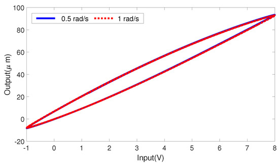
Figure 1.
Hysteresis loops with sinusoid signal inputs of and .
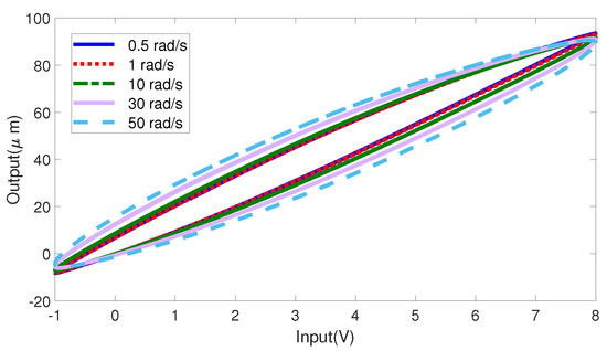
Figure 2.
Hysteresis loops with five different sinusoid signal inputs of angular velocities from to .
The discrete equation of the static hysteresis function in is expressed as follows:
where is the integral angular velocity, is the signal period in , is the sampling time interval. According to (5) and (6), the periodic static hysteresis function of any integral angular velocity can be calculated with input/output signals of the same amplitude. Selecting the sample time as , the static hysteresis functions of the input sinusoid signals with the 90 m travel range, with four different angular velocities as , , , , are shown in Figure 3.
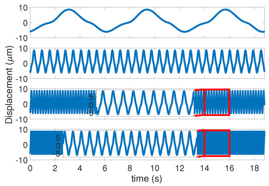
Figure 3.
Periodic static hysteresis functions with angular velocities of , , , from top to bottom, respectively.
According to the static hysteresis function in (6), the discrete form of the static hysteresis term in system (3) is expressed as follows:
where b is the coefficient in (3), , are amplitudes of the open-loop input and output signals, respectively. To facilitate the model validation in the following subsection, the discrete form of the system in Ref. (3) is presented as follows:
where the delta operator is defined as follows:
with being the sampling time, and , being the displacement signals in two adjacent sampling moments.
2.3. Modeling Accuracy Validation
In this subsection, the accuracy of the piezoelectric actuators model, including both the obtained dynamic model and the static hysteresis calibration illustrated in the previous two subsections, is validated through experiments.
To validate the effectiveness of the piezoelectric actuators modeling method proposed in the first two subsections, sinusoid signals with a large travel range up to 90 m and angular velocities of and , respectively, which can stimulate the hysteresis characteristics to a relatively high level, are input into the real piezoelectric actuators platform and the constructed mathematical model, respectively. The sampling period is set as . The obtained results are shown in Figure 4, from which it is clear that the overall hysteresis loops (the red one is generated by the piezoelectric actuators platform and the blue one is generated by the mathematical model), including the static part and the dynamic part, closely coincide with each other. The results demonstrate that the mathematical model well describes the hysteresis characteristics, even for the large range input signals with high angular velocity. As will be illustrated subsequently, the unmodeled uncertainty and the thermal drift disturbance can be compensated by the Lyapunov-based nonlinear feedback control method designed in the following sections.
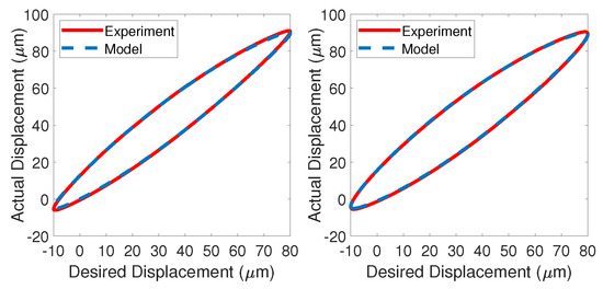
Figure 4.
Hysteresis loops generated by the experiment and the model ( with the left subfigure and with the right subfigure).
Remark 1.
In this paper, periodical signals are labeled by angular velocities (rad/s) instead of frequencies (Hz), which can be conveniently converted with each other. For example, signals with angular velocities of 10 rad/s, 30 rad/s and 50 rad/s are corresponding to frequencies of 1.59 Hz, 4.77 Hz and 7.96 Hz.
3. Closed-Loop System Control Method Design
This section presented the system tracking problem formulation and nonlinear controller design. An effective discrete disturbance observer is constructed and a discrete nonlinear feedback control strategy, combined with the Lyapunov-based repetitive learning control technology, is proposed to compensate for the tracking error.
3.1. Tracking Error System Formulation
The tracking error is defined as follows:
where is the piezoelectric actuators system tracking error, is the displacement signal, and is the reference signal in the tracking task. With the delta operator in (9), the first order and second order derivatives of in the discrete form are expressed as follows:
The constructed model of the piezoelectric actuators (3) is substituted into (12), and the following error dynamic system is presented:
A first order linear filter auxiliary signal and its derivative in discrete form are defined as follows:
where is the parameter.
Then, (13) is substituted into (15), and the open loop error system of the piezoelectric actuators is presented as follows:
With all signals discretized in (16), the discrete compound controller is proposed in the next subsection.
3.2. Controller Design
The discrete compound controller is proposed as follows:
where is the displacement signal of the piezoelectric actuators, is the reference signal in the tracking task, , with the updated law by the discrete nonlinear observer, is the estimation of the drift disturbance, , updated by the repetitive learning control law, is the estimation of the periodical unmodeled uncertainty, is the static hysteresis function calibrated in (6), b, , are identified system parameters, and , , are the control gains.
As shown in Figure 5, to facilitate the analysis and illustrate the work principle more clearly, the discrete compound control strategy is divided into three control layers. In the first layer, the static amplitude-dependent hysteresis is compensated by the feedforward sub-controller and the feedback controller, respectively. In the second layer, the dynamic rate-dependent hysteresis is compensated by the system state feedback sub-controller, and specifically, an online discrete observer is designed to provide real time correction for the disturbance. In the third layer, the Lyapunov-based repetitive learning sub-controller is employed to eliminate periodic unmodeled dynamics during the tracking process. As illustrated in Figure 5, the compound controller is expressed in a form of three sub-controllers, as follows:
where is the observer-based state feedback controller, is the feedforward controller, and is the repetitive learning controller.
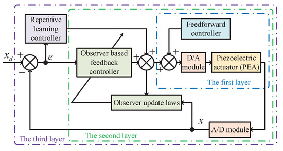
Figure 5.
Control system diagram.
Then, inspired by Ref. [34], the discrete disturbance observer is designed as follows:
where is the estimation of the thermal drift disturbance, z is an auxiliary variable, and is an observer gain.
Taking the time difference on both sides of (23), the following equation is obtained:
which, by substituting (23), can be further rewritten into the following form:
Furthermore, the following discrete difference equation is obtained by substituting the open-loop error system (16) into (25):
where .
According to Assumption 1, is bounded by a positive constant :
Thus, utilizing (26), the following inequality is obtained:
whose solution can be expressed as follows:
implying that is bounded.
Meanwhile, based on (26), the following expression is obtained:
where is the sampling interval. According to (2), the disturbance is mainly made up of two parts as:
where is a slowly varying signal, and is the periodical signal.
By substituting (31) into (30), the observer error can be then calculated as follows:
where is presented as:
According to Assumption 1 and (29), both and are bounded. Then, from (32), it is seen that is bounded.
The periodical error can be estimated by the following repetitive learning algorithm. The repetitive learning law is designed as follows:
where is the period of , is a control gain, and is the saturation function defined as follows:
4. Discrete Closed-Loop System Stability Analysis
The globally uniformly ultimately bounded stability of the discrete closed-loop system is derived through the Lyapunov-based method. The main stability theorem is presented as follows.
Theorem 1.
Proof.
The closed-loop error system is obtained by substituting the control law (17) into the open-loop error system (16), which is presented as follows:
with being the estimation errors of , explicitly defined as:
According to the closed-loop error system, the following Lyapunov function candidate is constructed:
To facilitate the mathematic description in the next step, the following auxiliary signal is defined:
then, can be rewritten into the following form:
The difference equation of is obtained via the delta operator as follows:
To facilitate the description, the following substitution is introduced:
With the above substitution, is presented as follows:
Then, noting the following fact [35]:
is transformed as:
Let , then the following inequality is obtained:
To facilitate the description, the following substitution is introduced:
With and bounded, to facilitate the analysis, let be the upper bound of and let . With properly selecting parameters, and can be ensured. Then, (55) can be rewritten into the following form:
The solution of the above differential inequality is expressed as follows:
According to the above analysis, is globally uniformly ultimately bounded (GUUB). Thus, according to the property of the first order linear filter, when is a globally uniformly ultimately bounded (GUUB), the system tracking error is globally uniformly ultimately bounded (GUUB). □
5. Simulation Analysis
The tracking accuracy of the control method poposed in this paper is tested under a MATLAB/SIMULINK environment. To validate the performance of the proposed strategy, large range periodic signal tracking simulations are carried out and the contrasts with two traditional control methods are carried out. In these simulations, the sample period of the control system is .
The dynamic model of the piezoelectric actuators for simulation is presented as follows:
where , , , is calculated by (6) using the off-line experiment data, the time slowly varying signal with a large initial step, namely is selected to simulate the thermal drift. In the nominal model during the simulation, error parameter is adopted to simulate the unmodeled uncertainty as in (60).
The tracking performance of the sinusoid signal in with a rip length of m is presented in Figure 6. The top subfigure presents the output displacement of the system in contrast with the reference, which reveals that, with a large travel range and relatively high speed, the proposed control strategy can compensate for the nonlinearity, disturbances, and uncertainties to ensure high accuracy tracking. The middle subfigure illustrates that the tracking error converges to a very small neighborhood of zero. The oscillating actions in the starting transient interval are caused by the large initial step of thermal drift. The mean absolute error (MAE) of the control method in is 0.0054 m, which is neglectable when compared with the trip length. The bottom subfigure is the control input, which is smooth and effective.
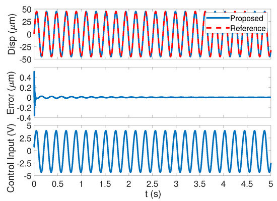
Figure 6.
Simulation results of the sinusoid signal tracking via the proposed control algorithm ().
To further illustrate the advantage of this strategy, comparisons with other two nonlinear control technologies in tracking large range periodic signals are carried out. One is the exact model knowledge (EMK) based feedback control, and the other is the observer-based feedback control. The discrete EMK controller is expressed as follows:
which can exactly compensate for the nonlinearity in the identified model, but is not able to handle the unmodeled dynamics and disturbances. The discrete observer-based controller is presented as follows:
which can estimate the thermal drift disturbances in real-time but the performance is not satisfactory in compensating for unmodeled uncertainties. The system parameters in (61) and (62) are obtained via using the System Identification Toolbox of Matlab, which are the same as the parameters of the dynamic model in (60). Besides, the particle swarm optimization (PSO) method in [31] is also very suitable for the parameter identification of Equations (61) and (62).
The performance comparisons of the three control strategies are presented in Figure 7 and Figure 8. As shown in Figure 7, the sinusoid signal in with m range is tracked via three controllers. The proposed control strategy overwhelms the other two methods in tracking accuracy. The tracking error of the EMK method is the largest among the three methods as a result of drift and unmodeled dynamics. The tracking error of the observer-based method is close to but still not as precise as the proposed method as a result of unmodeled dynamics, which is compensated by the repetitive learning technology in the latter method. The tracking performance comparisons with the reference signal in are shown in Figure 8, whose conclusion is similar as that of Figure 7. Moreover, the proposed method provides much more precise tracking results than the observer-based method in higher speed tracking. For the tracking task with the reference signal in , the mean absolute error (MAE) of the control methods in are m and m by the proposed method and the observer-based method, respectively, which reveals that the error of the observer-based method is 2.75 times of that of the proposed method. For the tracking task with the reference signal in , the mean absolute error (MAE) of the control methods in are m and m by the proposed and the observer-based method, respectively, which reveals that the error of the observer-based method is 3.22 times of that of the proposed method. Through the error analysis above, the ratio of the tracking error with the observer-based method to that with the proposed method increases as the tracking angular velocity rises, which further demonstrates the high performance of the proposed method, especially when tracking relatively high speed signals.
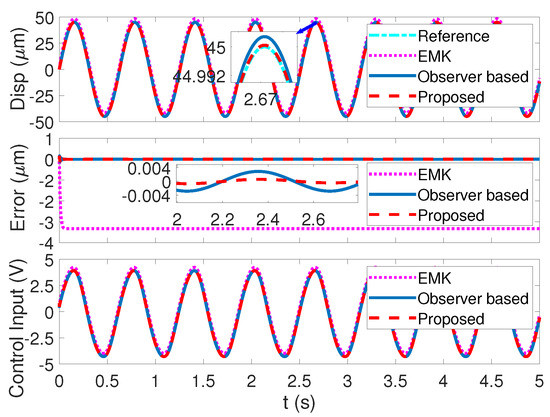
Figure 7.
Simulation results of the three control methods ().
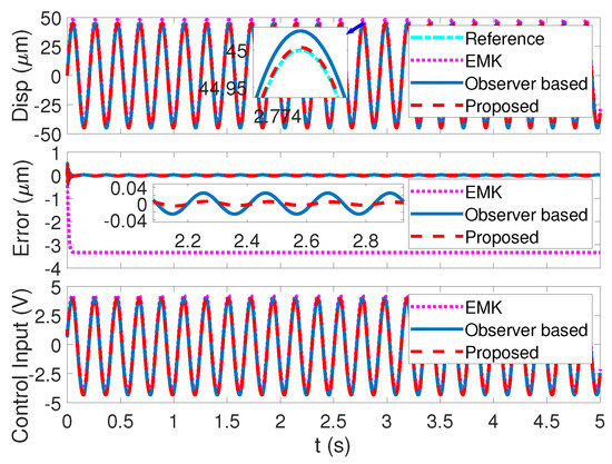
Figure 8.
Simulation results of the three control methods ().
6. Hardware Experiment
In this section, hardware experiments are carried out to validate the tracking performance of the proposed method. The section is divided into two subsections, namely experiment setup and experiment result analysis. The first subsection illustrates the experiment environment for the real-time control system. The second subsection presents the main experiment results, including tracking results for various angular velocities and comparisons with different control strategies.
6.1. Experiment Setup
As presented in Figure 9, experiments in this paper are conducted on the piezoelectric actuators platform (P-517.3CD, Physik Instrumente) installed on a self-made cross-scale atomic force microscope. The mass of the sample platform loaded on PEA is about . The piezoelectric actuators platform is linked with the voltage amplifier (E-505, Physik Instrumente), and the range of the input voltages in the voltage amplifier are from to and the range of the output voltages are from to . The capacitive displacement sensors are embedded in the piezoelectric actuators platform with interfaces in the E-505 voltage amplifier. The E-505 voltage amplifier is linked with the PCI-1716 data acquisition card (Advantech) embeded in the computer. The computer receives the data from the PCI card in real-time and then processes via the nonlinear control algorithm with the toolbox of real-time windows target in MATLAB/SIMULINK, where the discrete control strategies are programmed and performed. The sampling period of the hardware experiment platform is .
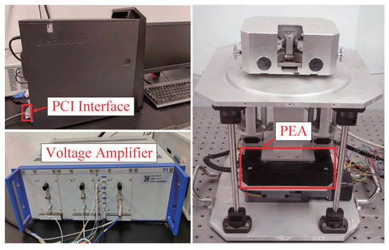
Figure 9.
Experiment setup.
6.2. Experiment Results Analysis
In this subsection, the tracking accuracy of the control method in this paper for different angular velocities is tested on the experiment platform and the comparisons with the control strategies in (61) and (62) are conducted. The control parameters of the three controllers are presented in Table 1.

Table 1.
The control parameters of the three controllers.
The tracking results of the sinusoid reference signals in , , with the trip length of m are presented in Figure 10, Figure 11 and Figure 12. The top subfigures of Figure 10, Figure 11 and Figure 12 are the piezoelectric actuators displacements of the system and the references trajectory, which reveal that, in large travel range and relatively high speed, the control method proposed in this paper can compensate for the nonlinearity and disturbances to guarantee the tracking task in high accuracy. The middle subfigures of Figure 10, Figure 11 and Figure 12 illustrate that the closed-loop system errors stabilize in a very small neighborhood of zero, which corresponds to the stability theorem in Section 4. It can be seen from the results that, since the convergence result of the closed-loop system is GUUB, the tracking error converges to a small neighborhood of zero displacement and cannot completely converge to zero displacement. The mean absolute error (MAE) of the control methods in are m, m and m in , and , respectively, which are , and of the m trip length, respectively. The tracking error increases when the signal angular velocity speeds up.
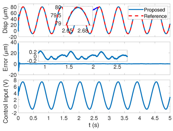
Figure 10.
Experimental results of the sinusoid signal via the proposed algorithm ().
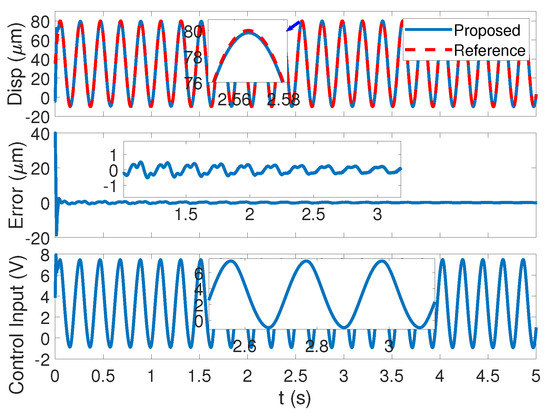
Figure 11.
Experimental results of the sinusoid signal via the proposed algorithm ().
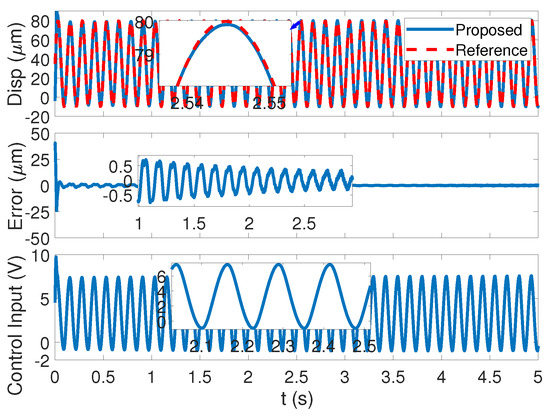
Figure 12.
Experimental results of the sinusoid signal via the proposed algorithm ().
To further analyze the performance of the proposed strategy, comparisons with the EMK control strategy in (61) and the observer-based state feedback control strategy in (62) are made for tracking large range periodic signals with different angular velocities.
The tracking accuracy comparisons with the two other nonlinear control technologies in the piezoelectric actuators platform are presented in Figure 13, Figure 14 and Figure 15 with angular velocities of , , and , respectively. The total mean absolute errors (MAEs) of the three control methods are shown in Table 2. As presented in Figure 13, the reference sinusoid signal with a 90 m range in is tracked via three control strategies. The mean absolute error (MAE) of the control methods proposed in this paper, the observer-based method and the EMK method, are 0.1418 m, 0.1607 m, and m, respectively. The proposed method has a minimum tracking error, but only by a very small margin compared with the observer-based method. In Figure 14 with a tracking signal in angular velocity of , the mean absolute error (MAE) of the control methods proposed in this paper, the observer-based control algorithm, and the EMK control algorithm are 0.2885 m, 0.5228 m, and 0.9135 m, respectively. With the tracking velocity speeding up, the proposed method begins to widen the advantage in tracking accuracy. It is worth noticing in Figure 14 that, in the top subfigure, the EMK method seems to be closer to the reference in the enlarged view of the peak. Thus, one more enlarged view is added to help illustrate the comparison. Moreover, according to the mean absolute error (MAE), it is very clear that the proposed method has the smallest mean absolute error in the above three control methods. As presented in Figure 15 with the tracking signal in angular velocity of , the mean absolute error (MAE) of the control methods proposed in this paper, the observer-based control algorithm, and the EMK control algorithm are 0.4274 m, 1.1927 m, and 1.5036 m, respectively. The control method proposed in this paper further widens the advantage.
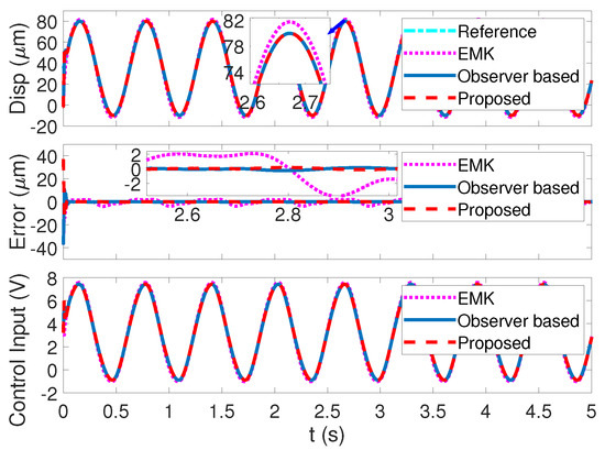
Figure 13.
Experimental results of the three control methods ().
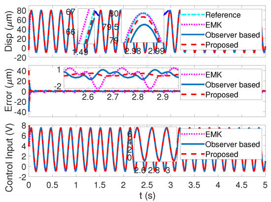
Figure 14.
Experimental results of the three control methods ().
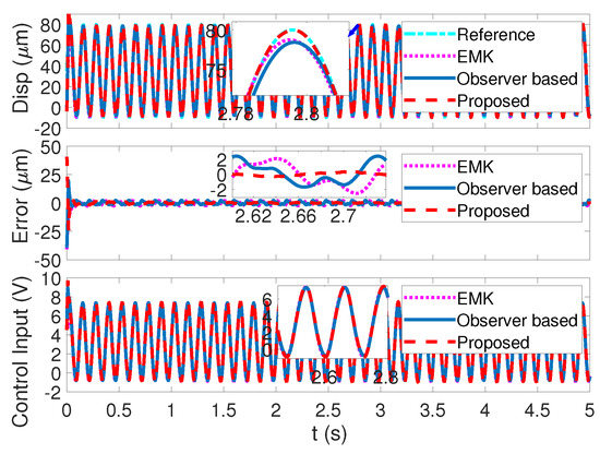
Figure 15.
Experimental results of the three control methods ().
Table 2.
The mean absolute errors (MAEs) of the three control methods.
Based on the above experimental result analysis, the proposed control strategy overwhelms the other two methods in tracking accuracy as a result of the drift disturbance compensated for by the observer and the unmodeled dynamics compensated for by the repetitive learning technology. Moreover, the advantage of the control method proposed in this paper widens as the tracking speed increases. Taking comparisons between the control method proposed in this paper and the observer-based control algorithm as an example, in , the mean absolute error (MAE) of the control methods in are 0.1418 m and m by the proposed method and the observer-based method, respectively, which reveals that the tracking error with the observer-based method is 1.13 times that of the proposed method. In , the absolute averages of the tracking errors in are 0.2885 m and m by the proposed method and the observer-based method, respectively, which reveals that the tracking error with the observer-based method is 1.81 times that of the proposed method. In , the absolute averages of tracking errors in are 0.4274 m and 1.1927 m by the proposed method and the observer-based method, respectively, which reveals that the tracking error with the observer-based method is 2.79 times that of the proposed method. Through the experimental error analysis above, the ratio of the tracking error with the observer-based method to that with the proposed method increases as the tracking angular velocity rises, which further demonstrates the high performance of the proposed method, especially in tracking relatively high speed signals.
The hysteresis loop compensation results of the reference sinusoid signal with , and are shown in Figure 16, Figure 17 and Figure 18. It is clear that the large hysteresis of the piezoelectric actuators in the open-loop status is effectively compensated for by the proposed strategy. Moreover, it can be seen from the figures that the linearity of the input/output with is the highest and the linearity with 50 rad/s is a bit lower compared with the two other results, which corresponds to the absolute average of the tracking errors distribution from to .
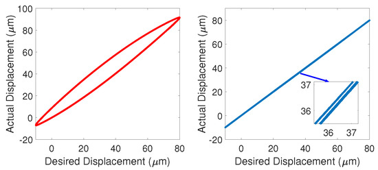
Figure 16.
Hysteresis loops in generated with open-loop status (left) and closed-loop status via the proposed strategy (right).
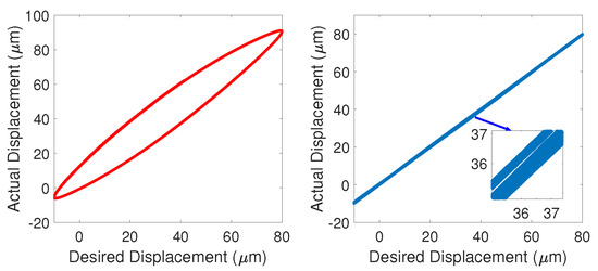
Figure 17.
Hysteresis loops in generated with open-loop status (left) and closed-loop status via the proposed strategy (right).
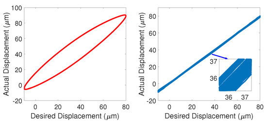
Figure 18.
Hysteresis loops in generated with open-loop status (left) and closed-loop status via the proposed strategy (right).
7. Conclusions
In this paper, a novel discrete compound compensation strategy, combining feedforward control with feedback control, is proposed to eliminate the system error mainly caused through the system hysteresis nonlinearity and the disturbances when tracking large travel range periodic signal. In the feedforward controller, a novel offline calibrate method is designed to eliminate the static hysteresis disturbance. A novel composite feedback control strategy, which is composed of a nonlinear observer and a repetitive learning control law, is designed to compensate for the dynamic hysteresis, the drift disturbance, and the system unmodeled uncertainty. The globally uniformly ultimately bounded (GUUB) stability of the control system is proved via the Lyapunov-based method. The high performance of the whole discrete compound compensation strategy is validated by simulations and experiments. Contrasts with two traditional control algorithms are performed and the outstanding performance of the control strategy proposed in this paper is verified by the results of tracking large range periodic signals with different angular velocities.
Author Contributions
Conceptualization, C.L. and Y.W.; methodology, C.L. and Y.F.; software, C.L. and Z.F.; validation, C.L., Y.F. and Y.W.; formal analysis, C.L.; investigation, C.L. and Z.F.; resources, C.L. and Z.F.; data curation, C.L. and Z.F.; writing—original draft preparation, C.L.; writing—review and editing, Y.F. and Y.W.; visualization, C.L. and Z.F.; supervision, Y.F.; project administration, Y.F. and Y.W.; funding acquisition, Y.W. All authors have read and agreed to the published version of the manuscript.
Funding
This research was funded by National Natural Science Foundation of China, grant number 62003172.
Data Availability Statement
All data are available in the manuscript.
Conflicts of Interest
The authors declare no conflict of interest.
References
- Binnig, G.; Quate, C.F.; Gerber, C. Atomic force microscope. Phys. Rev. Lett. 1986, 56, 930–933. [Google Scholar] [CrossRef] [PubMed]
- Xie, H.; Zhang, H.; Song, J.; Meng, X.; Wen, Y.; Sun, L. Highprecision automated micromanipulation and adhesive microbonding with cantilevered micropipette probes in the dynamic probing mode. IEEE/ASME Trans. Mechatron. 2018, 23, 1425–1435. [Google Scholar] [CrossRef]
- Brown, B.; Picco, L.; Miles, M.; Faul, C. Opportunities in high-speed atomic force microscopy. Small 2013, 9, 3201–3211. [Google Scholar] [CrossRef] [PubMed]
- Gu, G.; Zhu, L.; Su, C.; Ding, H.; Fatikow, S. Modeling and control of piezo-actuated nanopositioning stages: A survey. IEEE Trans. Autom. Sci. Eng. 2016, 13, 313–332. [Google Scholar] [CrossRef]
- Qin, Y.; Tian, Y.; Zhang, D.; Shirinzadeh, B.; Fatikow, S. A novel direct inverse modeling approach for hysteresis compensation of piezoelectric actuator in feedforward applications. IEEE/ASME Trans. Mechatron. 2013, 18, 981–989. [Google Scholar] [CrossRef]
- Chen, X.; Su, C.; Li, Z.; Yang, F. Design of implementable adaptive control for micro/nano positioning system driven by piezoelectric actuator. IEEE Trans. Ind. Electron. 2016, 63, 6471–6481. [Google Scholar] [CrossRef]
- Gu, G.; Zhu, L. Motion control of piezoceramic actuators with creep, hysteresis and vibration compensation. Sens. Actuators A Phys. 2013, 197, 709–717. [Google Scholar] [CrossRef]
- Padthe, A.; Drincic, B.; Oh, J.; Rizos, D.; Fassois, S.; Bernstein, D. Duhem modeling of friction-induced hysteresis. IEEE Control Syst. Mag. 2008, 28, 90–107. [Google Scholar]
- Zhou, J.; Wen, C.; Zhang, C. Adaptive backstepping control of a class of uncertain nonlinear systems with unknown backlash-like hysteresis. Automatica 2004, 49, 1751–1759. [Google Scholar] [CrossRef]
- Ismail, M.M.; Ikhouane, F.; Rodellar, J. The hysteresis Bouc-Wen model, a survey. Arch. Comput. Methods Eng. 2009, 16, 161–188. [Google Scholar] [CrossRef]
- Ding, B.; Li, Y.; Xiao, X.; Tang, Y. Optimized PID tracking control for piezoelectric actuators based on the Bouc-Wen model. In Proceedings of the IEEE International Conference on Robotics and Biomimetics, Qingdao, China, 3–7 December 2017; p. 16709742. [Google Scholar]
- Mayergoyz, I. Mathematical Models of Hysteresis and Their Applications; Elsevier: New York, NY, USA, 2003. [Google Scholar]
- Wu, Y.; Fang, Y. Hysteresis modeling with deep learning network based on Preisach model. Control. Theory Appl. 2018, 35, 723–731. (In Chinese) [Google Scholar]
- Wu, Y.; Fang, Y.; Liu, C.; Fan, Z.; Wang, C. Gated recurrent unit based frequency-dependent hysteresis modeling and end-to-end compensation. Mech. Syst. Signal Process. 2020, 136, 106501. [Google Scholar] [CrossRef]
- Yang, L.; Wang, Q.; Xiao, Y.; Li, Z. Hysteresis modeling of piezoelectric actuators based on a T-S fuzzy model. Electronics 2022, 11, 2786. [Google Scholar] [CrossRef]
- Liu, J.; Shan, Y.; Qi, N. Creep modeling and identification for piezoelectric actuators based on fractional-order system. Mechatronics 2013, 23, 840–847. [Google Scholar] [CrossRef]
- Mokaberi, B.; Requicha, A.A.G. Drift compensation for automatic nanomanipulation with scanning probe microscopes. IEEE Trans. Autom. Sci. Eng. 2006, 3, 199–207. [Google Scholar] [CrossRef]
- Li, G.; Wang, Y.; Liu, L. Drift compensation in AFM-based nanomanipulation by strategic local scan. IEEE Trans. Autom. Sci. Eng. 2012, 9, 755–762. [Google Scholar] [CrossRef]
- Wu, Y.; Zou, Q. Robust inversion-based 2-DOF control design for output tracking: Piezoelectric-actuator example. IEEE Trans. Control Syst. Technol. 2009, 17, 1069–1082. [Google Scholar]
- Ren, J.; Zou, Q. A control-based approach to accurate nanoindentation quantification in broadband nanomechanical measurement using scanning probe microscope. IEEE Trans. Nanotechnol. 2014, 13, 46–54. [Google Scholar] [CrossRef]
- Wang, J.; Zou, Q. Rapid probe engagement and withdrawal with force minimization in atomic force microscopy: A learning-based online-searching approach. IEEE/ASME Trans. Mechatron. 2020, 25, 581–593. [Google Scholar] [CrossRef]
- Nguyen, M.; Chen, X.; Yang, F. Discrete-time quasi-sliding-mode control with prescribed performance function and its application to piezo-actuated positioning systems. IEEE Trans. Ind. Electron. 2018, 65, 942–950. [Google Scholar] [CrossRef]
- Nguyen, M.; Chen, X. MPC inspired dynamical output feedback and adaptive feedforward control applied to piezo-actuated positioning systems. IEEE Trans. Ind. Electron. 2020, 67, 3921–3931. [Google Scholar] [CrossRef]
- Yong, Y.K.; Moheinami, S.O.R.; Kenton, B.J.; Leang, K.K. Invited review article: High-speed flexure-guided nanopositioning: Mechanical design and control issues. Rev. Sci. Instrum. 2012, 83, 121101. [Google Scholar] [CrossRef] [PubMed]
- Baziyad, A.; Ahmad, I.; Salamah, Y.; Alkuhayli, A. Robust tracking control of piezo-actuated nanopositioning stage using improved inverse LSSVM hysteresis model and RST controller. Actuators 2022, 11, 324. [Google Scholar] [CrossRef]
- Song, G.; Zhao, J.; Zhou, X.; Abreu-Garcia, J.A.D. Tracking control of a piezoceramic actuator with hysteresis compensation using inverse Preisach model. IEEE/ASME Trans. Mechatron. 2005, 10, 198–209. [Google Scholar] [CrossRef]
- Shan, Y.; Leang, K.K. Accounting for hysteresis in repetitive control design: Nanopositioning example. Automatica 2012, 48, 1751–1758. [Google Scholar] [CrossRef]
- Fang, Y.; Feemster, M.; Dawson, D.; Jalili, N. Nonlinear control techniques for an atomic force microscope system. Control. Theory Appl. 2005, 3, 85–92. [Google Scholar] [CrossRef]
- Gu, G.; Zhu, L.; Su, C. High-precision control of piezoelectric nanopositioning stages using hysteresis compensator and disturbance observer. Smart Mater. Struct. 2014, 23, 105007. [Google Scholar] [CrossRef]
- Levant, A. Higher-order sliding modes, differentiation and outputfeedback control. Int. J. Control 2003, 76, 924–941. [Google Scholar] [CrossRef]
- Ding, B.; Li, Y. Hysteresis compensation and sliding mode control with perturbation estimation for piezoelectric actuators. Micromachines 2018, 9, 241. [Google Scholar] [CrossRef]
- Xu, Q. Continuous integral terminal third-order sliding mode motion control for piezoelectric nanopositioning system. IEEE/ASME Trans. Mechatron. 2017, 22, 1828–1838. [Google Scholar] [CrossRef]
- Dang, X.; Tan, Y. RBF neural networks hysteresis modelling for piezoceramic actuator using hybrid model. Mech. Syst. Signal Process. 2007, 21, 430–440. [Google Scholar] [CrossRef]
- Chen, W.; Ballance, D.; Gawthrop, P.; O’Reilly, J. A nonlinear disturbance observer for robotic manipulators. IEEE Trans. Ind. Electron. 2000, 47, 932–938. [Google Scholar] [CrossRef]
- Feemster, M.; Fang, Y.; Dawson, D. Disturbance rejection for a magnetic levitation system. IEEE/ASME Trans. Mechatron. 2006, 11, 709–717. [Google Scholar] [CrossRef]


Publisher’s Note: MDPI stays neutral with regard to jurisdictional claims in published maps and institutional affiliations. |
© 2022 by the authors. Licensee MDPI, Basel, Switzerland. This article is an open access article distributed under the terms and conditions of the Creative Commons Attribution (CC BY) license (https://creativecommons.org/licenses/by/4.0/).