Abstract
Rail surface defects will not only bring wheel rail noise during train operation, but also cause corresponding accidents. Most of the existing detection methods are manual detection, which is time-consuming, laborious, inefficient, and subjective. With the development of technology, automatic detection replaces manual detection, which reduces manual labor, improves efficiency, and objectively evaluates the surface state of rails, which is in line with the purpose of modern intelligent production. The automatic detection of a single sensor is usually not enough to complete the recognition, but multiple sensors need to be additionally installed and refitted on the service vehicle, which creates difficulty for on-site test conditions. Therefore, in order to overcome these shortages and to adapt to the actual vibration characteristics of service vehicles, a rail surface defect recognition method based on optimized VMD gray image coding and DCNN is proposed in this paper. Firstly, the optimization method of VMD mode number based on the maximum envelope kurtosis is proposed. The VMD after parameter optimization is used to decompose the four-channel axle box vibration signal, and the component with the largest correlation coefficient between each order eigenmode component and the original signal is extracted. Secondly, the filtered IMF components are arranged in sequence and encoded into grayscale images. Finally, the DCNN structure is designed, and the training set is input into the network for training, and the test set verifies the effectiveness of the network and realizes the recognition of rail surface defects. The test accuracy of railway data set measured on the serviced vehicle is 99.75%, and the results show that this method can accurately identify the category of rail surface defects. After adding Gaussian noise to the original signal, the test accuracy reaches 99.20%, which proves that the method has good generalization ability and anti-noise performance. Additionally, this method can ensure the safe operation of vehicles without adding new equipment, which reduces operation costs and improves the intelligent operation and maintenance of rails.
1. Introduction
With the improvement of railway speed, the safety of high-speed railway has become a hot research topic, and the defects recognition of rail is the most essential aspect. Surface defects associated with rolling contact fatigue (RCF) damage, such as squats [1], studs [2], and head check valves [3]. The existence of rail surface defects also increases the vertical dynamic load of wheel set on the rail and aggravates the deterioration of track and some vehicle components. If the rail surface defect is not treated, it may lead to complete rail failure [4,5].
Several manual and automatic methods have been applied in rail surface inspection during engineering project. Traditional railway surface inspection adopts manual inspection [6], e.g., via hammering and shocking [7], which is inefficient and highly relies on the experience and ability of personnel, and it is difficult to ensure the accuracy of detection results. Since with the development of technology, the automatic inspection based on vibration and acoustic have been introduced to deal with the rail fault [8]. Moreover, with the concept proposal of intelligence operation and maintenance algorithm, ultrasonic detection [9], ultrasonic guided wave detection [10], eddy current detection [11], and magnetic flux leakage detection [12] have been progressed into the rail inspection.
As mentioned above, rail surface defects contain different types, such as rolling contact fatigue of turnout, rail squats, void zones, and unsupported sleepers/bears. Therefore, several sources of research have attempted to deal with these problems, and some of them have integrated with ESAH-M, ESAH-F systems. Most of them analyze the parameters of rolling contact fatigue [13] and the dynamic phenomena of turnout [14], dynamic response [15], impact and residual settlements accumulation [16], wheel load reduction [17], and stress state [18] under unsupported sleepers, rail squat characteristics [19] via dynamitic and finite element modelings. According to these sources, the causes, variation, and effects of the rail surfaces defects can be analyzed and monitored. The targets being inspected here are the rail surfaces for high-speed trains. The tracks used for high-speed trains are ballastless tracks, and several analyses mentioned above focus on ballasted tracks. Thus, the calculated parameters may not be suitable for this simulation, but the methods can still be referred. In reference [19], they have done the rail squat characteristics under train axle box acceleration frequency (ABA) by using wavelet scattering, which is similar to the inspection requirements. However, the types of the tracks and operating conditions in [19] do not match with those for high-speed trains.
After the principle of intelligent maintenance introduced, operators will more often use the track inspection vehicle to carry out daily automatic detection of rail defects [20].
However, these diagnostic devices on track inspection vehicles cannot be installed on the service vehicle, once a serious rail defect occurs during running conditions, an accident cannot be avoided. The present automatic inspection also needs to install or apply auxiliary sensors or instruments to achieve the target of rail surface defects inspection [21]. Therefore, it is necessary to come out a systematic rail surface defects inspection method without installing any extra devices and be suitable for service vehicles.
The rail surface inspection base on vision inspections has recently been applied in railway condition monitoring research. Model-based approaches and data-driven approaches are two categories of techniques heavily discussed in the literature of inspecting rail defects. In the model-based approaches, explicit models including thresholding and texture models were applied to handle the image segmentation and analysis [8,22]. In the category of data-driven approaches, image processing methods are widely used in rail surface defects [23,24], such as image level detection [1], image position detection [2], and pixel-level segmentation detection [3], which has been proposed because of its fast and intuitive. With the continuous development of artificial intelligence technology, BP neural network [25], PNN [26], support vector machine (SVM) [27], deep convolutional neural network (DCNN) [28], and machine vision [29,30] have been widely used in the field of defects recognition. Among them, the use of deep learning realizes the automatic recognition of rail surface defects [29,30]. As one of the main methods, convolutional neural network (CNN) [31,32] is widely used in the field of rail image recognition and has achieved excellent results.
In real engineering projects and daily operations, most operating defects of railways would be collected and recorded via mounted and pre-installed sensors and all the data measured would be transferred and imported into a vehicle diagnostic system [33]. Due to the convenience and reliability of vibration inspection, it has been widely used in vehicle fault recognition [4], which also provides the possibility and reference for analyzing track defects by using the obtained vibration data. Usually, the collected vibration signal contains background noise, and the vibration signal has non-stationary and nonlinear characteristics. How to extract effective features from the vibration signal is the key to rail surface defects recognition. Several signal processing methods, such as empirical mode decomposition (EMD) [5], time-frequency analysis [33], singular value decomposition (SVD) [34], etc., decompose different signals into different components through signal characteristics, and analyze the signals in each component. However, these algorithms also have some problems. EMD is limited by endpoint effect and mode aliasing [35]. Dragomiretskiy et al. [36] proposed a non-stationary signal processing method: variational mode decomposition (VMD), which overcomes the above problems in EMD method [37,38].
So far, several strategies have been processed on rail inspection via sensors. The mechanical wear contact between wheel and rail on a turnout has been studied [39]. Railroad turnout diagnostics has been made based on mounted rail tracks acceleration sensors [40]. With the development of simulation, the conditions of crossing geometry of rail are also analyzed based on track responses [41]. Moreover, due to the rise of neural networks, deep learning networks are applied on the measurement and analysis of segmentation surface of railway tracks [42]. However, these measurements are collected at the rail trackside, or inspecting vehicles. There is bound to be a difference between the measured value under above ways and the actual operating state of the service vehicle.
Therefore, how to maximize the use of vehicle pre-installed multi-sensor monitoring or measuring data and use processing and analysis methods adapted to actual operating data to obtain track surface status or defect characteristics is a problem worthy of further in-depth study. Aiming at the problem that the information reflected by a single sensor is not comprehensive, multi-sensor information fusion is used to provide more information for target detection [43,44,45,46].
To sum up, theoretically, this paper proposes a method to construct a DCNN rail surface defect recognition model by using multi-channel vibration signals to gray-scale coding after optimized VMD processing. The method realizes denoising and interference elimination of multi-channel vibration data fusion and rail surface defect detection. In engineering, this method can apply rail defects recognition without pre-installing and modifying any auxiliary devices on service vehicles.
The chapters of this paper are arranged as follows: after the introduction, Section 2 studies the proposed optimized VMD and DCNN methods. In Section 3, the four classification and two classification tests are verified and the results are analyzed through the field measured data. Finally, the anti-noise performance and stability of the proposed method are verified through the anti-noise performance test. Section 4 is the conclusion of the full text.
2. The Proposed Optimized VMD and DCNN Methods
From the foregoing, the goal of this paper is to design a method suitable for the following situations, using the multi-channel vibration sensor pre-installed on the service vehicle to collect the signal data under the actual operating state, carry out effective analysis, obtain the characteristics of the track surface and then establish a rail surface defect identification model. So, considering that it is difficult to extract the features of rail surface defects and the information reflected by a single sensor is not comprehensive, a multi-sensor fusion rail surface defects recognition method based on optimized VMD grayscale image coding and DCNN is proposed to realize rail surface defects recognition.
2.1. General Procedures of the Proposed Method
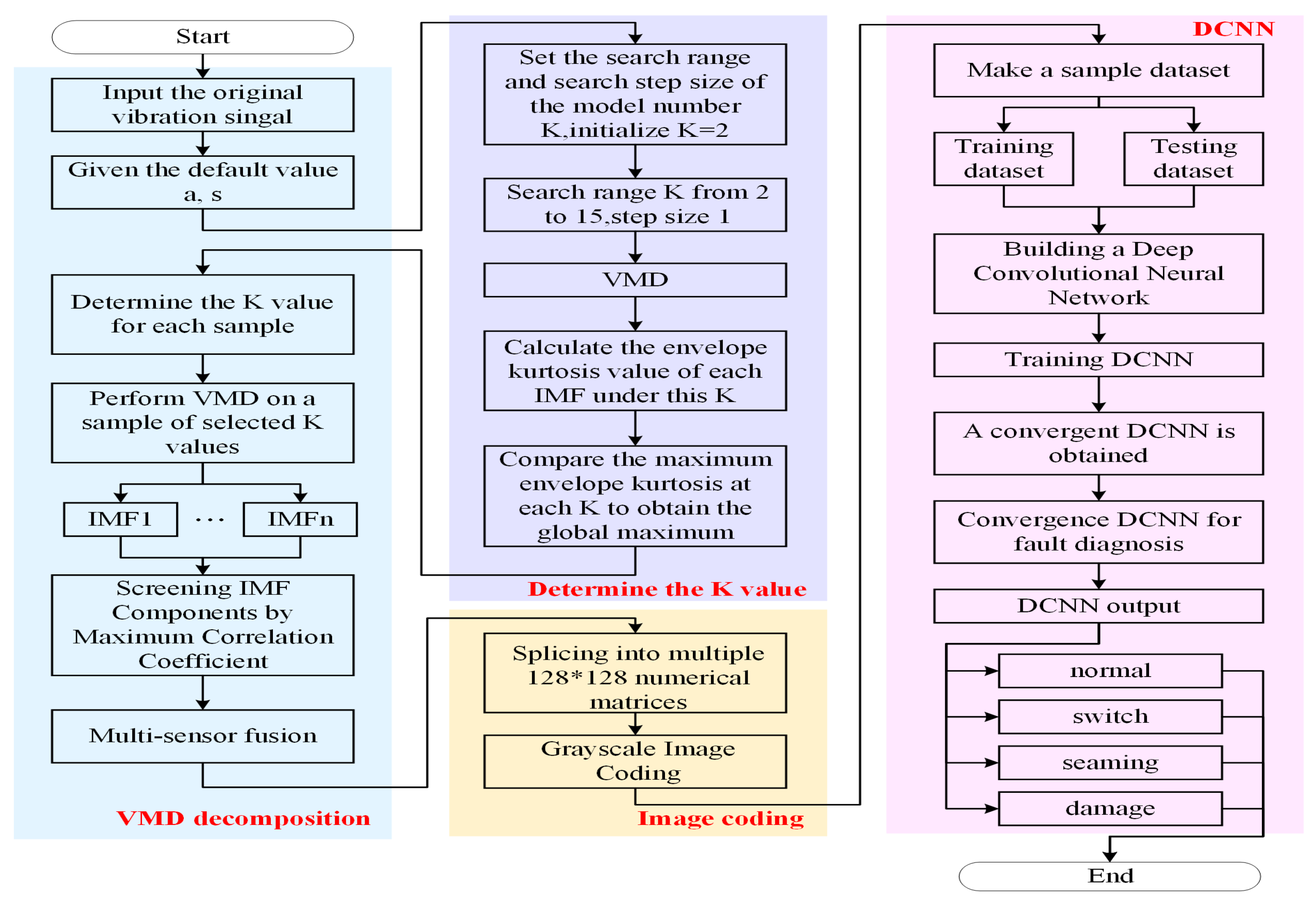
Based on the construction of “2.4” section grayscale image coding based on VMD-multi-sensor fusion and “2.5” section construction of convolutional neural network, this paper proposes a multi-sensor fusion rail surface defects recognition method based on VMD grayscale image coding and DCNN. Figure 1 is the overall algorithm flow chart.
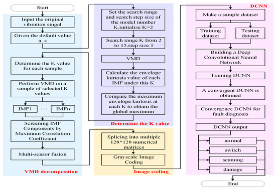
Figure 1.
Overall algorithm flow chart.
The specific data processing steps are as follows:
- (1)
- Divide the original vibration signal data collected by the axle box four channel sensor at equal intervals, and make the sample data set;
- (2)
- Select K ϵ [2, 15] as the search domain of the VMD mode number and calculate the maximum value of envelope kurtosis under each mode number for each sample so as to determine the optimal mode number of VMD under this sample;
- (3)
- VMD decomposition is carried out for each sample, and the IMF component after decomposition is screened by using the correlation coefficient;
- (4)
- The IMF components with the largest correlation coefficient between the eigenmode components of each order and the original signal are extracted and normalized, and the IMF components screened by multiple sensors are arranged in turn to form a numerical matrix;
- (5)
- Convert the numerical matrix in step 4 into a grayscale image and generate several grayscale images from the time series data of the four rail surface defects according to the above steps, as the data set for DCNN training and testing;
- (6)
- Randomly divide the training set and the test set, use the training set to train the convolutional neural network, and at the same time optimize and adjust the network structure and network parameters according to the training results during the training process;
- (7)
- The test set is used to verify the effectiveness of convolutional neural network and predict the image classification results so as to obtain the defects recognition of rail vibration signal, output the recognition results and analyze the conclusions.
2.2. Determination of the Mode Number of VMD
Several vibration signal processing methods have been introduced and mentioned in literature review, but only VMD can be adapted and is suitable for rail inspection. The core of the denoising progress is to extract the feature or useful information and devote the noise into different parts or layers [47,48,49]. Therefore, VMD is based on Wiener filtering theory, which can be used here. VMD is a completely non recursive variational mode decomposition model. In this algorithm, the intrinsic mode function (IMF) is defined as a bandwidth limited AM-FM function. VMD algorithm decomposes the original signal into a specified number of IMF components by constructing and solving the constrained variational problem. Before VMD decomposition of the signal, the parameters of VMD need to be determined, that is, the mode number and penalty factor need to be determined in advance. After determining the influence parameters, the signal is decomposed by VMD to obtain a series of intrinsic mode functions (IMFs) [47,48].
This paper presents a novel method to calculate the kurtosis value from the Hilbert transform (HT) to effectively optimize and determine the mode number of VMD. The default values of the penalty factor and bandwidth, α = 2000, s = 0 [43], the initial mode number is set as k = 2. In order to determine the search range and step size of the mode number K, the paper draws on the discussion range of the mode number K derived from reference [44]. If K is too large, the efficiency is low, and the calculation load is heavy. If K is too small, it is easy to introduce noise. So, choose K ϵ [2, 15] is used as its search domain, the step size is set to 1.
VMD analysis is performed on the collected vibration signal, calculating the envelope kurtosis value of each modal signal under the set mode number and obtaining the maximum value of the envelope kurtosis under the mode number through comparison, then to continue the above analysis until , and finally obtain the maximum value of the envelope kurtosis under each mode number.
Assuming that the mode number of the VMD is , the envelope of each mode can be calculated, i.e.,
where represents the mode of , is the absolute value (the result of HT of the mode of ), represents the mode generated by VMD when the mode number is ().
Further, the envelope kurtosis of the mode of is calculated as follow:
where denotes the mean of , and denotes the standard deviation of , the numerator of Formula is the fourth-order central moment of .
Then, a local maximum can be obtained,
Since the search interval of is set to and the search step is set to 1, 14 local maximum can be obtained in the entire search interval. Then, the global maximum can be obtained:
Thus, the mode number selected based on the maximum , and it is expressed as , can be obtained from the formula :
2.3. The Selection of the Sensitive IMF of VMD
The IMF components obtained by VMD method include the local characteristics of the original signal at different time scales [45,46]. The first few IMF components reflect the main characteristics of the original signal. In order to ensure that the constructed grayscale image can effectively retain the state characteristics of the original signal and avoid the interference of noise and other components, the correlation coefficient method is used to screen the decomposed IMF components, and the IMF component with the largest correlation coefficient is used as the data to generate the grayscale image. The calculation formula of correlation coefficient is as follows [36]:
where is the signal length; is the correlation coefficient between the IMF component and the original signal .
2.4. GRAYSCALE Image Coding Based on VMD
Rail vehicles contain strong background noise in actual work, which makes it difficult to obtain comprehensive state characteristics by analyzing the signal measured by a single sensor, which affects the accuracy of state recognition, and the selection of better sensor location depends on the practical test experience of experimenters. Therefore, at the feature level, this paper arranges the filtered IMF components in turn and converts them into grayscale images. The grayscale image coding is shown in Figure 2.
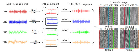
Figure 2.
Grayscale image encoding process.
The main steps of grayscale image coding based on VMD are as follows:
- (1)
- The original vibration signals , , and measured by the four channel sensors are divided into equidistant segments with a distance of ;
- (2)
- VMD the segmented signal;
- (3)
- Screened the IMF component with the largest correlation coefficient;
- (4)
- Assuming the size of the grayscale image to be constructed as (generally , , , etc.), divide the width into 4 equal parts, construct 4 regions of , and fill the IMF components filtered by each sensor signal in turn according to the size of the region;
- (5)
- Encode the numeric matrix into a grayscale image.
In order to better compare the grayscale images, the filtered IMF components are normalized. The normalization formula is as follows:
where , represents the values before and after normalization, respectively; , are the maximum value and the minimum value of the original grayscale image, respectively.
2.5. Convolutional Neural Network Construction
In order to effectively identify the gray images of various rail surface defects, it is necessary to design a reasonable DCNN. DCNN is tested by controlling variables to determine the structure and parameters of the final network. The experimental grouping is shown in Table 1 below.

Table 1.
Experiment grouping situation.
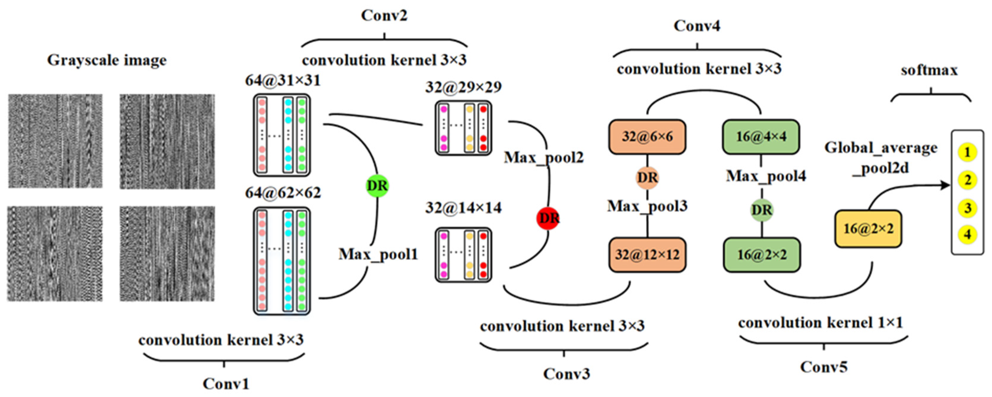
Through the data set, each group of networks designed in Table 1 are trained, tested, and compared one by one, and the network structure is finally determined. The convolutional neural network has a total of 15 layers, including 5 convolutional layers, 4 pooling layers, 4 random deactivation layers, 1 global average pooling layer, 1 softmax layer for classification, that is, the output layer, use 3 × 3 convolution kernel, the last convolutional layer adopts a 1 × 1 convolution kernel and uses ReLU as the activation function to adjust the classification output results after the global average pooling layer to 4 categories. The structure diagram of deep convolutional neural network is shown in Figure 3, and the parameters of each layer are shown in Table 2.
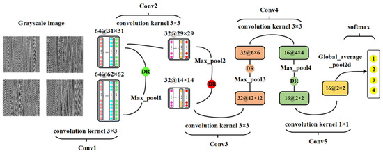
Figure 3.
Deep convolutional neural network structure diagram.
Table 2.
The structure and parameters of the DCNN networks.
3. Validation and Discussion
3.1. Measured Data Set Result Analysis (Four Categories)
3.1.1. Experimental Data
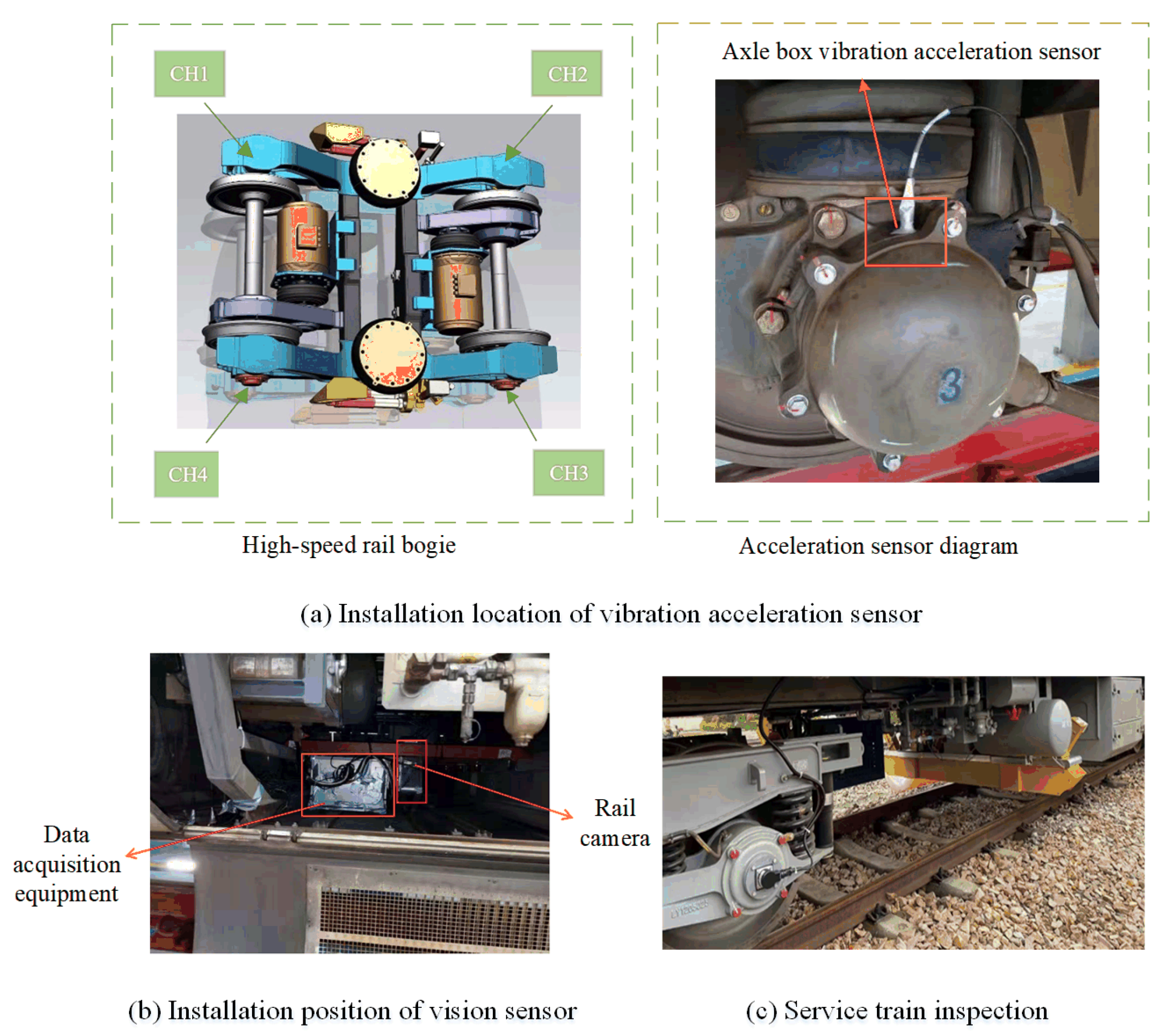
The data in this paper comes from the measured data of axle box vibration acceleration of high-speed trains on Shanghai Nanjing intercity uplink and downlink lines. The test time is from 23 to 24 December 2020, the sampling frequency is 12,800 hz, and the data was saved every 1 h. The data range is 19:00:00–23:59:59 on 23 December 2020 and 19:00:00–23:59:59 on 24 December 2020. The test equipment adopts four vibration acceleration sensors and one visual sensor. All the parameters of sensors during measurements have been indicated in Table 3. According to those characteristics of the sensors, the installation position of the test equipment and sensors is shown in Figure 4. The vibration acceleration sensor simulates the pre-installed vibration sensor on the axle box of the service vehicle, and the vision sensor can simultaneously collect the rail image, which is convenient to provide a label reference for the vibration data during the production of the data set. The final rail defect identification model still only uses the vibration signal data of pre-installed and in-service vehicles.
Table 3.
The parameters of the sensors using in test measurements.
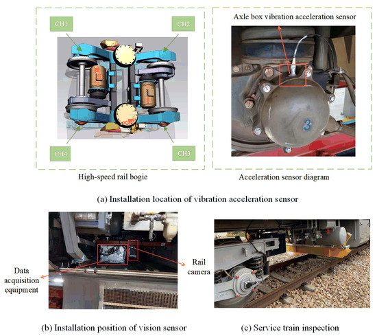
Figure 4.
Installation position of test equipment and sensors.
The uncertainty would be a problem for vibration and vision images measurement. All of the budgets of uncertainties [49] are shown in Table 4. It can be seen that the repeatability (Random) uncertainty is the biggest influence factor of measurements.
Table 4.
The uncertainties budgets in the test.
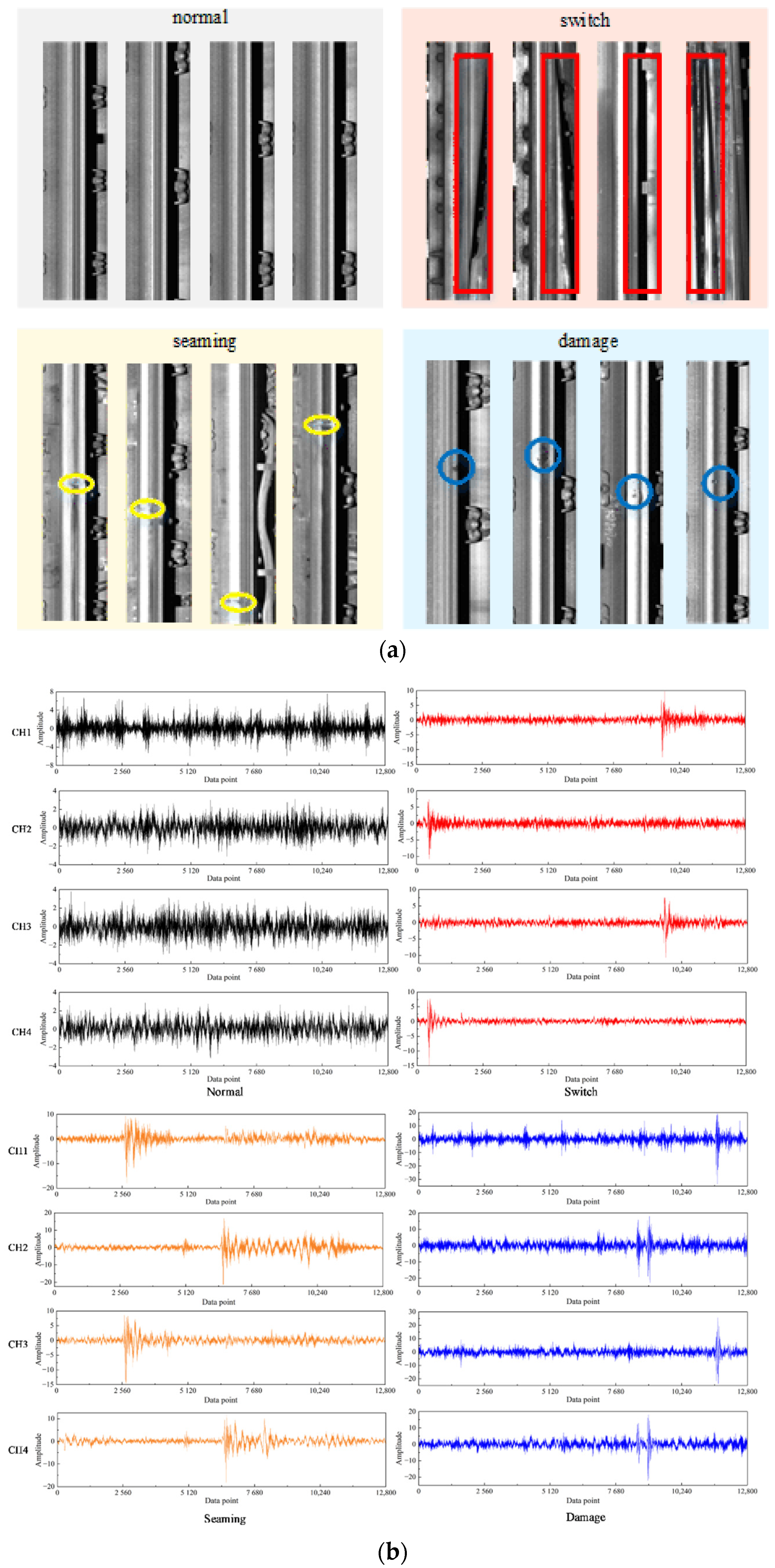
The images of special rail sections, such as switch, seaming, and damage are extracted by image recognition software, and the acquisition time corresponding to the image is obtained. According to the collected passing time of special section, extract the axle box vibration acceleration data corresponding to the image, and obtain four defect samples of rail surface, i.e., switch, seaming, damage, and normal. The four defect images of the rail surface are shown in Figure 5a, and the vibration signal waveforms of the four states are shown in Figure 5b.

Figure 5.
Schematic diagrams and waveforms of four sections under different four channels. (a) Schematic diagram of four sections. (b) Vibration signal waveform diagram.
For vibration signals, in order to find out the characteristics of rail surface defects, several features have been introduced and processed in rail surface inspections. Moreover, as a feature, it is necessary to have good sensitivity and stability during the evaluation. Therefore, the calculation formula and comparison of features sensitivity and stability are made and shown in Table 5. The envelope kurtosis has the best sensitivity and stability, compared with other features. Moreover, the identification accuracy of turnout, joint, or damage among different features are also processed in this Table. It can be seen that envelope kurtosis has the best identification accuracy performance compared with other existing features in turnout, joint, or damage conditions. Therefore, the envelope kurtosis here would be an appropriate feature for inspection of rail surface defects.
Table 5.
The comparison of features sensitivity, stability, calculation formula, and damage identification accuracy in rail surface inspection.
3.1.2. Analysis of the Mode Number of VMD
In the search domain, the relationship between the four channels mode number K and the maximum value of the envelope kurtosis is plotted in Figure 6. For the four defect samples of the rail surface, the maximum value of the envelope kurtosis can be obtained when each sample of the four channels takes the optimal mode number K’. The relationship is shown in Table 6.
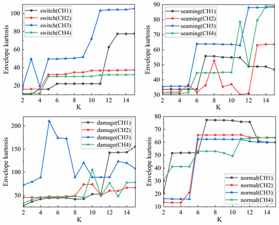
Figure 6.
K and local maximum envelope kurtosis.
Table 6.
Relationship between 4-channel K’ and global maximum envelope kurtosis.
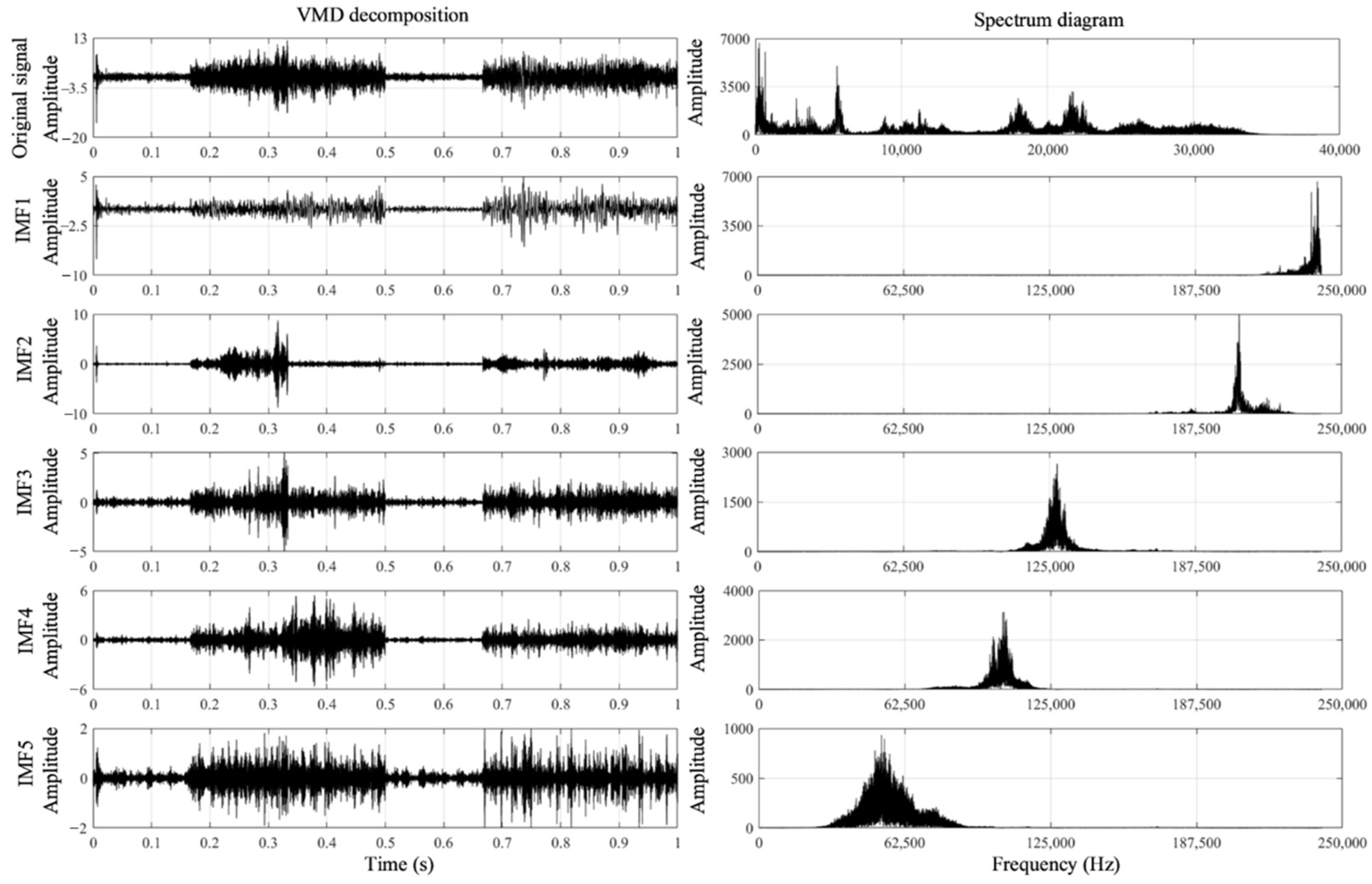
It can be seen from Table 3 that the specific samples correspond to the optimal mode number one to one, and give an example of VMD decomposition of a specific sample. For example, for switch CH4 sample 4, when K’ = 5, the envelope kurtosis is the largest. For sample 4, VMD with 5 modes is used to analyze the original signal. After VMD decomposition, five eigenmode functions are generated. The time domain representation of each IMF component in a channel is shown in Figure 7. In addition, due to the muti-sensors fusion, the reliability of different channels should also be discussed. In this sub-section, the performance and reliability of those four channels are presented by calculating the signal to noise ratio (SNR) and root mean square error (RMSE). All the calculated results have been indicated in Table 7. It can be seen that the CH1 have the smallest SNR in collected signals under the damage defect compared with other channels. Additionally, the CH4 is the relatively stable channel compared with other channels. Among those three defects, the SNRs under damage conditions are still the smallest compared with those in the switch and the joint. Similar to the results calculated by RMSE, the RMSE in the damage condition is the largest compared with other defect conditions.

Figure 7.
The vibration signal example after VMD decomposition in a channel.
Table 7.
The performance of different measurement channels under different defects.
For rail surface inspection, only SNR and RMSE may not show the practical performance during inspections. Therefore, the maximum information coefficient (MIC) also calculated and analyzed under different rail state. A total of 15 types of time domain characteristic parameters for four channels and four states are applied, respectively, and the correlations between CH1, CH2, CH3, and CH4 are calculated using the MIC. It can be seen from Table 8 that the minimum MIC value is 0.75, which is the MIC value between the switch states CH1 and CH4. According to the results, 0.75 is highly correlated. The four states of the four channels are highly correlated.
Table 8.
The maximum information coefficient (MIC) of different channels under different rail states.
3.1.3. Image Encoding Result
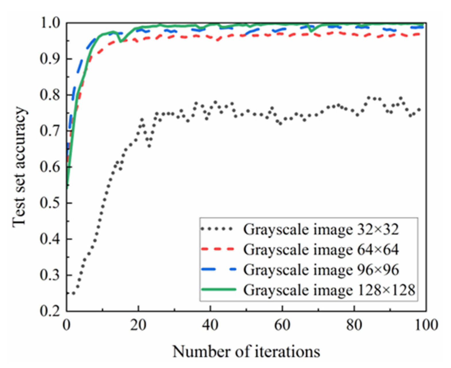
In the equidistant segmentation of the original vibration data, four cases with lengths of 32, 64, 96, and 128 are adopted. According to the grayscale image construction method, the grayscale images with pixels of 32 × 32, 64 × 64, 96 × 96 and 128 × 128 can be constructed from the signals with lengths of 32, 64, 96, and 128, respectively. The experiment is carried out with the measured axle box vibration data of the serviced vehicle. The vibration signals under four lengths are generated into grayscale images and input into the network for training. Figure 8 is the accuracy change curve of test sets with different pixel sizes. Among them, the grayscale image of 32 × 32 cannot distinguish the four types of rail surface defects because there are too few pixels and the image features are not obvious. The test accuracy of the grayscale image with 128 × 128 pixels is slightly higher than that of 96 × 96 and 64 × 64 pixels, and the convergence speed and stability of the test accuracy curve are better than that of the grayscale image with 96 × 96 and 64 × 64 pixels, which can better distinguish four types of defects. Considering comprehensively, the grayscale image with 128 × 128 pixels is finally used as the grayscale image pixel for DCNN training and testing.
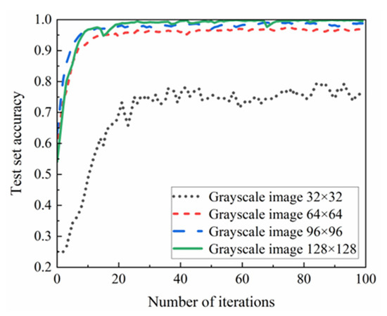
Figure 8.
Contrast of different pixel precision.
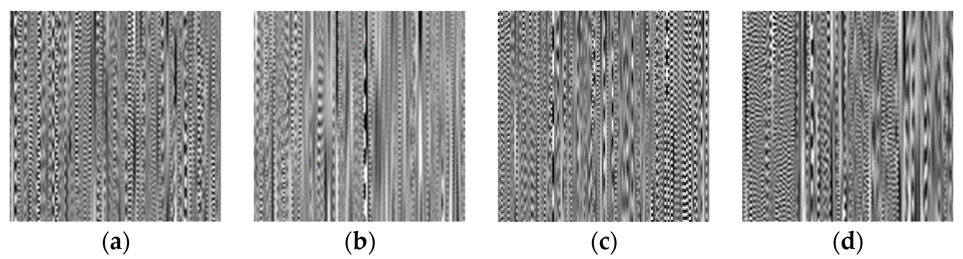
As can be seen from Figure 8, the grayscale image test accuracy curve with 128 × 128 pixels have faster convergence speed, better stability and higher test accuracy than the test accuracy curve with 32 × 32 pixels, 64 × 64 pixels and 96 × 96 pixels. Figure 9 shows the grayscale image with 128 × 128 pixels. It can be seen from Figure 9 that the grayscale images of four different defects constructed by the above method have significantly different feature.
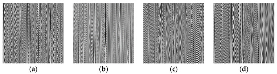
Figure 9.
Example of grayscale image. (a) Switch; (b) Seam; (c) Damage; (d) Normal.
3.1.4. Experimental Result and Analysis
According to the axle box vibration data of the serviced vehicle, a total of 3200 grayscale images are generated. The images are randomly assigned, and the assigned numbers of training set and test set in each defect are 640 and 160, respectively.
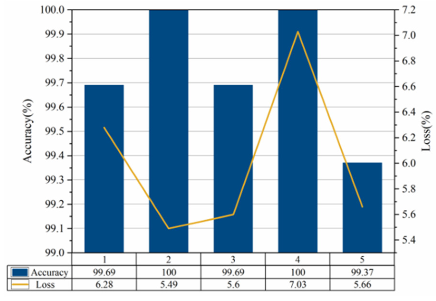
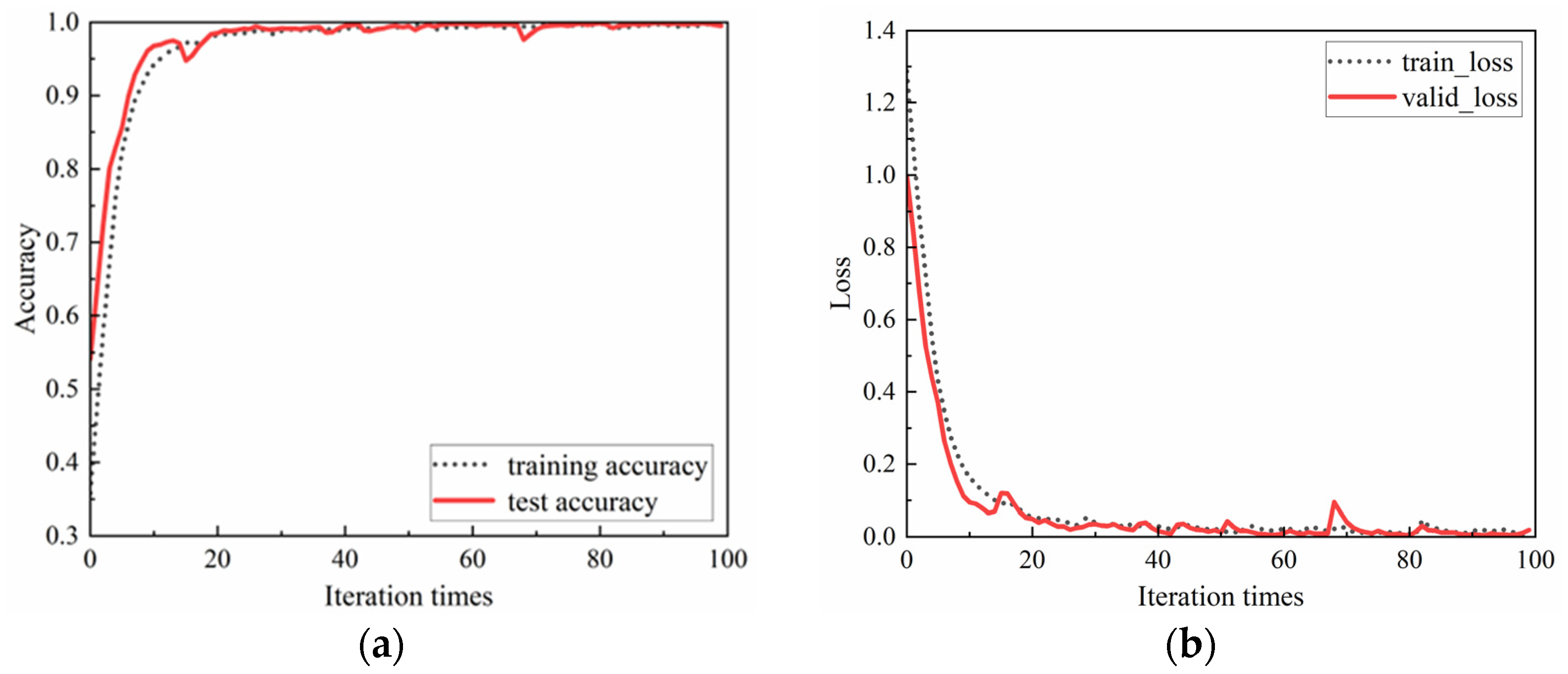
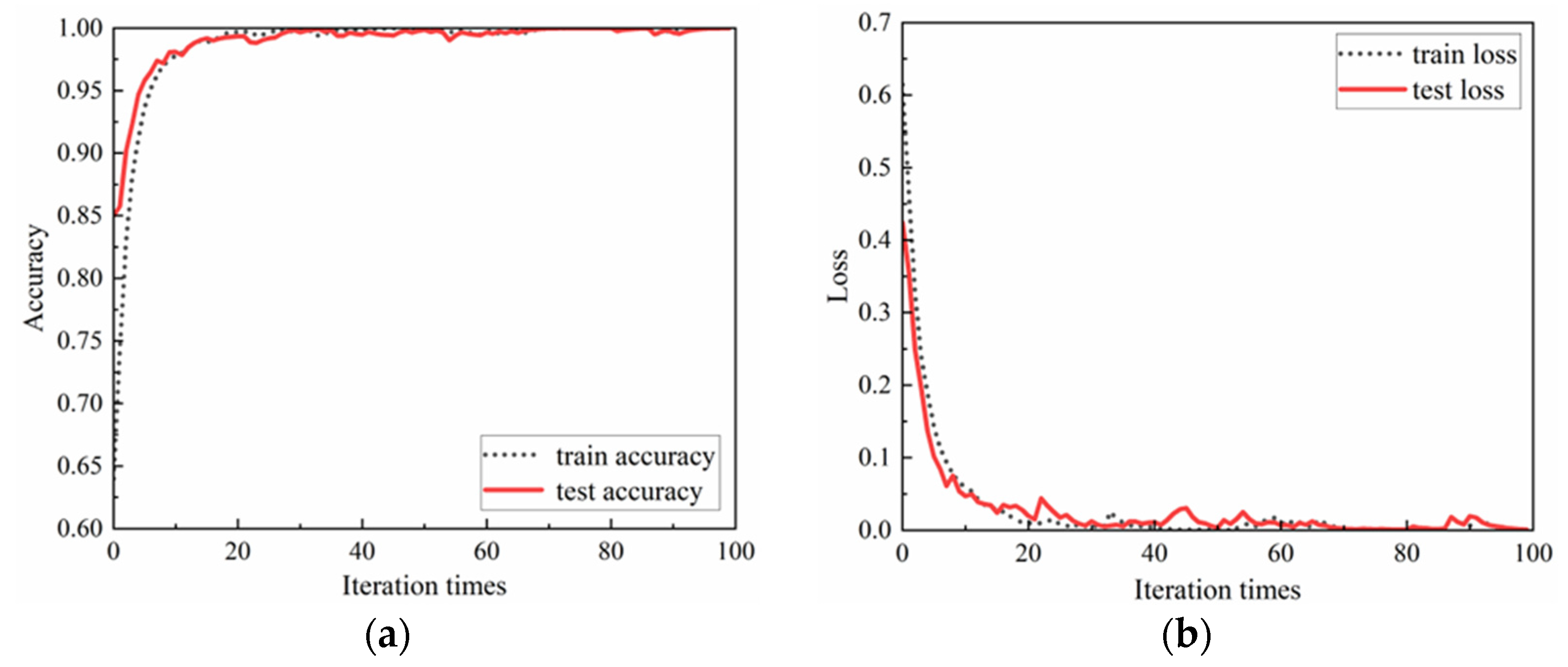
Run the network five times, and Figure 10 shows the identification accuracy and loss rate of the test set obtained from the five tests. Among them, the accuracy changes and loss change curves of the training set and test set in the fourth test are shown in Figure 11. In training, one iteration refers to the process that all data complete a forward calculation and back propagation in the network. The accuracy rate reflects the proportion of images correctly recognized by the model, and the loss rate is used to evaluate the inconsistency between the predicted value and the real value of the model. The greater the accuracy, the smaller the loss rate, the better the recognition ability and robustness of the model.
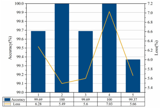
Figure 10.
Accuracy and loss rates for multiple tests.
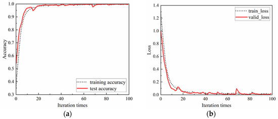
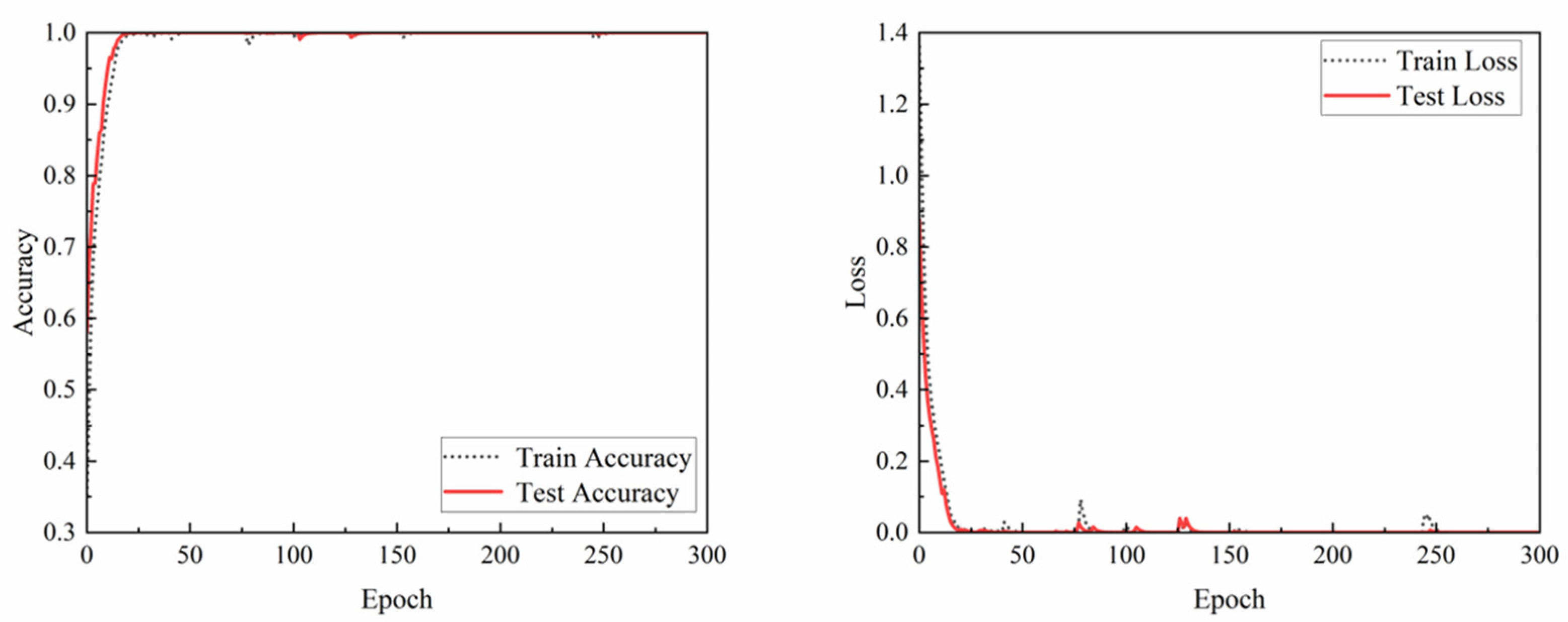
Figure 11.
Accuracy changes and loss changes of training set and test set. (a) Accuracy changes. (b) Loss changes.
By analyzing the data in Figure 10, the method proposed in this paper obtains good results. The average recognition accuracy of the test set of five tests is 99.75%. It can be seen that using the multi-sensor fusion rail surface defects recognition method based on VMD grayscale image coding and DCNN to analyze the rail vibration signal can effectively realize the rail surface defects recognition with a high stability.
It can be seen from Figure 11 that the accuracy curve rises rapidly and tends to be stable regardless of training or testing, and the loss curve decreases rapidly and tends to be stable. After 100 iterations, the final test accuracy and loss values are 100% and 7.03%, respectively.
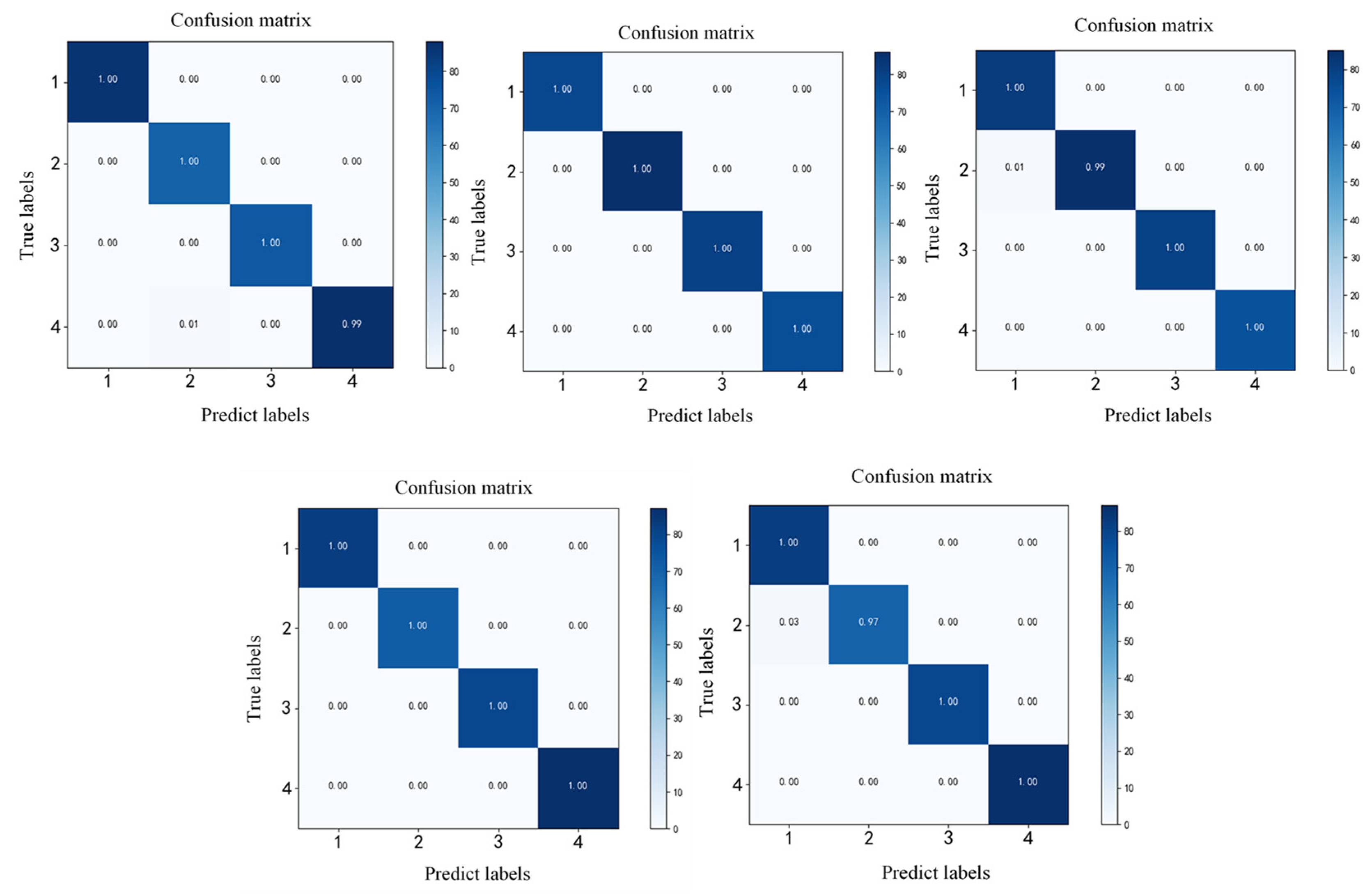
In order to represent the specific classification of rail surface defects of different categories, the confusion matrix of classification results is given. Figure 12 shows the confusion matrix of five test results. The horizontal axis represents the prediction category, the vertical axis represents the actual category, the diagonal value represents the classification accuracy of test samples in each category, and the value of non-diagonal position represents the error rate of defects classification. It can be seen from the confusion matrix results that the classification accuracy of the four defects categories is more than 97.00%.
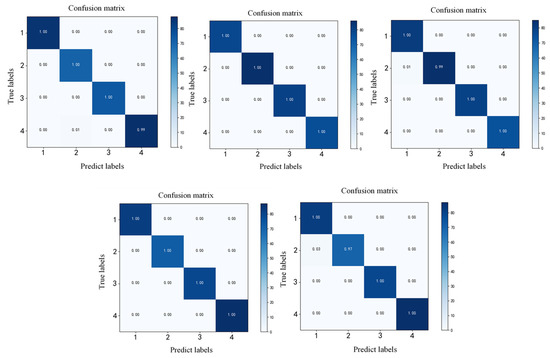
Figure 12.
Defects classification confusion matrix.
According to the characteristics of non-stationary, nonlinear, and vulnerable to noise interference of rail vibration signal, a variable scale non-stationary signal processing method: variational mode decomposition is used. This method can decompose the complex signal into a series of amplitude modulation frequency modulation (AM-FM) signals. The adaptive decomposition of the original signal is realized by using the non-recursive variational mode decomposition model, which can avoid the endpoint effect and suppress modal confusion and has good noise robustness and high decomposition efficiency. VMD decomposition mainly includes under decomposition state and over decomposition state. Under decomposition state refers to the main frequency signal contained in the signal that is not completely decomposed, and over decomposition state refers to those false components are generated in the decomposition process. It can be seen that selecting the appropriate K value can well decompose the frequency components contained in the original signal. In view of this situation, this paper proposes to use the maximum value of envelope kurtosis to determine the optimal mode number of each rail surface defect sample in four channels. Convolutional neural network is widely used in the field of image recognition and has achieved excellent results. It can realize end-to-end learning of image by using basic modules, such as convolutional layer, pooling layer and activation function, avoiding the manual feature extraction of traditional methods.
After VMD decomposition, the signal can reflect the distribution characteristics of the original signal in different frequency bands, which is essentially an enhanced representation of the original signal. By calculating the correlation coefficient between each order eigenmode function of the original signal obtained by variational mode decomposition and the original signal itself, according to its variation law and combined with the filtering characteristics of variational mode decomposition, the eigenmode function with low noise pollution is selected to achieve the purpose of denoising. By encoding the screened multi-sensor components into grayscale images, higher abstract features can be obtained. At the same time, multi-sensor information fusion avoids the experience requirements of experimental personnel for the selection of the optimal sensor position and obtains more comprehensive state features. Thus, the intervention of human experience and knowledge level is reduced, and the accuracy of defects recognition is guaranteed.
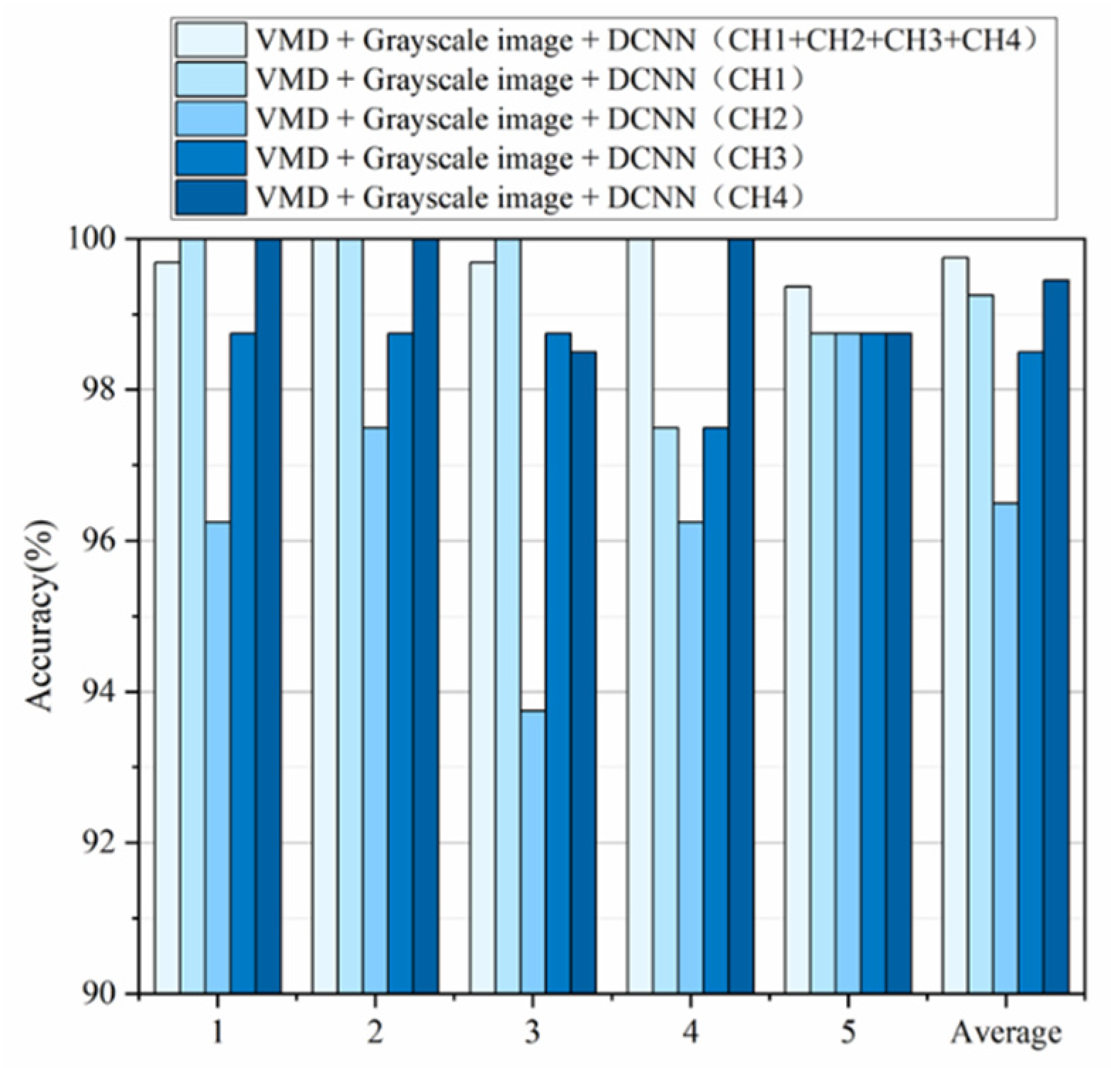
In order to verify the method proposed in this paper, that is, the multi-sensor fusion rail surface defects recognition method based on optimized VMD grayscale image coding and DCNN, which can effectively identify the four rail surface defects of switch, seaming, damage and normal, the following methods are mainly used for comparative analysis: (1) use the signals (four channels) measured by a single sensor to perform VMD to generate grayscale images as the input of DCNN (the DCNN model is the same as that constructed in this paper, only the input is changed), and four groups of comparison results are obtained (the results take the average recognition accuracy of the test set tested for 5 times); (2) MOLO, a new railway surface defect detection method based on end-to-end target detection and lightweight convolution network structure; (3) Rail surface defect detection is realized based on a deep learning algorithm using YOLOv3. Table 9 describes the comparison results of the proposed rail surface defects identification method with four single-sensor as well as MOLO and YOLOv3 comparison methods. Figure 13 shows the comparison between the rail surface defects recognition method proposed in this paper and the results of four single sensors. It can be seen that the multi-sensor fusion rail surface defects recognition method based on VMD grayscale image coding and DCNN proposed in this paper has a higher accuracy.
Table 9.
Performance of different fault diagnosis methods.
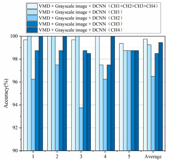
Figure 13.
Comparison results of the first five methods on the same dataset.
3.2. Measured Data Set Result Analysis (Two Categories)
3.2.1. Experimental Data
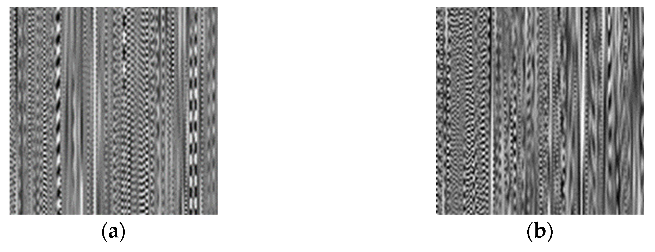
Using the same dataset from the previous section, the data of switch defects, seaming defects, damage defects, and normal states are selected to generate two kinds of grayscale images, normal state, and other state. According to the method proposed in this paper, the measured axle box vibration data set is tested. Figure 14 shows the grayscale images with 128 × 128 pixels.
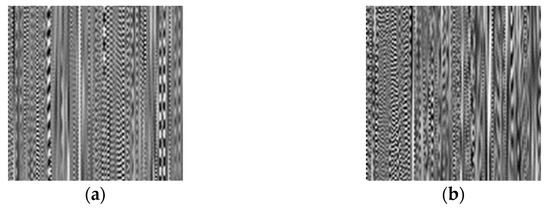
Figure 14.
Example of grayscale image. (a) Normal; (b) Other.
3.2.2. Experimental Result and Analysis
Run the network five times, and Figure 15 shows the identification accuracy and loss rate of the test set obtained from the five tests. Among them, the accuracy changes and loss change curves of the training set and test set in the fourth test are shown in Figure 16.
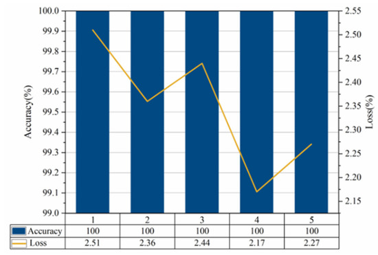
Figure 15.
Accuracy and loss rates for multiple tests.
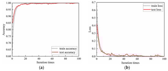
Figure 16.
Accuracy changes and loss changes of training set and test set. (a) Accuracy changes. (b) Loss changes.
Comparing Figure 10 and Figure 16, it can be seen that the proposed multi-sensor fusion rail surface defects recognition method based on VMD grayscale image coding, and DCNN can quickly converge and tend to be stable in both four-class and two-class applications, and the accuracy is higher. It shows that this method has a certain robustness and generality. Five repeated tests results of the classification accuracy of the two categories has reached 100%.
3.3. Anti-Noise Performance Test
3.3.1. Anti-Noise Performance Test Results (Four Categories)
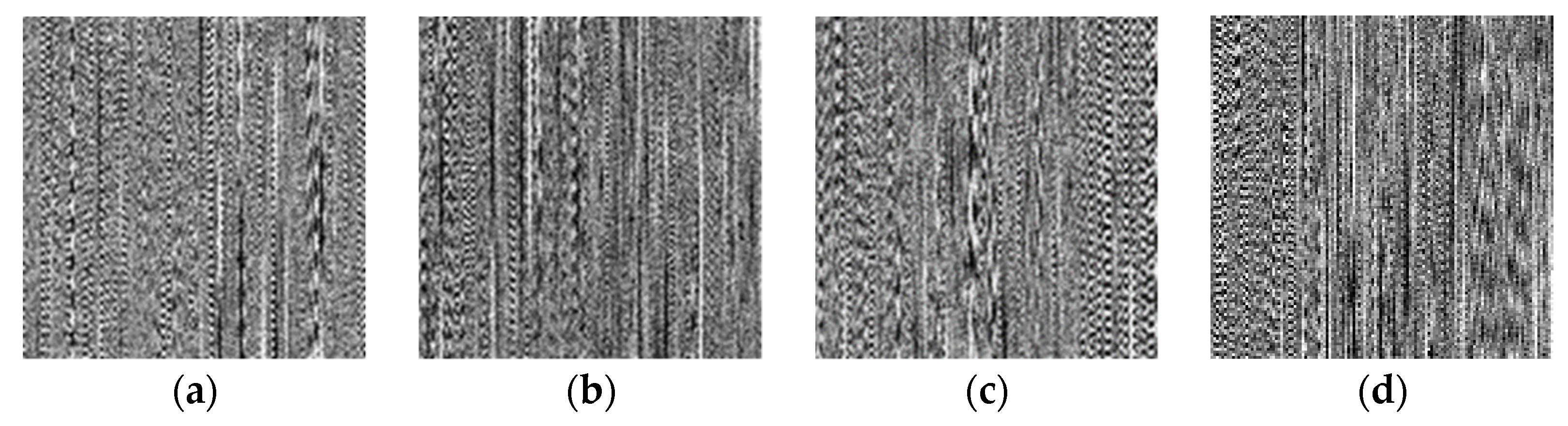
In order to test the anti-noise performance of the method proposed in this paper, 200 noise-added grayscale images with Gaussian noise with variance of 0.01 are added to each of the four rail categories. Figure 17 shows the grayscale images of the four rail categories after adding noise.
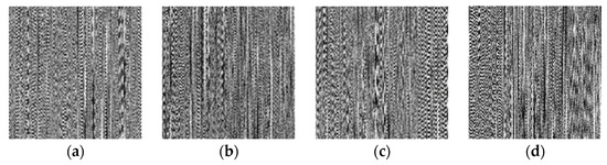
Figure 17.
Grayscale image after adding noise. (a) Switch; (b) Seam; (c) Damage; (d) Normal.
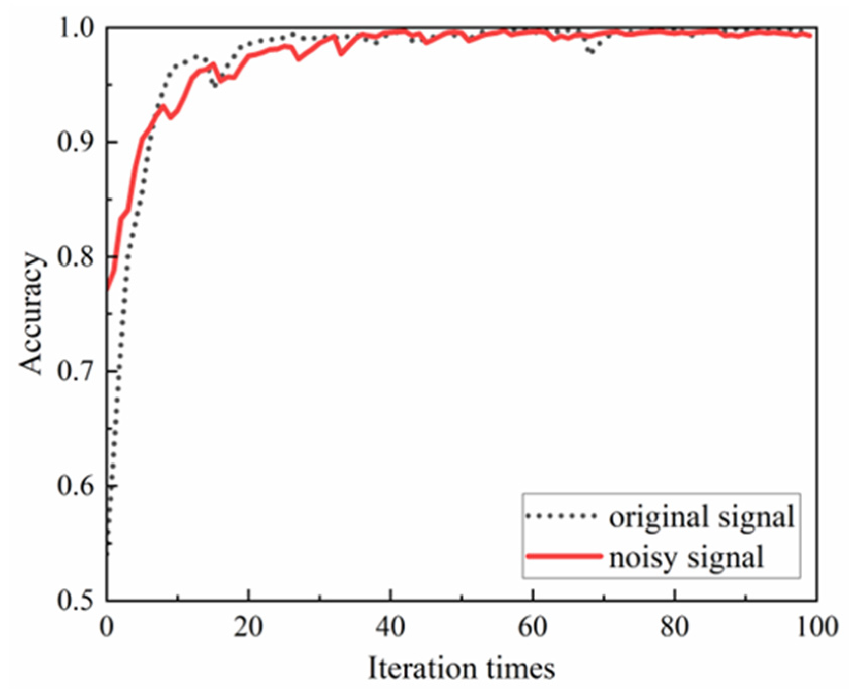
Run the network five times, and Figure 18 shows the recognition accuracy and loss rate of the test set obtained after five cycles of noise adding. Among them, Figure 18 shows the comparison of test set accuracy change curves of the first test results before and after noise addition. It can be seen from Figure 19 that the overall change trend of the two curves is very close. The average accuracy of the final recognition after noise-added is slightly reduced, and the average test accuracy is 99.20%, which is slightly lower than the average test accuracy of the original signal of 99.75%. It shows that the addition of noise image has very little impact on the network, which proves that the DCNN network model proposed in this paper has strong anti-noise ability.
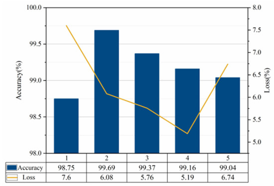
Figure 18.
Accuracy and loss rates for multiple tests.

Figure 19.
Comparison of accuracy change curve of test set before and after noise addition.
3.3.2. Anti-Noise Performance Test Results (Two Categories)
Similarly, in order to test the anti-noise performance of the method proposed in this paper, 200 noise-added grayscale images with Gaussian noise with a variance of 0.01 are added to each of the two rail categories.
The average accuracy of the five repeated tests after noise-added is 99.75%, which is slightly lower than the original tests of 100.00%. It shows that the influence of adding noise image on the network is very small, which proves that the DCNN network model proposed in this paper has strong anti-noise ability.
3.3.3. Discussion
In this sub-section, the accuracy of the identification will be discussed under different rail surface defects. The mixed damage state samples of turnout and damage are separated and used as the fifth rail surface state for diagnosis. That is, the mixed state samples are added to the original turnout, joint, damage and normal state samples, namely, the turnout, joint, damage, turnout and crossing damage, and normal state samples. Only change the sample data set and compare the classification accuracy of four states and five states. The results are shown in the Table 10.
Table 10.
Identification performance of mixed rail surface defects.
It can be seen from the results in the Figure 20 and Table 10 that the classification model trained by the proposed method in this paper can effectively diagnose mixed state samples for the acquired test collection data. In addition, compared with the similar inspection in [19], it only has 34 defect samples, with a prediction accuracy of 88.2%, and a false alarm rate of 10.5%. The accuracy of our model trained by VMD + DCNN network still has the satisfied results.
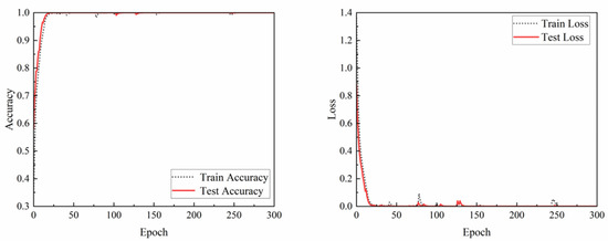
Figure 20.
Comparison of accuracy change curve of test set before and after noise addition.
However, for mixed state samples, the number and diversity of samples needs to be further supplemented. Therefore, the construction of a rail defect identification model based on multi-channel sensing vibration data under mixed state still needs to continue to carry out experiments and in-depth research in future.
4. Conclusions
In order to maximize the use of multi-sensor vibration signals pre-installed in rail vehicles, this paper studies a method to obtain rail surface features by analyzing multi-channel sensor vibration data and construct an effective rail surface defect identification model. Aiming at the characteristics of non-stationary, nonlinear, and easily disturbed by noise of rail vibration signal, and the low recognition rate of some rail surface defects by a single vibration signal, a multi-sensor fusion rail surface defects recognition method based on optimized VMD grayscale image coding and DCNN is proposed. The multi-sensor vibration signal is transformed into grayscale image with obvious characteristics, and the recognition of different rail surface defects types is realized. The main conclusions are as follows:
(1) The parameter-optimized VMD is used to decompose the original vibration acceleration data measured by the four-channel sensors of the axle box, and the IMF component with the largest correlation coefficient between the eigenmode components of each order and the original signal is screened and converted into a grayscale image as the input of DCNN; it avoids the selection of the optimal sensor layout position and reduces the demand for the tester’s actual test experience;
(2) The designed convolution neural network has fast convergence speed and good robustness. The average test accuracy of four classifications and two classifications on the measured data set of on the serviced vehicle reaches 99.75% and 100% respectively, showing good generalization ability. In the anti-noise ability test, the average test accuracy of four classifications and two classifications on the measured data set of on the serviced vehicle is 99.20% and 99.75%, respectively, which reflects the excellent anti-noise ability of the method proposed in this paper;
(3) Under the same conditions, the accuracy of multi-sensor information fusion is 99.75%, which is 0.50%, 3.25%, 1.25%, and 0.30% higher than that of single sensor, indicating that the accuracy of multi-sensor information fusion method is higher than that of single sensor.
Therefore, the proposed optimized VMD grayscale image coding and DCNN can be used for the rail surface defects inspection. In practice, the vibration signals collected from the axle box on the operating service trains can be applied to the proposed method, and the rail surface conditions will be recognized by pre-trained DCNN network models.
In the future, more rail surface images under working conditions will be collected to expand the vibration signal and image database of rail surface defects so as to provide a more powerful guarantee for relevant research work. A variety of rail surface defects are added to verify the universality of the algorithm proposed in this paper. Meanwhile, considering the fusion of rail surface defects image information and vibration signal, a multi-information fusion method more suitable for this research work will be studied [27,28], which gives the rail surface defects image and vibration feature fusion more powerful feature expression ability. In the actual operation of rail transit vehicles, due to noise pollution, such as fog and dust, the visual information will become more blurred and there will be a reduction in the quality of visual information. Further, the efficiency of mounted sensors and the optimized solution will be considered to maintain the multi-sensors fusion to increase the accuracy with fewer sensors.
Author Contributions
S.Z.: conceptualization, project administration, and funding acquisition; Q.Z. and L.P.: methodology, resources, and supervision; X.C.: software, writing—review and editing, and visualization; G.C.: formal analysis, investigation, data curation, and writing—original draft preparation. All authors have read and agreed to the published version of the manuscript.
Funding
This research was supported by the National Natural Science Foundation of China (Grant No. 51975347 and Grant No. 51907117) and Shanghai Science and Technology Program (Grant No. 22010501600).
Data Availability Statement
As the involved project is confidential, Therefore, the data used in this paper is not applicable.
Conflicts of Interest
The authors declare no conflict of interest.
References
- Faghih-Roohi, S.; Hajizadeh, S.; Núñez, A.; Babuska, R.; De Schutter, B. Deep convolutional neural networks for detection of rail surface defects. In Proceedings of the IEEE International Joint Conference on Neural Networks (IJCNN 2016), Vancouver, BC, Canada, 24–29 July 2016. [Google Scholar]
- Yuan, H.; Chen, H.; Liu, S.; Lin, J.; Luo, X. A deep convolutional neural network for detection of rail surface defect. In Proceedings of the IEEE Vehicle Power and Propulsion Conference (VPPC), Hanoi, Vietnam, 14–17 October 2019. [Google Scholar]
- Yu, H.; Li, Q.; Tan, Y.; Gan, J.; Wang, J.; Geng, Y.A.; Jia, L. A coarse-to-fine model for rail surface defect detection. Proc. IEEE Trans. Instrum. Meas. 2018, 68, 656–666. [Google Scholar] [CrossRef]
- Lyu, P.; Zhang, K.; Yu, W.; Wang, B.; Liu, C. A novel RSG-based intelligent bearing fault diagnosis method for motors in high-noise industrial environment. Adv. Eng. Inform. 2022, 52, 101564. [Google Scholar] [CrossRef]
- Chen, J.C.; Chen, T.L.; Liu, W.J.; Cheng, C.C.; Li, M.G. Combining empirical mode decomposition and deep recurrent neural networks for predictive maintenance of lithium-ion battery. Adv. Eng. Inform. 2021, 50, 101405. [Google Scholar] [CrossRef]
- Mićić, M.; Brajović, L.; Lazarević, L.; Popović, Z. Inspection of RCF rail defects—Review of NDT methods. Mech. Syst. Signal Process. 2023, 182, 109568. [Google Scholar] [CrossRef]
- Guo, Y.; Huang, L.; Liu, Y.; Liu, J.; Wang, G. Establishment of the complete closed mesh model of rail-surface scratch data for online repair. Sensors 2020, 20, 4736. [Google Scholar] [CrossRef]
- Zhuang, L.; Wang, L.; Zhang, Z.; Tsui, K.L. Automated vision inspection of rail surface cracks: A double-layer data-driven framework. Transp. Res. Part C Emerg. Technol. 2018, 92, 258–277. [Google Scholar] [CrossRef]
- Jiang, Y.; Wang, H.; Chen, S.; Tian, G. Visual quantitative detection of rail surface crack based on laser ultrasonic technology. Optik 2021, 237, 166732. [Google Scholar] [CrossRef]
- Ramatlo, D.A.; Long, C.S.; Loveday, P.W.; Wilke, D.N. Physics-based modelling and simulation of reverberating reflections in ultrasonic guided wave inspections applied to welded rail tracks. J. Sound Vib. 2022, 530, 116914. [Google Scholar] [CrossRef]
- Liu, Y.; Tian, G.; Gao, B.; Lu, X.; Li, H.; Chen, X.; Zhang, Y.; Xiong, L. Depth quantification of rolling contact fatigue crack using skewness of eddy current pulsed thermography in stationary and scanning modes. NDT E Int. 2022, 128, 102630. [Google Scholar] [CrossRef]
- Kuang, Y.; Chew, Z.J.; Ruan, T.; Lane, T.; Allen, B.; Nayar, B.; Zhu, M. Magnetic field energy harvesting from the traction return current in rail tracks. Appl. Energy 2021, 292, 116911. [Google Scholar] [CrossRef]
- Ma, X.; Wang, P.; Xu, J.; Chen, R. Parameters Studies on Surface Initiated Rolling Contact Fatigue of Turnout Rails by Three-Level Unreplicated Saturated Factorial Design. Appl. Sci. 2018, 8, 461. [Google Scholar] [CrossRef]
- Hamarat, M.; Papaelias, M.; Silvast, M.; Kaewunruen, S. The Effect of Unsupported Sleepers/Bearers on Dynamic Phenomena of a Railway Turnout System under Impact Loads. Appl. Sci. 2020, 7, 2320. [Google Scholar] [CrossRef]
- Yang, H.; Wu, N.; Zhang, W.; Liu, Z.; Fan, J.; Wang, C. Dynamic Response of Spatial Train-Track-Bridge Interaction System Due to Unsupported Track Using Virtual Work Principle. Appl. Sci. 2022, 12, 6156. [Google Scholar] [CrossRef]
- Sysyn, M.; Przybylowicz, M.; Nabochenko, O.; Liu, J. Mechanism of Sleeper–Ballast Dynamic Impact and Residual Settlements Accumulation in Zones with Unsupported Sleepers. Sustainability 2021, 13, 7740. [Google Scholar] [CrossRef]
- Azizi, M.; Shahravi, M.; Zakeri, J.A. Determination of wheel loading reduction in railway track with unsupported sleepers and rail irregularities. Proc. Inst. Mech. Eng. Part F J. Rail Rapid Transit 2021, 235, 631–643. [Google Scholar] [CrossRef]
- Kozhemyachenko, A.A.; And IB, P.; Favorskaya, A.V. Calculation of the stress state of a railway track with unsupported sleepers using the grid-characteristic method. J. Appl. Mech. Tech. Phys. 2021, 62, 344–350. [Google Scholar] [CrossRef]
- Cho, H.; Park, J. Study of Rail Squat Characteristics through Analysis of Train Axle Box Acceleration Frequency. Appl. Sci. 2021, 11, 7022. [Google Scholar] [CrossRef]
- Chang, C.; Ling, L.; Chen, S.; Zhai, W.; Wang, K.; Wang, G. Dynamic performance evaluation of an inspection wagon for urban railway tracks. Measurement 2021, 170, 108704. [Google Scholar] [CrossRef]
- Xiao, Y.; Yan, Y.; Yu, Y.; Wang, B.; Liang, Y. Research on pose adaptive correction method of indoor rail mounted inspection robot in GIS Substation. Energy Rep. 2022, 8, 696–705. [Google Scholar] [CrossRef]
- Sambo, B.; Bevan, A.; Pislaru, C. A novel application of image processing for the detection of rail. In Proceedings of the International Conference on Railway Engineering (ICRE) 2016, Brussels, Belgium, 12–13 May 2016. [Google Scholar]
- Jie, L.; Siwei, L.; Qingyong, L.; Hanqing, Z.; Shengwei, R. Real-time rail head surface defect detection: A geometrical approach. In Proceedings of the IEEE International Symposium on Industrial Electronics, Seoul, Korea, 5–8 July 2009. [Google Scholar]
- Sayeed, M.; Shahin, M.A. Dynamic response analysis of ballasted railway track–ground system under train moving loads using 3D finite element numerical modelling. Transp. Infrastruct. Geotechnol. 2022, 25, 1–21. [Google Scholar] [CrossRef]
- Piao, G.; Li, J.; Udpa, L.; Qian, J.; Deng, Y. Finite-Element Study of Motion-Induced Eddy Current Array Method for High-Speed Rail Defects Detection. IEEE Trans. Magnet. 2021, 57, 6201010. [Google Scholar] [CrossRef]
- Xie, Q.; Tao, G.; He, B.; Wen, Z. Rail corrugation detection using one-dimensional convolution neural network and data-driven method. Measurement 2022, 200, 111624. [Google Scholar] [CrossRef]
- Peng, L.; Zheng, S.; Li, P.; Wang, Y.; Zhong, Q. A Comprehensive Detection System for Track Geometry Using Fused Vision and Inertia. IEEE Trans. Instrum. Meas. 2021, 70, 5004615. [Google Scholar] [CrossRef]
- Peng, L.; Zheng, S.; Zhong, Q.; Chai, X.; Lin, J. A bagged tree ensemble regression method with multiple correlation coefficients to predict the train body vibrations using rail inspection data. Mech. Syst. Signal Process. 2023, 182, 109543. [Google Scholar] [CrossRef]
- Zhang, C.F.; Liu, S.C.; He, J. The Study of Surface State Identification Based on BP_adaboost Algorithm. In Proceedings of the 2018 37th Chinese Control Conference (CCC), Wuhan, China, 25–27 July 2018; pp. 5865–5870. [Google Scholar]
- Ding, J.; Xiao, D.; Li, X. Gear fault diagnosis based on genetic mutation particle swarm optimization VMD and probabilistic neural network algorithm. IEEE Access 2020, 8, 18456–18474. [Google Scholar] [CrossRef]
- Sun, M.; Wang, Y.; Zhang, X.; Liu, Y.; Wei, Q.; Shen, Y.; Feng, N. Feature selection and classification algorithm for non-destructive detecting of high-speed rail defects based on vibration signals. In Proceedings of the 2014 IEEE International Instrumentation and Measurement Technology Conference (I2MTC) Proceedings, Montevideo, Uruguay, 12–15 May 2014; pp. 819–823. [Google Scholar]
- Zhou, Q. A Detection System for Rail Defects Based on Machine Vision. J. Phys. Conf. Ser. 2021, 1748, 022012. [Google Scholar] [CrossRef]
- Liang, B.; Iwnicki, S.; Ball, A.; Young, A.E. Adaptive noise cancelling and time–frequency techniques for rail surface defect detection. Mech. Syst. Signal Process. 2015, 54, 41–51. [Google Scholar] [CrossRef]
- Cheng, H.; Zhang, Y.; Lu, W.; Yang, Z. A bearing fault diagnosis method based on VMD-SVD and Fuzzy clustering. Int. J. Pattern Recognit. Artif. Intell. 2019, 33, 1950018. [Google Scholar] [CrossRef]
- Huang, N.E.; Shen, Z.; Long, S.R.; Wu, M.C.; Shih, H.H.; Zheng, Q.; Liu, H.H. The empirical mode decomposition and the Hilbert spectrum for nonlinear and non-stationary time series analysis. R. Soc. A Math. Phys. Eng. Sci. 1998, 454, 903–995. [Google Scholar] [CrossRef]
- Dragomiretskiy, K.; Zosso, D. Variational mode decomposition. IEEE Trans. Signal Process. 2014, 62, 531–544. [Google Scholar] [CrossRef]
- Li, H.; Liu, T.; Wu, X.; Chen, Q. An optimized VMD method and its applications in bearing fault diagnosis. Measurement 2020, 166, 108185. [Google Scholar] [CrossRef]
- Zhang, X.; Miao, Q.; Zhang, H.; Wang, L. A parameter-adaptive VMD method based on grasshopper optimization algorithm to analyze vibration signals from rotating machinery. Mech. Syst. Signal Process. 2018, 108, 58–72. [Google Scholar] [CrossRef]
- Kowalik, R. Mechanical Wear Contact between the Wheel and Rail on a Turnout with Variable Stiffness. Energies 2021, 14, 7520. [Google Scholar]
- Kisilowski, J.; Kowalik, R. Railroad Turnout Wear Diagnostics. Sensors 2021, 21, 6697. [Google Scholar] [CrossRef]
- Bojarczak, P.; Nowakowski, W. Application of Deep Learning Networks to Segmentation of Surface of Railway Tracks. Sensors 2021, 21, 4065. [Google Scholar] [CrossRef] [PubMed]
- Milosevic, M.D.G.; Pålsson, B.A.; Nissen, A.; Nielsen, J.C.O.; Johansson, H. Condition Monitoring of Railway Crossing Geometry via Measured and Simulated Track Responses. Sensors 2022, 22, 1012. [Google Scholar] [CrossRef]
- Zheng, D.; Li, L.; Zheng, S.; Chai, X.; Zhao, S.; Tong, Q.; Guo, L. A Defect Detection Method for Rail Surface and Fasteners Based on Deep Convolutional Neural Network. Comput. Intell. Neurosci. 2021, 2021, 2565500. [Google Scholar] [CrossRef]
- Chavez-Garcia, R.O.; Aycard, O. Multiple sensor fusion and classification for moving object detection and tracking. IEEE Trans. Intell. Transp. Syst. 2015, 17, 525–534. [Google Scholar] [CrossRef]
- Liang, M.; Yang, B.; Chen, Y.; Hu, R.; Urtasun, R. Multi-task multi-sensor fusion for 3d object detection. In Proceedings of the IEEE/CVF Conference on Computer Vision and Pattern Recognition, Long Beach, CA, USA, 15–20 June 2019; pp. 7345–7353. [Google Scholar]
- Liu, Z.; Cai, Y.; Wang, H.; Chen, L.; Gao, H.; Jia, Y.; Li, Y. Robust target recognition and tracking of self-driving cars with radar and camera information fusion under severe weather conditions. IEEE Trans. Intell. Transp. Syst. 2021, 23, 6640–6653. [Google Scholar] [CrossRef]
- Liu, J.C.; Quan, H.; Yu, X.; He, K.; Li, Z.H. Rolling bearing fault diagnosis based on parameter optimization VMD and sample entropy. Acta Autom. Sin. 2019, 3, 190345. [Google Scholar]
- Gu, R.; Chen, J.; Hong, R.; Wang, H.; Wu, W. Incipient fault diagnosis of rolling bearings based on adaptive variational mode decomposition and Teager energy operator. Measurement 2020, 149, 106941. [Google Scholar] [CrossRef]
- Chen, X.; Lin, J.; Jin, H.; Huang, Y.; Liu, Z. The psychoacoustics annoyance research based on EEG rhythms for passengers in high-speed railway. Appl. Acoust. 2021, 171, 107575. [Google Scholar] [CrossRef]
- Yanan, S.; Hui, Z.; Li, L.; Hang, Z. Rail surface defect detection method based on YOLOv3 deep learning networks. In Proceedings of the 2018 Chinese Automation Congress (CAC), Xi’an, China, 30 November–2 December 2018; pp. 1563–1568. [Google Scholar]
- Lv, J.; Wang, Y.; Ni, P.; Lin, P.; Hou, H.; Ding, J.; Chang, Y.; Hu, J.; Wang, S.; Bao, Z. Development of a high-throughput SNP array for sea cucumber (Apostichopus japonicus) and its application in genomic selection with MCP regularized deep neural networks. Genomics 2022, 114, 110426. [Google Scholar] [CrossRef]
- Hu, X.; Liu, Y.; Zhao, Z.; Liu, J.; Yang, X.; Sun, C.; Chen, S.; Li, B.; Zhou, C. Real-time detection of uneaten feed pellets in underwater images for aquaculture using an improved YOLO-V4 network. Comput. Electron. Agric. 2021, 185, 106135. [Google Scholar] [CrossRef]


Publisher’s Note: MDPI stays neutral with regard to jurisdictional claims in published maps and institutional affiliations. |
© 2022 by the authors. Licensee MDPI, Basel, Switzerland. This article is an open access article distributed under the terms and conditions of the Creative Commons Attribution (CC BY) license (https://creativecommons.org/licenses/by/4.0/).