Article

Hydrodynamic Characteristic-Based Adaptive Model Predictive Control for the Spherical Underwater Robot under Ocean Current Disturbance

1
School of Life Science, Beijing Institute of Technology, Beijing 100081, China
2
Key Laboratory of Convergence Medical Engineering System and Healthcare Technology, Ministry of Industry and Information Technology, School of Life Science, Beijing Institute of Technology, Beijing 100081, China
*
Author to whom correspondence should be addressed.
Machines 2022, 10(9), 798; https://doi.org/10.3390/machines10090798
Submission received: 16 August 2022 / Revised: 6 September 2022 / Accepted: 7 September 2022 / Published: 10 September 2022
(This article belongs to the Special Issue Advances in Underwater Robot Technology)

Abstract

:
In the navigation of underwater robots, large ocean current disturbance often causes significant tracking errors. To better resist ocean current disturbance, the hydrodynamic characteristics of the spherical underwater robot are studied, and a model predictive control strategy based on adaptive model parameters is proposed, according to these characteristics. Firstly, the hydrodynamic characteristics of the robot under static water and constant flow disturbance were obtained and analyzed by the computational fluid dynamics method. Then, the dynamic models of the robot under different disturbances could be calculated from the data obtained, based on the least square method. Finally, an adaptive model predictive control (AMPC) strategy, with an ocean current observer, was designed, based on the dynamic models. When the current disturbance velocity was twice the robot velocity, the proposed strategy reduced the tracking error by 39% and 42% in X and Y directions, respectively. In addition, the hydrodynamic characteristics were verified by experiments.

1. Introduction

With the frequent and deep utilization of resources in the water environment (such as the ocean), various types of underwater robots have been developed, including square, spherical, turtle-shaped, torpedo-shaped, fish-shaped and other bionic robots [1,2,3,4]. Among them, the bionic turtle-shaped robot has the advantages of structural stability and adaptability to underwater exploration [5,6]. The turtle-shaped robots can advance in all directions without rotating the main body, which provides flexibility in turning, rising and sinking [7,8,9]. The bionic robots have a wide range of applications in the fields of marine exploration, marine mapping, cooperative operation, etc. [10,11,12].
After more than 50 years of development, autonomous underwater vehicles (AUVs) have evolved from model building to navigation, control and formation coordination. However, the development of AUVs is still not mature enough. There are still many challenging problems to be solved, including dynamic obstacle avoidance, intelligent formation, and robot control that considers the hydrodynamic effect of complex flow fields. The movement of underwater robots relies on interaction with water. As a result, underwater robots are greatly affected by the currents in the water and are, consequently, more difficult to control in practical applications than robots on roads. AUVs often work in complex flow fields, which makes the dynamic model of AUVs highly nonlinear and strongly coupled. For example, AUVs travel in lakes and oceans with flowing water. In these environments, complex hydrodynamic interactions occur, and the acquisition of data by sensors, and the control of underwater vehicles under unknown hydrodynamic forces, are very difficult and challenging [13,14].
At present, there are three methods to study the hydrodynamic characteristics of robots: test-based methods, predictive methods, and computational fluid dynamics (CFD) methods. The test-based methods provide experimental data for the establishment of vehicular dynamic models, by dragging the robot in a pool or wind tunnel. However, the test-based methods have high costs, due to the corresponding experimental facilities, and it is difficult to implement the methods in some complex environments. In addition, the safety of such methods cannot be guaranteed [15]. Predictive methods aim to obtain hydrodynamic coefficients through theoretical analysis, commonly based on the potential flow theory, such as panel methods and strip methods [16,17]. However, these methods are applicable to typical streamlined cylindrical AUVs, and the modeling error is often large for complex AUVs [18,19]. Computational fluid dynamics (CFD) methods have been widely used to simulate the flow fields, and can also be used in the calculation of dynamic models [20]. The methods use structured or unstructured mesh to discretize the computing domain [21]. CFD technology is economical, and the calculation results are accurate [22,23,24]. The CFD model used in this study adopts the immersed boundary-lattice Boltzmann method (IB-LBM) [25]. Compared with the traditional CFD method, based on finite volume or finite element, this method may easily simulate the movement process of robots in the real situation. Moreover, this method is based on the mesoscopic scale with simple theory, low computation cost and excellent parallelism.
In the process of the robot motion control and trajectory tracking, there are generally two kinds of ways to deal with ocean current disturbance. One is to deal with current disturbance by improving the robustness of the model-free control algorithm [26,27,28]. In addition, the control input can also be compensated by the observed disturbance force through the ocean current observer [29,30,31]. Zhang et al. proposed a dynamic tracking control strategy with fault-tolerant control, and verified that the AUV could realize stable trajectory tracking in a three-dimensional ocean current environment through simulations [32]. Zhou et al. designed a reduced-order extended state observer (RESO) for wave gliders to estimate and compensate for uncertain disturbance, and the performance of the proposed method was verified by simulations and sea trials [33]. The other way to deal with current disturbance is based on model-based control algorithms, such as the model predictive control (MPC) algorithm. The disturbances observed are added to the input of the prediction model (dynamic model) to offset the error caused by the ocean current [34,35]. Dong et al. studied the influence of ocean current disturbance integrated into the kinematic and dynamic model of UMV, and simulations were carried out [36]. However, these studies only considered the influence of disturbance on the input of the prediction model, and did not consider the parameter changes of the prediction model caused by ocean current disturbance [37,38]. These parameters are related to the hydrodynamic characteristics of the robot, and the correlation has been rarely mentioned and explored in previous studies. In early studies, these parameters were generally kept fixed. Some researchers first determined approximate dynamic model parameters in CFD simulation, and then further adjusted these parameters in underwater vehicle experiments [39]. This is a relatively effective method with little disturbance and low requirement for control accuracy. However, with the increasing demand for disturbance resistance, this method cannot meet the requirements of actual scenarios. Therefore, through filtering and machine learning methods, researchers have developed real-time online recognition methods for these parameters. For example, a dynamic model identification method for AUVs, based on factorized Extreme Learning Machine (FELM), has been proposed [40,41]. However, online recognition methods require high computing capability and real-time performance of sensors. This kind of method has a contradiction in terms of the short sampling period but high demand of online calculation. To obtain the changing laws of dynamic model parameters under different disturbances, the analysis and study of hydrodynamic characteristics is necessary. These laws can then be used to solve the uncertainty of model parameters and control stability under ocean current disturbance.
After exploring the hydrodynamic characteristics, the MPC method, based on the kinematic and dynamic model, was chosen. Compared with the traditional Proportion Integration Differentiation (PID) method, the MPC based on the model makes for higher precision of the control, and controllability is stronger in complex environments [42]. In addition, for underwater robot systems, with constraints and strong real-time performance, the MPC method is more suitable for adding constraints and rolling optimization, compared with Linear Quadratic Regulator Control (LQR) and other methods [43]. Therefore, the MPC is widely used in underwater vehicle control and vehicle formation control [44,45,46].
In this paper, the aim was to solve the problem of low control precision and unsteady motion of spherical underwater robots in the presence of constant ocean current disturbance. Firstly, the force and motion of the underwater robot were obtained through CFD simulations, based on the IB-LBM method. Then, the hydrodynamic characteristics of the robot were explored, and the dynamic model of the robot was established, based on the simulation data. With the information acquired, the variations of the dynamic model with disturbance were explored to predict the hydrodynamic coefficients in the dynamic model of the robot. Finally, the kinematic and dynamic models of the robot were used as the reference models of model predictive control (MPC). The adaptive model predictive control (AMPC) strategy, based on adaptive model parameters, and an ocean current observer, based on extended state observer (ESO), were designed to complete the anti-disturbance control of the robot. The correctness of the simulation data was verified by experimental data resulting from experiments in a pool.
The rest of this paper is organized as follows. Section 2 introduces the problem to be solved, the numerical method, and the improved adaptive model predictive control (AMPC). In Section 3, the hydrodynamic characteristics of the robot are analyzed. In Section 4, validation experiments are performed to ensure the correctness of numerical simulations. Based on the Gazebo platform, the tracking performance of the robot using the proposed control strategy is analyzed. Finally, conclusions are presented in Section 5.

2. Modeling and AMPC Strategy

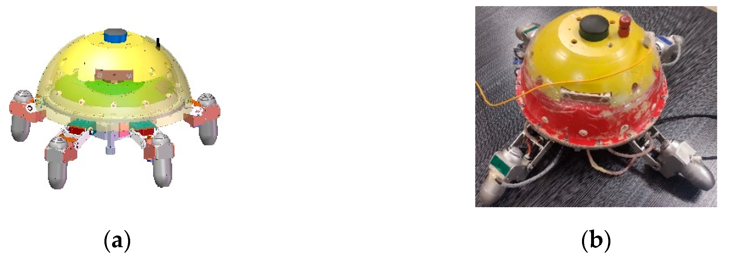
2.1. Problem Description and Numerical Modeling

Amphibious spherical robots have attracted great attention because of their flexible turning and stability. Our study is based on our group’s amphibious spherical robot (ASR-V). Its overall appearance is shown in Figure 1a, and its physical object is shown in Figure 1b. The approximately hemispherical robot body rests on four free legs that may be used for walking on land. In addition, the propeller in each leg allows the robot to swim in all directions under water. This study mainly focused on the underwater movement of the robot. The radius of the ASR-V shell is 0.15 m, and the total weight of this robot is 6.7 kg. The robot is designed to be used in exploration of water environments, including shallow seas, lakes and rivers.
The kinematic and dynamic models of ASR-V are based on the inertial coordinate system and the robot reference coordinate system. The inertial coordinate system O E X E , Y E , Z E is fixed on the earth’s surface and describes the position and attitude of the robot, shown as η = [ x , y , z , ϕ , θ , ψ ] T . The robot reference coordinate system O b x b , y b , z b is fixed on the robot body, generally used to describe the robot’s velocity, and angular velocity, shown as v = [ u , v , w , p , q , r ] T . The origin O b was located in the center of the robot in this study. The linear transformation between the two coordinate systems is expressed as:
η ˙ = J ( η ) v
This is also the kinematic model of the robot. The transformation matrix J ( η ) is expressed as:
J ( η ) = [ J 1 ( η 1 ) 0 3 × 3 0 3 × 3 J 2 ( η 2 ) ]
where, J 1 ( η 1 ) represents the relationship of linear velocity vectors between two coordinate systems, and η 1 = [ x , y , z ] represents the position of the robot. J 2 ( η 2 ) represents the relationship of angular velocity vectors between two coordinate systems, and η 2 = [ ϕ , θ , ψ ] represents the Euler Angle of the robot.
J 1 ( η 1 ) = [ c θ c ψ s θ s ϕ c ψ c ϕ s ψ s ϕ s ψ c ϕ s θ c ψ c θ s ψ s θ s ϕ s ψ + c ϕ c ψ s θ c ϕ s ψ s ϕ c ψ s θ c θ s ϕ c θ c ϕ ]
J 2 ( η 2 ) = [ 1 t θ s ϕ t θ c ϕ 0 c ϕ s ϕ 0 s ϕ / c θ c ϕ / c θ ]  
All parts of the robot used in this paper were rigid, and it was assumed that there was no collision and no elastic deformation on the robot in the movement process. Generally, the dynamic model of the spherical underwater robot is expressed as [47]:
τ = M v ˙ + C ( v ) v + D ( v ) + g ( η ) ,
M = M R B + M A = d i a g { m , m , m , I x , I y , I z } d i a g { X u ˙ , Y v ˙ , Z w ˙ , K p ˙ , M q ˙ , N r ˙ }
C ( v ) = C R B ( v ) + C A ( v )  
D ( v ) = D 1 ( v ) + D 2 ( v ) v
The forces and torques acting on the robot through propulsion equipment is expressed by the vectors τ = [ X , Y , Z , K , M , N ] T and g ( η ) is the restorative force. For ASR, the center of gravity and the center of buoyancy almost coincide, and only the horizontal motion is considered, so the g ( η ) term can be ignored. M R B is the inertia matrix of the rigid body, and M A is the additional mass force matrix. C R B is the rigid body Coriolis-centripetal force matrix, and C A is the additional Coriolis-centripetal force matrix. As C R B , C A and M A are relatively small, they were ignored in this study. D ( v ) is the hydrodynamic damping of the ASR. The D ( v ) and M R B were the main concerns in our study. The dynamic model is simplified into the following form:
τ = M R B v ˙ + ( D 1 ( v ) + D 2 ( v ) v ) v ,
Hydrodynamic damping is coupled and highly nonlinear, especially for underwater robots with complex shapes. Therefore, the variation of hydrodynamic damping coefficients was analyzed under different flow disturbances.
Figure 2 shows the computational domain and grid structure of a simplified robot. The computational domain was 4 m in length, 2 m in width and 1 m in depth. The flow field was filled with a Newtonian fluid at room temperature (20 °C) with a density ρ f = 1.0 × 10 3 kg / m 3 and kinematic viscosity ν f = 1 × 10 6   m 2 / s . The robot model, of the same size and structure as the one in the experiment, was initially stationary in water.
In this study, the fluid simulation was established through the lattice Boltzmann method (LBM), based on the mesoscopic simulation scale [25]. In addition, the immersed boundary method (IBM) was used to deal with moving boundaries, making complex boundary conditions easier to set and calculate [48]. The fluid interaction process described by the IB-LB Method is more efficient [49]. In addition, this method is easy to operate in parallel.
For LBM, the D3Q19 model was used in the flow field. The single relaxation time lattice Boltzmann equation (LBE) is:
f i ( x + c i Δ t , t + Δ t ) = f i ( x , t ) 1 τ [ f i ( x , t ) f i e q ( x , t ) ] + G i ( x , t ) Δ t
In the LBE, f i ( x , t ) is the density distribution function at position x and time t . c i is the discrete velocity for the D3Q19 model, shown as Formula (11). f i e q ( x , t ) represents the equilibrium distribution function shown in Formula (12). G i ( x , t ) is the body force term shown in Formula (13). Δ t is the time step, and τ is the non-dimensional relaxation time:
( c i , i = 0 , , 18 ) = ( c i x c i y c i z ) = c ( 0 0 0   1 0 0   1 0 0   0 1 0   0 1 0   0 0 1   0 0 1   1 1 0   1 1 0   1 1 0   1 1 0   1 0 1   1 0 1   1 0 1   1 0 1   0 1 1   0 1 1   0 1 1   0 1 1 )
f i e q = ω i ρ [ 1 + c i · u c s 2 + ( c i · u ) 2 2 c s 4 u 2 2 c s 2 ] ,
G i ( x , t ) = ( 1 1 2 τ ) ω i [ c i u c s 2 + c i · u c s 4 c i ] · f p ,
In Formula (13), ω i is the weight coefficient. For the D3Q19 model, ω i are given by ω 0 = 1 / 3 , ω 1 6 = 1 / 18 and ω 7 18 = 1 / 36 . f p is the body force acting on the fluid. c s = Δ x / 3 Δ t is the lattice sound speed. The relaxation time τ is related to the kinematic viscosity υ , and it is represented as:
τ = υ c s 2 Δ t + 0.5
The macroscopic fluid density, velocity and pressure are obtained by density distribution functions:
ρ = i f i ,
u = 1 ρ ( i e i f i + 0.5 f p Δ t ) ,
P = i ρ c s 2 .
The edges of the pool were set in accordance with the no slip boundary condition. The complex moving boundaries of the robot body were calculated by the direct force immersion boundary method (IBM). The Lagrangian force density F L ( s , t ) is determined by:
F L = α U u I B Δ t ,
where α is a positive constant. U is the desired velocity obtained by solving the structure dynamics, u I B is the unforced velocity calculated by:
u I B = u ( x , t ) D [ x X ( s , t ) ] d x .
The force of the Lagrange point is dispersed to the Euler point by the following formula:
f ( x , t ) = s F L ( s , t ) D [ x X ( s , t ) ] d s ,
D [ x X ( s , t ) ] is a smoothed approximation of the Dirac delta function.
D ( x ) = 1 h 3 d ( x X h ) d ( y Y h ) d ( z Z h ) ,
d ( r ) = { 1 8 ( 3 2 | r | + 1 + 4 | r | 4 r 2 ) ,             | r | 1 1 8 ( 5 2 | r | 7 + 12 | r | 4 r 2 ) ,       1 | r | 2                         0 ,                                       2 | r | .
The IB-LB Method could simulate the free movement of the robot in the pool model in real time, and obtain the overall force of the robot. In our simulation the grid spacing was Δ x = Δ y = Δ z = 0.1   m in the LBM.

2.2. AMPC with ESO

MPC is a common control algorithm based on the dynamic model. The control process may be optimized in a limited time horizon. In addition, the method can deal with the constraint problem well and make motion control more stable. However, this algorithm depends highly on the model precision. The forces generated by the ocean current in the actual environments are not negligible. At the same time, the dynamic model of the moving robot changes under disturbance, and the control strategy used in static water becomes invalid.
Based on the problem of the uncertain flow disturbance in the actual environment, an AMPC control strategy with an ocean current observer was designed. The ocean current observer was based on the extended state observer (ESO), derived from active disturbance rejection control (ADRC). The ocean current observer has two applications in control decisions. First, observed ocean current disturbance can be added to the controller input as disturbance compensation. Second, the observed ocean current disturbance can modulate the dynamic model parameters, which are the basis for the MPC decisions. The overall control strategy is shown in Figure 3.
The underwater spherical robot belongs to the second order system. The predictive model of MPC is a combination of robot kinematic model and dynamic model.
x ˙ = [ J ( η ) v M 1 ( τ D ( v ) ) ] = f ( x , τ )
x = [ η , v ] , and η = [ x , y ,   z ] is the position information of the robot, v = [ u , w ,   r ] is the speed information of the robot. Taylor expansion is performed at a reference point x d and is subtracted from Formula (23) to obtain the linear state-space model as follows:
x ˜ ˙ = A t ( F d i s ) x ˜ + B t ( F d i s ) τ ˜
where, x ˜ = [ x x d ,   y y d ,   z z d ,   u u d ,   w w d ,   r r d ] , and τ ˜ = [ τ u τ u d ,   τ w τ w d ,   τ r τ r d ] . A t ( F d i s ) and B t ( F d i s ) in state error model (24) are adaptive parameters of the improved MPC, and related to the flow disturbance observed by the extended state observer (ESO). The state-space model is discretized and expanded into the extended state error model:
ξ ( k + 1 ) = A ξ ( k ) + B Δ τ ( k ) ,
η ( k ) = C ξ ( k ) ,
A = [ I + T A t T B t 0 m × n I m ] ,   B = [ T B t I m ] ,   C = [ I n 0 n × m ] ,
where, ξ ( k ) = [ x ˜ ( k ) τ ˜ ( k ) ] , n is the dimension of the state vector and m is the dimension of the control quantity τ . T is the sampling time. According to the mechanical and circuit structure characteristics of the robot, the constraints of control quantity and control increment are considered as Formulae (29) and (30). The model predictive control objective function in this study considered error and control increment. By substituting the predicted output vector, the quadratic optimization problem is as follows:
m i n Δ τ J ( k ) = [ Δ τ ( k ) T , ε ] H ( k ) [ Δ τ ( k ) T , ε ] T + G ( k ) [ Δ τ ( k ) T , ε ] T
s . t .     Δ τ m i n Δ τ ( k ) Δ τ m a x
τ m i n S Δ τ k + 1 N c τ ( k 1 ) τ m a x
H ( k ) is Hessian matrix, which is the coefficient of quadratic optimization problems. The increment of the control input sequence is obtained by solving the above equation.
In 1995, Han Jingqing proposed the ESO, which can be used to observe uncertain disturbance [50]. The ESO was used as the ocean current observer in this paper. The state-space equation of the system after state expansion is:
{ η ˙ = J ( η ) v v ˙ = Γ + M 1 τ Γ ˙ = h y ^ = η
h is the first derivative of the unknown disturbance Γ . Formula (31) can be written as:
{ X ˙ o = A o X o + B o τ + E o h y o = C o X o
where, X o = [ η , v , Γ ] , the matrix A o , B o , C o , E o is easily derived from Formula (31). An observer of lomborg form is constructed for the extended system:
{ X ^ ˙ o = A o X ^ o + B o τ + L ( y o y ^ o ) y ^ o = C o X ^ o
L is the state observer gain matrix. X ^ ˙ o is the state of the system observed and y ^ o is the state observer output. Formula (32) can be subtracted from Formula (33) to obtain:
X ˙ o X ^ ˙ o = ( A L C ) ( X o X ^ o ) + E o h
L is set as L = ( β 1 , β 2 , β 3 ) . The characteristic polynomial of A L C is:
f ( λ ) = λ 2 + β 1 λ 2 + β 2 λ + β 3
By designing the suitable state observer gain matrix L, the extended state observer converges and the disturbance Γ is observed. Then, the corresponding ocean current disturbance is:
F d i s = Γ M 1 D ( v ) v
The adaptive parameters A t ( F d i s ) of the MPC are then be further determined by flow disturbance F d i s .

3. Hydrodynamic Analysis of ASR Robot

The dynamic model of the ASR robot was simplified, based on the following assumptions [51]: (1) The model neglects linear and angular coupled terms. (2) The model assumes that the robot is head–tail and left–right symmetric. (3) Any damping terms greater than second order are neglected. In this section, the hydrodynamic characteristics of the robot are analyzed and discussed through the IB-LB method, focusing on the identification of the relevant hydrodynamic damping coefficients.

3.1. Hydrodynamic Characteristics

The surge motion is the most common mode of underwater movement and defined as the expected forward direction of the robot in this paper. Accordingly, the sway velocity is perpendicular to the surge velocity and conforms to the right-hand rule. The robot may have different deflection angles along the forward direction. The deflection angle of the robot in Figure 4a was set as 0 degrees. Based on this, the hydrodynamic simulations at different angles in expected forward direction without current disturbance were designed, as shown in Figure 4. Then, the curves of the relationship between the surge velocity and the force at different angles were obtained, as shown in Figure 5a.
In Figure 5a, the hydrodynamic damping force on the robot had an approximate quadratic relationship with the surge velocity at the same deflection angle. The damping forces on the robot were also slightly affected by different deflection angles. The detailed relationship between the damping force and the deflection angle is shown in Figure 5b. At the same surge velocity, the damping force increased as the robot deflection angle changed from 0 to 45 degrees. This law was related to the structure of the robot itself.

3.2. Coefficients of Dynamic Model under Different Flow Disturbances

The hydrodynamic damping coefficients of the surge motion were obtained by regression analysis (least squares method) of the computing results in Figure 5. Since the deflection angle of the robot was arbitrary in the process of movement, the average damping forces of 0 and 45 degrees were chosen for the calculation. Through model identification, the relationship between the hydrodynamic damping and the surge velocity without current disturbance could be obtained as follows:
F d i s = 0.0307 u + 28.2862 u 2
It was assumed that the damping coefficients of the robot only contained the velocity and quadratic velocity terms. From the identification formula, the damping of surge motion was mainly linearly related to the quadratic velocity, but less to the first order of velocity.
On the basis of the above hydrodynamic simulations, we obtained the relationship between the damping force and the surge velocity of the robot when the velocity disturbance existed in the sway direction of the robot. The total velocity of the robot, which was relative to the water, were obtained by combining the surge velocity and the disturbance velocity. Then, the total damping force was decomposed to obtain the damping force received in the surge direction of the robot. In Figure 6a, the variation curves of the damping force with the surge velocity at different disturbance velocities (sway velocities) are shown. It can be seen that with increase of disturbance velocities, the damping force in the surge direction became larger, the curvature decreased, and the curve was closer to linear.
Figure 7 shows the influence of the disturbance velocity (sway velocity) on the damping force under different surge velocities. It could be concluded that the greater the surge velocity, the greater the impact of the disturbance velocity. In order to further analyze the influence of disturbance on the damping coefficients, the dynamic model and correlation coefficients were obtained by linear regression analysis. The coefficients of dynamic models under different disturbances are shown in Figure 8. The change of the damping coefficients was nonlinear. In addition, the damping force was more related to the first order of the surge velocity with increase of the disturbance velocity. For example, when the disturbance velocity was 0.3 m/s, the damping force could be expressed as:
F d i s = 7.1857 u + 15.4976 u 2
It could be confirmed by the above analysis that the dynamic model of a robot is difficult to predict without knowing the disturbance velocity, resulting in it being difficult for the control algorithm to be effective under large hydrodynamic disturbances. Therefore, the study of hydrodynamic damping coefficients under disturbance is of great significance to develop better resistance of underwater robots to disturbance and to ensure better movement of the robots in complex current environments.

4. Experimental Evaluation and Discussion

4.1. Validation of Numerical Model

In order to verify the correctness of the numerical simulation method used in this paper, the classical simulation, where water flows around a cylinder, was carried out in a three-dimensional environment. The cylinder diameter D was set as 20 times the lattice length. The flow diagrams near the cylinder under the Reynolds number Re = 40 and Re = 100 were obtained, as shown in Figure 9. Relevant verification parameters were calculated and compared with others’ experimental data, as shown in Table 1. The difference between the simulation results and others’ results was small, which proved the correctness of the simulation method.
Then, we designed a motion process in which the robot achieved uniform speed under fixed thrust for simulations and experiments, as shown in Figure 10. The pool was 2.5 m in length, 1.5 m in width and 0.5 m in depth. In the experiments, the total thrust was kept constant by fixing the speed difference between the front and rear propellers. The dynamometer and the robot were then connected by thin wires to measure the propulsion force of the robot in the water at the same propeller speed. The simulation environment was set according to the pool used in the experiment. In the simulations, the robot was driven by adding propulsion force to the robot body, and, then, the velocity of the robot was measured. The relationship between the velocity and the propulsive force was obtained.
Under the same conditions respectively, four sets of experiments and simulations were carried out to verify the matching of the simulation results with the pool experiments. The comparison between simulation and experimental results is shown in Figure 11. Figure 11a–d correspond to thrust states of 1.37 N, 1.91 N, 2.36 N, and 2.91 N, respectively.
The average velocity errors when the velocity was steady in the four experiments and simulations were 6%, 6%, 15%, and 7%. Through comparison, the rationality and accuracy of the simulation method were verified. The hydrodynamic characteristics of the robot and the dynamic models under disturbance were used in the design of an adaptive model predictive controller, based on the ocean current observer.

4.2. Adaptive Model Predictive Control (AMPC) under Flow Disturbance

According to the analysis in Section 3.2, the damping coefficient of the underwater robot dynamic model varied with different disturbance velocities. The disturbance velocities were observed by the extended state observer (ESO). Then, the AMPC method was carried out by adjusting the parameters of the dynamic model. The simulation scenario is shown in Figure 12. The robot moved underwater, propelled by propellers, with its four legs arranged in an X-shape. An Unmanned Aerial Vehicle (UAV) obtained the position and velocity of the underwater robot through visual recognition, and the data was fed back to the robot for control decisions. In order to verify the performance of the proposed AMPC strategy, three groups of experiments, based on the Gazebo platform, were designed. In each group of experiments, the results of the proposed AMPC strategy with ESO compensation were compared with traditional MPC, traditional MPC with ESO compensation, and AMPC without ESO compensation.
In the first group of experiments, the robot was designed to complete a rectangular trajectory tracking at a speed of 0.1 m/s, and the experimental results are shown in Figure 13 and Figure 14. Figure 13 shows the trajectories of the robot when the disturbance velocity was 0.1 m/s in both X and Y directions. That is, there was flow disturbance of 0.1 ×*√2 m/s in a 45 degrees counterclockwise direction from the X axis. The mean absolute errors of ten experiments are shown in Figure 14. AMPC reduced the mean value of motion error. However, the compensation based ESO introduced large jitter. The reason was that the Gazebo platform was close to the actual physical environment with some unknown unstable factors and disturbance, and recognition errors of UAV also resulted in the jitter of observation and compensation values. In the first group of experiments, the ocean current disturbance was small, and the disturbance force acting on the robot was 0.5486 N. In the second group of experiments, the disturbance velocity was increased to 0.2 m/s in both X and Y directions, with the robot velocity remaining unchanged. The experimental results are shown in Figure 15 and Figure 16.
Figure 15 shows the trajectory of the robot under different control strategies with larger disturbances. Obviously, when the disturbance was large, the traditional MPC could not track the trajectory well. Both ESO and the AMPC strategy could improve the robot’s ability to track the trajectory. In addition, the AMPC strategy combined with ESO, as proposed in this paper, had the best performance. To further illustrate the performance of the proposed method, Figure 16 shows the mean absolute tracking errors of ten experiments in the X and Y directions. Similarly, it could be seen that the AMPC might better reduce the control errors of the robot. After introducing the ESO, the error decreased obviously, but some fluctuations occurred. Overall, in the case of relatively large disturbance, the AMPC with ESO proposed in this paper could better resist disturbance.
In order to further demonstrate the performance of the proposed method, the results of the above two groups of experiments were analyzed quantitatively. The average errors of the whole process when the ocean current disturbance velocities were 0.1 m/s in both the X and Y directions are shown in Table 2. Under this condition, the performance of AMPC without ESO compensation was best, which indicated the effectiveness of the adaptation of the parameters of the models. At the same time, when the ocean disturbance was small, the jitter of the observation value of the ESO made the compensation performance not very significant. ESO, AMPC and their combined algorithms reduced the mean absolute errors of the trajectory tracking by 4%, 16%, and 4% in the X direction, and by 2%, 5%, and 1% in the Y direction, respectively.
Similarly, the average errors of the whole process when the ocean current disturbance velocities were 0.2 m/s in both the X and Y directions are shown in Table 3. With the increase of ocean disturbance velocity, both ESO and AMPC showed good performance against the ocean current disturbance. Under this condition, ESO, AMPC and their combined algorithms reduced the mean absolute errors of the trajectory tracking by 21%, 23%, and 39% in the X direction, and by 23%, 24%, and 42% in the Y direction, respectively.
To verify the effect of the ESO, the calculated observation and compensation values are shown in Figure 17. It can be seen that the observed values fluctuated greatly, and the compensation values obtained by a filter also fluctuated to a certain extent. However, the compensation values were close to the reference values and the errors were small. The errors between the compensation values and the reference values were 0.11 N and 0.16 N. respectively. in the two disturbance environments. The fluctuations of the state observer are unavoidable in a practical environment.
In order to further verify the ability of the proposed control strategy in resisting current disturbance, a third group of experiments were designed. The robot moved in a straight line undergoing a process of acceleration (0–20 s) and then constant velocity (20–50 s) in the X direction. The disturbance velocity was 0.2 m/s in the Y direction. As shown in Figure 18, the mean absolute tracking errors of the robot’s position in the ten experiments are presented. In the acceleration stage, the errors of all methods became larger. The method proposed in this paper had stronger tracking ability and better performance. The average errors of the whole process are shown in Table 4. The experimental results fully demonstrated the anti-disturbance ability of the method proposed in this paper.

5. Conclusions

The navigation of underwater robots is easily influenced by current disturbances and becomes uncontrollable. To solve this problem, the influence of current disturbance on hydrodynamic characteristics and the dynamic model of a robot was investigated, by means of a simplified scenario, in this paper. Then, according to the characteristics of the kinematic and dynamic model with disturbance, AMPC with ESO was proposed. The correctness and performance of this proposed method against disturbance was verified by experiments and simulations. What makes this paper different to most studies, is the fact that the dynamic characteristics of the robot under different current disturbances were applied to the control, and provided a way to resist current disturbance at a lower research cost. In addition, the hydrodynamic characteristics, and the methods of obtaining dynamic models under different disturbances, summarized in this paper may also be applied to robots of other shapes. The exploration of the hydrodynamic characteristics of robots provides reference for future studies of the interaction between robots and underwater currents. In the future, we will consider further exploring the hydrodynamic characteristics of the robot and applying these to control of the robot under time-varying current disturbances.

Author Contributions

Conceptualization, A.L. and S.G.; Data curation, A.L.; Formal analysis, A.L.; Investigation, A.L.; Methodology, A.L.; Project administration, S.G.; Resources, S.G.; Software, A.L.; Supervision, S.G.; Validation, A.L., M.L. and H.Y.; Visualization, A.L.; Writing—original draft, A.L.; Writing—review & editing, A.L., S.G., M.L. and H.Y. All authors have read and agreed to the published version of the manuscript.

Funding

This research received no external funding.

Institutional Review Board Statement

Not applicable.

Informed Consent Statement

Not applicable.

Data Availability Statement

Not applicable.

Conflicts of Interest

The authors declare no conflict of interest.

References

  1. Xing, H.; Shi, L.; Hou, X.; Liu, Y.; Hu, Y.; Xia, D.; Li, Z.; Guo, S. Design, Modeling and Control of a Miniature Bio-Inspired Amphibious Spherical Robot. Mechatronics 2021, 77, 102574. [Google Scholar] [CrossRef]
  2. Katzschmann, R.K.; DelPreto, J.; MacCurdy, R.; Rus, D. Exploration of Underwater Life with an Acoustically Controlled Soft Robotic Fish. Sci. Robot. 2018, 3, eaar3449. [Google Scholar] [CrossRef]
  3. Costa, D.; Palmieri, G.; Palpacelli, M.-C.; Panebianco, L.; Scaradozzi, D. Design of a Bio-Inspired Autonomous Underwater Robot. J. Intell. Robot. Syst. 2018, 91, 181–192. [Google Scholar] [CrossRef]
  4. Honaryar, A.; Ghiasi, M. Design of a Bio-Inspired Hull Shape for an AUV from Hydrodynamic Stability Point of View through Experiment and Numerical Analysis. J. Bionic Eng. 2018, 15, 950–959. [Google Scholar] [CrossRef]
  5. Chemori, A.; Kuusmik, K.; Salumäe, T.; Kruusmaa, M. Depth Control of the Biomimetic U-CAT Turtle-Like AUV with Experiments in Real Operating Conditions. In Proceedings of the 2016 IEEE International Conference on Robotics and Automation (ICRA), Stockholm, Sweden, 16–21 May 2016. [Google Scholar]
  6. Guo, J.; Li, C.; Guo, S. A Novel Step Optimal Path Planning Algorithm for the Spherical Mobile Robot Based on Fuzzy Control. IEEE Access 2020, 8, 1394–1405. [Google Scholar] [CrossRef]
  7. Guo, J.; Li, C.; Guo, S. Study on the Autonomous Multirobot Collaborative Control System Based on Spherical Amphibious Robots. IEEE Syst. J. 2021, 15, 4950–4957. [Google Scholar] [CrossRef]
  8. Hou, X.; Li, Z.; Guo, S.; Shi, L.; Xing, H.; Yin, H. An Improved Backstepping Controller with an LESO and TDs for Robust Underwater 3D Trajectory Tracking of a Turtle-Inspired Amphibious Spherical Robot. Machines 2022, 10, 450. [Google Scholar] [CrossRef]
  9. Allotta, B.; Costanzi, R.; Pugi, L.; Ridolfi, A. Identification of the Main Hydrodynamic Parameters of Typhoon AUV from a Reduced Experimental Dataset. Ocean Eng. 2018, 147, 77–88. [Google Scholar] [CrossRef]
  10. Li, C.; Guo, S.; Guo, J. Performance Evaluation of a Hybrid Thruster for Spherical Underwater Robots. IEEE Trans. Instrum. Meas. 2022, 71, 7503110. [Google Scholar] [CrossRef]
  11. Xing, H.; Liu, Y.; Guo, S.; Shi, L.; Hou, X.; Liu, W.; Zhao, Y. A Multi-Sensor Fusion Self-Localization System of a Miniature Underwater Robot in Structured and GPS-Denied Environments. IEEE Sens. J. 2021, 21, 27136–27146. [Google Scholar] [CrossRef]
  12. An, R.; Guo, S.; Yu, Y.; Li, C.; Awa, T. Multiple Bio-Inspired Father-Son Underwater Robot for Underwater Target Object Acquisition and Identification. Micromachines 2022, 13, 25. [Google Scholar] [CrossRef]
  13. Mitra, A.; Panda, J.P.; Warrior, V.H. Experimental and Numerical Investigation of the Hydrodynamic Characteristics of Autonomous Underwater Vehicles over Sea-Beds with Complex Topography. Ocean Eng. 2020, 198, 106978. [Google Scholar] [CrossRef]
  14. Panda, J.P.; Mitra, A.; Warrior, V.H. A Review on the Hydrodynamic Characteristics of Autonomous Underwater Vehicles. Proc. Inst. Mech. Eng. Part M-J. Eng. Marit. Environ. 2021, 235, 15–29. [Google Scholar] [CrossRef]
  15. Guo, S.; He, Y.; Shi, L.; Pan, S.; Xiao, R.; Tang, K.; Guo, P. Modeling and Experimental Evaluation of an Improved Amphibious Robot with Compact Structure. Robot. Comput. Integr. Manuf. 2018, 51, 37–52. [Google Scholar] [CrossRef]
  16. Milgram, J.H. Strip Theory for Underwater Vehicles in Water of Finite Depth. J. Eng. Math. 2007, 58, 31–50. [Google Scholar] [CrossRef]
  17. Gu, S.; Guo, S. Performance Evaluation of a Novel Propulsion System for the Spherical Underwater Robot (SURIII). Appl. Sci. 2017, 7, 1196. [Google Scholar] [CrossRef]
  18. Porez, M.; Boyer, F.; Ijspeert, A.J. Improved Lighthill Fish Swimming Model for Bio-Inspired Robots: Modeling, Computational Aspects and Experimental Comparisons. Int. J. Robot. Res. 2014, 33, 1322–1341. [Google Scholar] [CrossRef]
  19. Gu, S.; Guo, S.; Zheng, L. A Highly Stable and Efficient Spherical Underwater Robot with Hybrid Propulsion Devices. Auton. Robots 2020, 44, 759–771. [Google Scholar] [CrossRef]
  20. Hou, X.; Guo, S.; Shi, L.; Xing, H.; Liu, Y.; Liu, H.; Hu, Y.; Xia, D.; Li, Z. Hydrodynamic Analysis-Based Modeling and Experimental Verification of a New Water-Jet Thruster for an Amphibious Spherical Robot. Sensors 2019, 19, 259. [Google Scholar] [CrossRef]
  21. Mostafapour, K.; Nouri, N.M.; Zeinali, M. The Effects of the Reynolds Number on the Hydrodynamics Characteristics of an AUV. J. Appl. Fluid Mech. 2018, 11, 343–352. [Google Scholar] [CrossRef]
  22. Zhang, B.; Lu, X.; She, W. Resistance Performance Simulation of Remotely Operated Vehicle in Deep Sea Considering Propeller Rotation. Proc. Inst. Mech. Eng. Part M-J. Eng. Marit. Environ. 2020, 234, 585–598. [Google Scholar] [CrossRef]
  23. Saghafi, M.; Lavimi, R. Optimal Design of Nose and Tail of an Autonomous Underwater Vehicle Hull to Reduce Drag Force Using Numerical Simulation. Proc. Inst. Mech. Eng. Part M-J. Eng. Marit. Environ. 2020, 234, 76–88. [Google Scholar] [CrossRef]
  24. Anbarsooz, M. A Numerical Study on Drag Reduction of Underwater Vehicles Using Hydrophobic Surfaces. Proc. Inst. Mech. Eng. Part M-J. Eng. Marit. Environ. 2019, 233, 301–309. [Google Scholar] [CrossRef]
  25. Zhang, Y.; Pan, G.; Zhang, Y.; Haeri, S. A Relaxed Multi-Direct-Forcing Immersed Boundary-Cascaded Lattice Boltzmann Method Accelerated on GPU. Comput. Phys. Commun. 2020, 248, 106980. [Google Scholar] [CrossRef]
  26. Meng, C.; Zhang, X. Distributed Leaderless Formation Control for Multiple Autonomous Underwater Vehicles Based on Adaptive Nonsingular Terminal Sliding Mode. Appl. Ocean. Res. 2021, 115, 102781. [Google Scholar] [CrossRef]
  27. Vu, M.T.; Le Thanh, H.N.N.; Huynh, T.-T.; Do, Q.T.; Do, T.D.; Hoang, Q.-D.; Le, T.-H. Station-Keeping Control of a Hovering over-Actuated Autonomous Underwater Vehicle under Ocean Current Effects and Model Uncertainties in Horizontal Plane. IEEE Access 2021, 9, 6855–6867. [Google Scholar] [CrossRef]
  28. Wu, H.-M.; Karkoub, M. Finite-Time Robust Tracking Control of an Autonomous Underwater Vehicle in the Presence of Uncertainties and External Current Disturbances. Adv. Mech. Eng. 2021, 13, 16878140211053429. [Google Scholar] [CrossRef]
  29. Wang, H.; Dong, J.; Liu, Z.; Yan, L.; Wang, S. Control Algorithm for Trajectory Tracking of an Underactuated USV under Multiple Constraints. Math. Probl. Eng. 2022, 2022, 5274452. [Google Scholar] [CrossRef]
  30. Wei, H.; Shen, C.; Shi, Y. Distributed Lyapunov-Based Model Predictive Formation Tracking Control for Autonomous Underwater Vehicles Subject to Disturbances. IEEE Trans. Syst. Man Cybern. 2021, 51, 5198–5208. [Google Scholar] [CrossRef]
  31. Mu, W.; Wang, Y.; Sun, H.; Liu, G. Double-Loop Sliding Mode Controller with an Ocean Current Observer for the Trajectory Tracking of ROV. J. Mar. Sci. Eng. 2021, 9, 1000. [Google Scholar] [CrossRef]
  32. Zhang, H.; Zhu, D.; Liu, C.; Hu, Z. Tracking Fault-Tolerant Control Based on Model Predictive Control for Human Occupied Vehicle in Three-Dimensional Underwater Workspace. Ocean Eng. 2022, 249, 110845. [Google Scholar] [CrossRef]
  33. Zhou, Y.; Sun, X.; Sang, H.; Yu, P. Robust Dynamic Heading Tracking Control for Wave Gliders. Ocean Eng. 2022, 256, 111510. [Google Scholar] [CrossRef]
  34. Vu, M.T.; Le, T.-H.; Thanh, H.L.N.N.; Huynh, T.-T.; Van, M.; Hoang, Q.-D.; Do, T.D. Robust Position Control of an over-Actuated Underwater Vehicle under Model Uncertainties and Ocean Current Effects Using Dynamic Sliding Mode Surface and Optimal Allocation Control. Sensors 2021, 21, 747. [Google Scholar] [CrossRef]
  35. Miao, J.; Wang, S.; Tomovic, M.M.; Zhao, Z. Compound Line-of-Sight Nonlinear Path Following Control of Underactuated Marine Vehicles Exposed to Wind, Waves, and Ocean Currents. Nonlinear Dyn. 2017, 89, 2441–2459. [Google Scholar] [CrossRef]
  36. Dong, Z.; Wan, L.; Liu, T.; Zeng, J. Horizontal-Plane Trajectory-Tracking Control of an Underactuated Unmanned Marine Vehicle in the Presence of Ocean Currents. Int. J. Adv. Robot. Syst. 2016, 13, 83. [Google Scholar] [CrossRef]
  37. Gibson, S.B.; Stilwell, D.J. Hydrodynamic Parameter Estimation for Autonomous Underwater Vehicles. IEEE J. Ocean. Eng. 2020, 45, 385–394. [Google Scholar] [CrossRef]
  38. Mirzaei, M.; Taghvaei, H. A Full Hydrodynamic Consideration in Control System Performance Analysis for an Autonomous Underwater Vehicle. J. Intell. Robot. Syst. 2020, 99, 129–145. [Google Scholar] [CrossRef]
  39. Alam, K.; Ray, T.; Anavatti, S.G. Design Optimization of an Unmanned Underwater Vehicle Using Low- and High-Fidelity Models. IEEE Trans. Syst. Man Cybern. 2017, 47, 2794–2808. [Google Scholar] [CrossRef]
  40. Rath, B.N.; Subudhi, B. A Robust Model Predictive Path Following Controller for an Autonomous Underwater Vehicle. Ocean Eng. 2022, 244, 110265. [Google Scholar] [CrossRef]
  41. Bibuli, M.; Zereik, E.; De Palma, D.; Ingrosso, R.; Indiveri, G. Analysis of an Unmanned Underwater Vehicle Propulsion Model for Motion Control. J. Guid. Control. Dyn. 2022, 45, 1046–1059. [Google Scholar] [CrossRef]
  42. Barjuei, E.S.; Gasparetto, A. Predictive Control of Spatial Flexible Mechanisms. Int. J. Mech. Control 2015, 16, 85–96. [Google Scholar]
  43. Prasad, M.P.R.; Swarup, A. Position and Velocity Control of Remotely Operated Underwater Vehicle Using Model Predictive Control. Indian J. Geo-Mar. Sci. 2015, 44, 1920–1927. [Google Scholar]
  44. Hou, X.; Guo, S.; Shi, L.; Xing, H.; Yin, H.; Li, Z.; Zhou, M.; Xia, D. Improved Model Predictive-Based Underwater Trajectory Tracking Control for the Biomimetic Spherical Robot under Constraints. Appl. Sci. 2020, 10, 8106. [Google Scholar] [CrossRef]
  45. Chu, Z.; Wang, D.; Meng, F. An Adaptive RBF-NMPC Architecture for Trajectory Tracking Control of Underwater Vehicles. Machines 2021, 9, 105. [Google Scholar] [CrossRef]
  46. Shen, C.; Shi, Y.; Buckham, B. Path-Following Control of an AUV: A Multiobjective Model Predictive Control Approach. IEEE Trans. Control Syst. Technol. 2019, 27, 1334–1342. [Google Scholar] [CrossRef]
  47. Gao, J.; Liang, X.; Chen, Y.; Zhang, L.; Jia, S. Hierarchical Image-Based Visual Serving of Underwater Vehicle Manipulator Systems Based on Model Predictive Control and Active Disturbance Rejection Control. Ocean Eng. 2021, 229, 108814. [Google Scholar] [CrossRef]
  48. Li, A.; Xu, G.-M.; Ma, J.-T.; Xu, Y.-Q. Study on the Binding Focusing State of Particles in Inertial Migration. Appl. Math. Model. 2021, 97, 1–18. [Google Scholar] [CrossRef]
  49. Xu, Y.-Q.; Wang, M.-Y.; Liu, Q.-Y.; Tang, X.-Y.; Tian, F.-B. External Force-Induced Focus Pattern of a Flexible Filament in a Viscous Fluid. Appl. Math. Model. 2018, 53, 369–383. [Google Scholar] [CrossRef]
  50. Zhou, W.; Guo, S.; Guo, J.; Meng, F.; Chen, Z. ADRC-Based Control Method for the Vascular Intervention Master-Slave Surgical Robotic System. Micromachines 2021, 12, 1439. [Google Scholar] [CrossRef]
  51. Lamas, I.M.; Rodriguez, C.G. Hydrodynamics of Biomimetic Marine Propulsion and Trends in Computational Simulations. J. Mar. Sci. Eng. 2020, 8, 479. [Google Scholar] [CrossRef]
  52. Russell, D.; Wang, Z.J. A Cartesian Grid Method for Modeling Multiple Moving Objects in 2D Incompressible Viscous Flow. J. Comput. Phys. 2003, 191, 177–205. [Google Scholar] [CrossRef]
  53. Linnick, M.N.; Fasel, H.F. A High-Order Immersed Interface Method for Simulating Unsteady Incompressible Flows on Irregular Domains. J. Comput. Phys. 2005, 204, 157–192. [Google Scholar] [CrossRef]
  54. Hu, Y.; Yuan, H.; Shu, S.; Niu, X.; Li, M. An Improved Momentum Exchanged-Based Immersed Boundary-Lattice Boltzmann Method by Using an Iterative Technique. Comput. Math. Appl. 2014, 68, 140–155. [Google Scholar] [CrossRef]
Figure 1. The model structure of the amphibious spherical robot (ASR). (a) The overall appearance of the ASR-V robot; (b) The physical object of the ASR-V robot.
Machines 10 00798 g001
Figure 2. The computational fluid dynamic model used to simulate the actual physics experiments based on the immersed boundary-lattice Boltzmann method (IB-LBM). (a) The computational domain; (b) The simplified model of the robot.
Machines 10 00798 g002
Figure 3. The adaptive model predictive control (AMPC) control strategy with ocean current observer.
Machines 10 00798 g003
Figure 4. The schematic diagram of hydrodynamic simulations at different angles. (a) radian = 0   rad ; (b) radian = 0.2618   rad ; (c) radian = 0.5236   rad ; (d) radian = 0.7854   rad .
Machines 10 00798 g004
Figure 5. The relationships between damping force, surge velocity and deflection angle in surge direction. (a) Damping force–surge velocity; (b) Damping force–deflection angle.
Machines 10 00798 g005
Figure 6. The damping force characteristics under disturbance. (a) The damping force changing with surge velocity under different disturbance velocities; (b) The three-dimensional curve relating the damping force, surge velocity and the disturbance velocity (sway velocity).
Machines 10 00798 g006
Figure 7. The curve of damping force in surge direction changing with disturbance velocity (sway velocity) under different surge velocities.
Machines 10 00798 g007
Figure 8. The relation between the damping coefficients of surge motion and the disturbance velocity in sway direction.
Machines 10 00798 g008
Figure 9. The flow field and streamline around a cylinder. (a) Re = 40; (b) Re = 100.
Machines 10 00798 g009
Figure 10. Experiment and simulation scenes. The black arrows represent the direction of the robot moving. (a) The propulsion force measurement; (b) The robot moving under water; (c) The simulation.
Machines 10 00798 g010
Figure 11. The comparison of experiments and simulations on force–velocity relationships. (a) Thrust 0.37 N; (b) Thrust 0.91 N; (c) Thrust 1.36 N; (d) Thrust 1.91 N.
Machines 10 00798 g011
Figure 12. The simulation scenario of underwater robot tracking on the Gazebo platform. (a) Top view; (b) Elevation view.
Machines 10 00798 g012
Figure 13. The trajectory of the robot when the disturbance velocities were u = 0.1 m/s and v = 0.1 m/s. (a) The overall trajectory; (b) The trajectory from −3 m to 2 m in the X direction; (c) The trajectory from −3 m to 2 m in the Y direction; (d) The trajectory from 2 m to −3 m in the X direction; (e) The trajectory from 2 m to −3 m in the Y direction.
Machines 10 00798 g013aMachines 10 00798 g013b
Figure 14. The position error of the robot at the disturbance velocities u = 0.1 m/s and v = 0.1 m/s. (a) The trajectory error in the X direction; (b) The trajectory error in the Y direction.
Machines 10 00798 g014
Figure 15. The trajectory of the robot when the disturbance velocities were u = 0.2 m/s and v = 0.2 m/s. (a) The diagram of the overall trajectory; (b) The trajectory from −3 m to 2 m in the X direction; (c) The trajectory from −3 m to 2 m in the Y direction; (d) The trajectory from 2 m to −3 m in the X direction; (e) The trajectory from 2 m to −3 m in the Y direction.
Machines 10 00798 g015aMachines 10 00798 g015b
Figure 16. The position error of the robot at the disturbance velocities u = 0.2 m/s and v = 0.2 m/s. (a) The trajectory error in the X direction; (b) The trajectory error in the Y direction.
Machines 10 00798 g016
Figure 17. The observed values of the extended state observer (ESO) under two different velocity disturbances. (a) Observer at u = 0.1 m/s, v = 0.1 m/s; (b) Observer at u = 0.2 m/s, v = 0.2 m/s.
Machines 10 00798 g017
Figure 18. The simulation results for robot trajectory tracking. (a) The trajectory error in the X direction; (b) The trajectory error in the Y direction.
Machines 10 00798 g018
Table 1. Comparison of related parameters in flow around cylinder.
Re40 100
CdLw/DCdClSt
Russell [52]1.602.291.430.3220.172
Linnick [53]1.542.281.380.3370.169
Hu [54]1.662.551.480.3670.166
Present1.601.601.440.3410.157
Table 2. The average errors of the whole process with 0.1 m/s disturbance velocities in both the X and Y directions.
Mean ErrorTraditional MPCMPC + ESOMPC + AdaptionMPC + ESO + Adaption
X direction (m)0.1480.1410.1240.141
Y direction (m)0.1290.1260.1220.128
Table 3. The average errors of the whole process with 0.2 m/s disturbance velocities in both the X and Y directions.
Mean ErrorTraditional MPCMPC + ESOMPC + AdaptionMPC + ESO + Adaption
X direction (m)0.2790.2200.2150.169
Y direction (m)0.2510.1940.1910.146
Table 4. The average errors of the whole process with 0.2 m/s disturbance velocities in the Y direction.
Mean ErrorTraditional MPCMPC + ESOMPC + AdaptionMPC + ESO + Adaption
X direction (m)0.3020.2730.2500.235
Y direction (m)0.2580.1200.1330.056
Publisher’s Note: MDPI stays neutral with regard to jurisdictional claims in published maps and institutional affiliations.

