The Graph Neural Network Detector Based on Neighbor Feature Alignment Mechanism in LIDAR Point Clouds

Abstract

Three-dimensional (3D) object detection has a vital effect on the environmental awareness task of autonomous driving scenarios. At present, the accuracy of 3D object detection has significant improvement potential. In addition, a 3D point cloud is not uniformly distributed on a regular grid because of its disorder, dispersion, and sparseness. The strategy of the convolution neural networks (CNNs) for 3D point cloud feature extraction has the limitations of potential information loss and empty operation. Therefore, we propose a graph neural network (GNN) detector based on neighbor feature alignment mechanism for 3D object detection in LiDAR point clouds. This method exploits the structural information of graphs, and it aggregates the neighbor and edge features to update the state of vertices during the iteration process. This method enables the reduction of the offset error of the vertices, and ensures the invariance of the point cloud in the spatial domain. For experiments performed on the KITTI public benchmark, the results demonstrate that the proposed method achieves competitive experimental results.

1. Introduction

Three-dimensional (3D) object detection has a vital effect on the environmental awareness task of autonomous driving scenarios. It is a critical technology to identify and predict potential dangers, which ensures the safety of vehicles and pedestrians on the driving road. The purpose of 3D object detection is to discover important information about the object in the driving scenario, such as 3D coordinates, length, width, height, and rotation angle of the horizontal plane. At present, the accuracy of 3D object detection has significant improvement potential. The existing methods utilize various data forms for 3D object detection, which include monocular vision [1], stereo vision [2], RGB-D images [3], and point clouds [4].

Compared with monocular and stereo vision methods with RGB images, the point cloud has a more robust performance. Point cloud data enable the decoupling of objects and backgrounds, which is more conducive to information mining. In particular, point clouds could provide very accurate 3D coordinate information in foggy or night scenes, while, with RGB images, it is difficult to determine coordinate positions by pixel information in these scenes. A common information data format in autonomous driving scenarios is the 3D point cloud obtained from LiDAR sensors, which assist autonomous vehicles in obtaining accurate predictions. Therefore, this work utilizes the LiDAR point cloud as input data for the study of 3D object detection.

Three-dimensional point cloud data are not uniformly distributed on a regular grid because of their disorder, dispersion, and sparseness. The strategy of the regular grid for 3D point cloud feature extraction has the limitations of potential information loss and empty operation [4]. Therefore, the 3D point cloud is converted into a graph representation for model training in this work. However, it may contain the problem that a non-fixed number of neighbors and the feature information of edges are not used effectively when processing with convolution operation in the graph representation structure. To address the aforementioned limitations of convolutional neural networks in 3D point clouds, some methods have transformed sparse point clouds into compactly shaped three-dimensional representations by using voxelization [5,6], while others have performed 3D object detection by directly processing point clouds [7,8].

However, the two mentioned methods remain computationally challenging. Therefore, this work considers utilizing the graph neural network (GNN) [9] instead of the convolutional neural network (CNN) [10] for 3D object detection. Multilayer Perceptrons (MLPs) are used to handle some disordered property problems [11]. In addition, the amount of 3D point cloud provided by LiDAR is comparatively heavy, which generates a large computational cost in model detection. To improve the processing speed of the model, voxelization strategies are used in some methods to reduce the density of the point cloud [6]. However, the voxelization strategy used in the above method requires sampling a fixed number of points for each voxel, which results in extra capacity and computational cost. Moreover, this method affects by the random drop operation, which might result in unstable detection results in the model.

In summary, we propose a graph neural network framework based on neighbor feature alignment mechanism for 3D object detection in LiDAR point clouds. The neighbor feature represents the vertices in the graph that have a connection relationship with the centroid. The proposed method retains the richer feature information of the point cloud by constructing a graph. Considering that LiDAR point clouds have a large amount of data, we propose a dynamic sparsification method for reducing the point cloud density. Secondly, aiming to effectively utilize the vertex and edge feature information in the graph, we propose a neighbor feature alignment mechanism for feature extraction. The experiments on the public benchmark KITTI dataset demonstrate that the proposed method achieves a competitive detection performance.

The main contributions of this paper are as follows:

(1)

We propose a novel graph neural network framework based on neighbor feature alignment mechanism for 3D object detection. This framework converts the input point cloud into a graph and uses a graph neural network for feature extraction, which implements the 3D object detection in LiDAR point clouds.

(2)

A neighbor feature alignment mechanism is proposed. This method exploits the structural information of graph, and it aggregates the neighbor and edge features to update the state of vertices during the iteration process. This method enables the reduction of the offset error of the vertices, and ensures the invariance of the point cloud in the spatial domain.

(3)

We conduct extensive experiments on the public benchmark KITTI dataset for autonomous driving. The experiments demonstrate that the proposed method achieves competitive experimental results.

2. Related Works

LiDAR is an indispensable sensor in unmanned systems, which could provide the dense 3D point cloud for accurately representing the shape and location of the object in 3D space. Therefore, the environment perception algorithm based on LiDAR point cloud has become an emphasis of current research in unmanned systems. The object detection algorithms based on LiDAR point clouds can be categorized as multi-view-based methods, voxel-based methods, point-based methods, and the combined point-voxel methods.

The voxel-based methods. VoxelNet [6] has quantified the point clouds into grid data, which can automatically learn usable information from the point clouds in an end-to-end process, being more efficient than the manual way of designing features. The main problem of this method is that the intermediate layer adopted the 3D convolution, which has excessive computation resulting in the operation speed not satisfying the real-time requirement. SECOND [12] adopted a sparse convolution strategy to avoid invalid computation in the empty region, which improved the operation speed and reduced the usage of the graphics memory at the same time. CIA-SSD [13] also adopted 3D sparse convolution for feature extraction. The difference is that CIA-SSD took the mean value of the points in the grid as the starting features, further reduced the computational effort by continuously decreasing the spatial resolution, and finally stitched the features in the Z-direction to obtain a 2D feature map. PIXOR [4] proposed a manual design to compress the 3D Voxel to 2D Pixel. This method avoided the problem of excessive computation by using 3D convolution, but the information in the height direction was lost, which resulted in a decrease in detection accuracy. PointPillar [14] also adopted the method to quantize the 3D point cloud into 2D grids. However, different from the PIXOR manual feature design method, PointPillar directly stacked the points within each grid, then learned the features by using a similar way to PointNet [7], and finally mapped the learned feature vectors back onto the grid coordinates. Despite the excellent operating speed achieved, the information of the individual voxel internal points is partially lost after voxelization, decreasing accuracy.

The point-based methods. PointNet++ [8] adopted a clustering method to hierarchically extract neighbor-hood features and to gain the object candidates. This method is relatively inefficient and also hard to perform the parallel acceleration. Therefore, the subsequent work has gradually taken several aspects from the 2D object detection algorithm to address the issues in PointNet++. PointRCNN [15] was first explored in this direction, which combined the point cloud processing and 2D object detector Faster RCNN. This method utilized a two-stage strategy, the first stage produced the bounding box scheme; in addition, the second stage refined the specification of the 3D boxes. However, this method is computationally intensive and inefficient. In addition, 3D-SSD [16] proposed a novel clustering method that considers both the similarity of points in the geometric space and feature space to find its neighborhood points, and used MLP to predict the category and 3D bounding box. With the above improvements, the operation speed of 3D-SSD could achieve 25FPS. The representation by graph is also a method for unstructured point cloud data. However, the graph neural network is relatively complex, and despite its rapid development in recent years, there are only a few works on 3D object detection. Point-GNN [17] is one of the more typical works. A graph model is built based on a predefined distance threshold, then each vertex is updated to obtain information about neighboring points, which is used to detect object classes and locations. This method demonstrated the effectiveness of graph neural networks in 3D LiDAR point cloud object detection. RGN [18] added a branch of direction vectors to improve the prediction accuracy of virtual centroids and 3D candidate boxes.

The combined point-voxel methods. The voxel-based method has higher speed and lower accuracy. The Point-based method has a slower speed but relatively higher accuracy. To make the algorithm pursue the optimal balance between speed and accuracy, point-voxel-based fusion methods are proposed. The basic idea is to utilize low-resolution voxels to extract contextual features (such as PV-CNN [19]), generate object candidates, or both (such as PV-RCNN [20] and SA-SSD [21]).PV-RCNN [20] is a two-stage detection method, which is a low operation speed affected by ROI Pooling. SIENet [22] employed an additional branch that considers the voxel grid as an additional point to address the relatively sparse point cloud of distant objects. Despite the performance improvement in accuracy, the operation speed is similar to PV-RCNN. Voxel R-CNN [23] adopted the voxel to feature extraction, which has a more compact structure.

The voxel-based methods greatly rely on the quantization parameters, which could easily cause the problems of information loss or a large number of invalid operations. Despite the current point-based methods being able to improve the limitations of voxel quantization, the current time consumed in point cloud data construction is still high, the main reason being that the point-based methods are more difficult for extracting the neighborhood contextual features.

Some recent methods obtain contextual information by introducing attention mechanisms. MSA-Net [24] proposes the context channel refine block and the context spatial refine block to extract the context in channel and spatial aspects, respectively. CSDA-Net [25] obtained complete contextual information by using different squeeze operations. T-Net [26] processed sparse correspondences in a permutation-equivariant way and captured both global and channel-wise contextual information.

3. Proposed Method

3.1. Framework Overview

The framework of the proposed method is shown in Figure 1. This method adopts a LiDAR point cloud as input, and mainly consists of a graph representation module, feature extraction module, and prediction module.

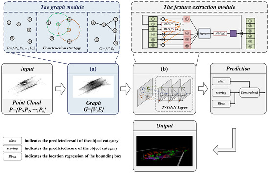
Figure 1. Framework overview.

The graph module utilizes the mapping function to determine the number of grids and points, which obtains the sparse point cloud with retaining enriched information. Then, the vertex and edge features of the graph representation are constructed by searching the neighbors with a fixed radius.

The feature extraction module achieves information transfer by sharing structural features between vertices and edges. In the iteration process, to update the vertices and reduce the offset error, the aggregated feature vectors are computed with the neighbor and edge features. In addition, to avoid repeated grouping and sampling, the edge features of each layer are reused for feature learning.

The prediction module calculates a weighted sum using the location and scale information, which is used to correct the scores of the classification. Then, the bounding box regression prediction is calculated by combining all overlapping bounding boxes of the prediction object.

3.2. The Point Cloud Processing Module

The LiDAR point cloud with a large number of points usually consists of tens of thousands of points. Constructing a graph representation with all points as vertices introduces a huge computational cost, which may lead to an unsatisfactory processing speed in the model. Therefore, we propose to construct the graph with the point cloud after the down-sampling process. It is worth noting that the voxelization here is only used to reduce the density of the point cloud, and it is not used as a representation of the point cloud for feature extraction.

Therefore, point clouds are sparsely processed in several research works. A common method of point cloud down-sampling is structural voxelization. In this method, the point $p_i$ is assigned to the corresponding voxel $v_j$ according to its spatial coordinates. The down-sampling point cloud is achieved by sampling a fixed number of points in each voxel grid, as shown in Equations (1) and (2):

$$F_v\left(p_i\right)=\left\{\begin{array}{cc}\varnothing ,\hfill & p_{j}isdropped\hfill \\ v_j,\hfill & otherwise\hfill \end{array}\right.$$

(1)

$$F_p\left(v_j\right)=\left\{\begin{array}{cc}\varnothing ,\hfill & v_{j}isdropped\hfill \\ \{p_j\mid \forall p_j\in v_j\},\hfill & \forall j\hfill \end{array}\right.$$

(2)

where $F_v\left(p_i\right)$ denotes the mapping of the voxel $v_j$ where each point $p_i$ is located, and $F_p\left(v_j\right)$ denotes the mapping of the set of points in the voxel $v_j$.

In the structure voxelization method, if the number of assigned points in the voxel grid exceeds the default value, the extra points are dropped. Otherwise, the remaining part will be filled to zero. However, the LiDAR point cloud is a non-Euclidean structure, and the distribution in the point cloud is random and disorderly. If the point cloud is processed using structural voxelization, the critical information might be discarded with high density, as well as adding ineffective space and computational cost with sparse density. Therefore, balancing the density of points and detection accuracy in LiDAR point cloud detection has significant investigative importance.

To address the mentioned limitations, we propose a dynamic sparsification method for point cloud processing, as shown in Figure 2.

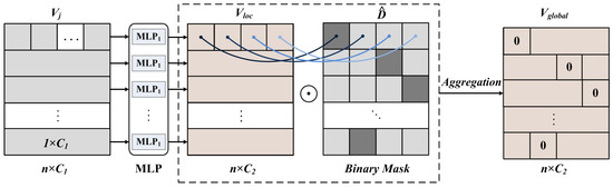
Figure 2. The dynamic sparsification-based point cloud processing. Firstly, we define the expression of the voxel grid as $v_i\in {\mathbb{R}}^{n\times C_1}$. Secondly, to ensure the invariance of the point cloud structure in the spatial domain, the local voxel feature $v_{loc}\in {\mathbb{R}}^{n\times C_2}$ is obtained by mapping the voxel feature $v_i\in {\mathbb{R}}^{n\times C_1}$ using MLP. This feature includes the number of voxel grids and the number of points contained in the grid. Then, according to the number of points contained in the grid sort the voxel grid, the binary mask $\widehat{D}$ is obtained. Finally, the local voxel feature expression $v_{l}oc$ and the binary mask $\widehat{D}$ are aggregated to obtain the global voxel feature $v_{global}\in {\mathbb{R}}^{n\times C_2}$.

We define the point cloud as $P=\{p_0,p_1,\cdots ,p_N\}$. Instead of sampling points to a fixed voxel, we propose to preserve the entire mapping relationship between points and voxels, as shown in Equations (3) and (4):

$$F_v\left(p_i\right)=v_j\in {\mathbb{R}}^{n\times C_1}$$

(3)

$$F_p\left(v_j\right)=\{p_j\mid \forall p_j\in v_j\}\forall j$$

(4)

We analyze the random sampling method for reducing the density of the point cloud, which will not ensure that the point cloud preserves the complete critical information.

Firstly, the constructed voxel feature $v_i\in {\mathbb{R}}^{n\times C_1}$ is mapped to the local voxel feature $v_{loc}$, which contains information about the number of dynamic voxel grids, as shown in Equation (5):

$$v_{loc}=MLP\left(v_j\right)\in {\mathbb{R}}^{n\times C_2}$$

(5)

Secondly, the local voxel feature $v_{loc}\in {\mathbb{R}}^{n\times C_2}$ is aggregated with the binary mask $\widehat{D}\in {\mathbb{R}}^{n\times C_2}$, and the global voxel feature $v_{global}$ is obtained for dynamic sparse point cloud processing, as shown in Equation (6):

$$v_{global}=Agg(v_{loc},\widehat{D})\in {\mathbb{R}}^{n\times C_2}$$

(6)

where Agg() denotes the function that aggregates the available feature information.

Finally, the global voxel feature $v_{global}\in {\mathbb{R}}^{n\times C_2}$ is embedded in $F_p\left(v_i\right)$ as shown in Equations (7) and (8):

$$F_v\left(p_i\right)=v_{global}\in {\mathbb{R}}^{n\times C_2}$$

(7)

$$F_p\left(v_i\right)=\{p_j\mid \forall p_j\in v_{global}\}\forall j$$

(8)

This method eliminates the fixed memory requirements of downsampling operations, and it does not randomly discard points and grids. It can solve the problem of loss of critical information and null operations caused by sparsity and density imbalance in 3D point clouds. The dynamic sparsification method enables dynamic and efficient resource allocation to manage all points and voxels. The ability to generate a deterministic voxel embedding assures more stable detection results with dynamic sparsification.

The point cloud structure only contains information about points, and there is no information about the edges inherently. Therefore, when constructing the graph representation, the definition of edge features needs to be added manually by using the vertex features in the point cloud.

As shown in Figure 3, we are given a point cloud $P=\{p_0,p_1,\cdots ,p_N\}\in {\mathbb{R}}^{n\times C}$, which is used to construct a graph representation $G(V,E)$. We create an edge E by taking $p_i$ as a vertex V and connecting the point to the neighbor within its fixed radius r.

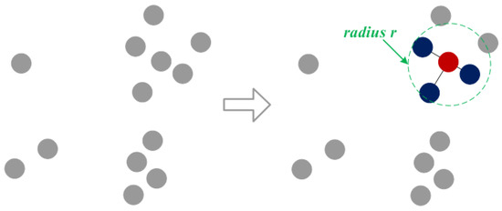
Figure 3. Construction strategy for edge features in the graph. Red indicates the vertex, and blue indicates its neighbors.

We convert the graph representation to a fixed radius nearest neighbor search problem. The runtime complexity $O\left(cN\right)$ problem is efficiently solved by using a list of cells to find pairs of points within a fixed distance, which contains the maximum number of neighbors within the radius, as shown in Equation (9):

$$E=\{(p_i,p_j)\mid \parallel x_j-x_i{\parallel }_2<r\}$$

(9)

3.3. The Feature Extraction Module

We introduce a graph neural network (GNN), which employs standard information transfer to extract features from graph representations. GNNs can maintain the symmetry of the graph information. The vertices are sorted in a different way, which can also guarantee that the prediction results do not change. In the t-th iteration, we set the vertex feature vector to be $S_t$ and the edge feature vector to be $E_t$.

FNRG [27] exploited the consistency of local neighborhood structures to deal with outliers, which is effective for the outlier removal problem. The main reason is that the correspondences preserve local neighborhood structures of feature points. The importance of the neighbor feature structure is demonstrated.

The proposed neighbor feature alignment mechanism is introduced by the example shown in Figure 4. We assume a connection relationship between the centroid $s_3$ and its neighbors ($s_1$,$s_2$ and $s_4$) by denoting s as a vertex and e as an edge. In this case, $e_{(2,3)}$ indicates that there is a connection between the centroid $s_3$ and its neighbor $s_2$. In this example, we can observe the message passing and state updating process of the vertex.

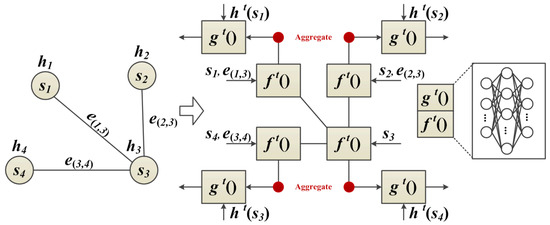
Figure 4. GNN based on neighbor feature alignment mechanism in a single iteration.

The details of our proposed neighbor feature alignment mechanism are introduced as follows.

The classical GNN feature extraction process is shown in Figure 5, where both functions $h^t\left(\right)$ and $f^t\left(\right)$ are Multi-Layer Perceptron (MLP) functions. All vertex features share a multilayer perceptron function, and all edge features share a multilayer perceptron function. In the t+1-th iteration process, the feature vectors of both vertices and edges are updated, and the structure of the graph will not change.

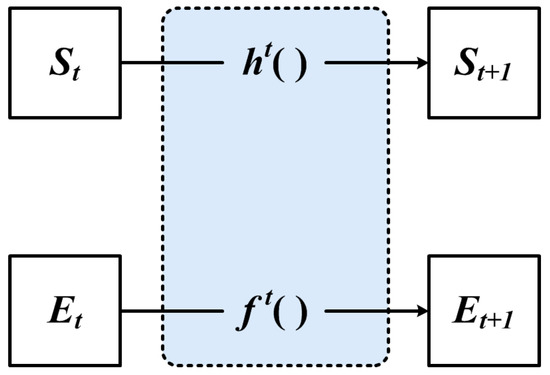
Figure 5. The classical GNN.

However, it can be noticed that there is a problem in the GNN model illustrated in Figure 5, that is, the structural information of the graph is not used in the feature extraction. Although GNN transforms the feature vectors of vertices and edges, there is no information sharing between vertices and edges.

Firstly, we propose to share feature information between vertex and edge features by encoding neighbors, as shown in Figure 6.

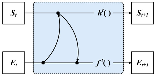
Figure 6. The encoding neighbor method.

In the t+1-th iteration, the updated form of each vertex is as shown in Equation (10):

$$s_i^{t+1}=h^t\left(s_i^t\right)=ML{P}_h^t\left(s_i^t\right)$$

(10)

GNN uses the feature of the vertex to compute the feature of the neighbor, which is used to represent the iterative update process of edge features, as shown in Equation (11):

$$e_i^{t+1}=f^t(x_j-x_i,s_i^t)=ML{P}_f^t\left([x_j-x_i,s_i^t]\right)$$

(11)

However, we use the GNN of Figure 6 for iteration, which can only achieve the encoding of the local neighbor feature, and the original global structure might be lost. Therefore, we propose to use the global structural features aggregated with the local neighbor features in the iteration update process, as shown in Figure 7.

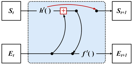
Figure 7. The feature aggregation method.

However, encoding by aggregating local and global information can ensure the information sharing between vertex and edge features, allowing the structural features of the graph to be maximally used. However, the input variables of the function $f^t\left(\right)$ increase when the vertices are shifted, which causes the relative coordinates of the local information to change.

Motivated by the above, we propose a neighbor feature alignment mechanism, as shown in Figure 8.

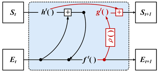
Figure 8. The neighbor feature alignment mechanism.

The GNN based on the neighbor feature alignment mechanism used the structural information from the previous layer of iteration for aligning the relative coordinates, which reduces the sensitivity of local information to the vertex feature offset.

Firstly, we define the coordinate offset representation of the vertex feature as shown in Equation (12):

$$\Delta s_i^t=h^t\left(s_i^t\right)=ML{P}_h^t\left(s_i^t\right)$$

(12)

In the t+1-th iteration process, the edge features are updated by combining with the coordinate offsets of the vertex features, the weighted sum of the local neighbor information, and the global structure information, as shown in Equation (13):

$$e_i^{t+1}=f^t(x_j-x_i+\Delta s_i^t,s_j^t)=ML{P}_f^t([x_j-x_i+\Delta s_i^t,s_j^t])$$

(13)

The state of the vertex features is updated by aggregating the edge features and the global structure information, as shown in Equation (14):

$$s_i^{t+1}=g^t(\rho (\{f^t(x_j-x_i+\Delta s_i^t,s_j^t)\mid (i,j)\in E\}),s_i^t)$$

(14)

where $x_i$ and $x_j$ denote the neighbor features, $\Delta s_i^t$ denotes the coordinate offset of the vertex, and $s_i^t$ denotes the state value of the vertex features from the t-th iteration. The function $f^t\left(\right)$ is used to compute the edge features between vertices, $\rho \left(\right)$ is used to aggregate the edge features of each vertex, $g^t\left(\right)$ updates the state values of the vertices by the aggregated edge features, and $h^t\left(\right)$ computes the offset using the center vertex state values from the previous iteration. It is noted that the offset can be disabled in GNN here by setting $h^t\left(\right)$ to zero. Practically, the functions $f^t\left(\right)$, $g^t\left(\right)$ and $h^t\left(\right)$ are implemented using the MLP, and $\rho \left(\right)$ is chosen to be the mean value.

In summary, the message passing and state updating process of our proposed GNN based on the neighbor feature alignment mechanism is shown in Figure 9.

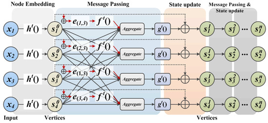
Figure 9. The message passing and state updating process of our method.

3.4. The Prediction Module

In the model prediction stage, we use the output vector of the last layer in the network for prediction. The vertices are represented with feature vectors in the graph, so the network shares a fully connected layer in all vertices, and the classification prediction results are obtained by the Softmax function.

Loss Function

The classification loss is used to calculate the multiclass probability distribution for each vertex. We denote the point cloud as $\{p_{c1},p_{c2},\cdots ,p_{cM}\}$, where M denotes the total number of object classes, including the background classes. In the point cloud-based 3D object detection, then the corresponding object category is assigned to this vertex. If a vertex is located outside of any bounding box, it is classified as the background class. We use the average cross-entropy to calculate the classification loss, as shown in Equation (15):

$${\mathcal{L}}_{cls}=-\frac{1}{N}\sum _{i=1}^N\sum _{j=1}^M[y_{cj}^{i}log(1-p_{cj}^i)+p_{cj}^{i}log(1-y_{cj}^i)]$$

(15)

To calculate the location loss, firstly, the ground truth and the prediction bounding box are parameterized respectively, as shown in Figure 10. We denote the ground truth and prediction bounding box as shown in Equation (16):

$$\begin{array}{c}{c}^{gt}=(x^{gt},y^{gt},z^{gt},l^{gt},w^{gt},h^{gt},{\theta }^{g}t)\hfill \\ c^{pre}=(x^{pre},y^{pre},z^{pre},l^{pre},w^{pre},h^{pre},{\theta }^{pre})\hfill \end{array}$$

(16)

where $(x^{gt},y^{gt},z^{gt})$, and $(x^{pre},y^{pre},z^{pre})$ denotes the center coordinate of ground truth and prediction, respectively. $l^{gt}$,$w^{gt}$,$h^{gt}$ and $l^{pre}$,$w^{pre}$,$h^{pre}$ denotes the length, width, and height of ground truth and prediction, respectively. ${\theta }^{gt}$ and ${\theta }^{pre}$ denote the orientation angle of ground truth and prediction, respectively.

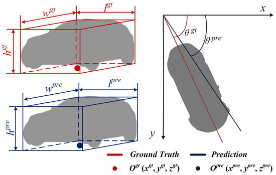
Figure 10. The parameterization of the bounding box.

Then, we transform the original coordinate $c^{gt}$ into the coordinate of GNN vertex ${\Delta }^{gt}$, as shown in Equation (17):

$$\begin{array}{ccc}\Delta x^{gt}=\frac{(x^{gt}-x_v^{gt})}{d^{gt}}\hfill & \Delta y^{gt}=\frac{(y^{gt}-y_v^{gt})}{d^{gt}}\hfill & \Delta z^{gt}=\frac{(z^{gt}-z_v^{gt})}{d^{gt}}\hfill \\ \Delta l^{gt}=log\frac{l^{gt}}{d^{gt}}\hfill & \Delta w^{gt}=log\frac{w^{gt}}{d^{gt}}\hfill & \Delta h^{gt}=log\frac{h^{gt}}{d^{gt}}\hfill \\ \Delta {\theta }^{gt}={\theta }^{gt}\hfill & d^{gt}=\sqrt{{(l^{gt})}^2+{(w^{gt})}^2}\hfill \end{array}$$

(17)

Note that the prediction coordinate uses the same transform strategy.

In general, the Mean Absolute Error (MAE) and the Mean Square Error (MSE) are used to calculate the location loss. However, the model using MAE as the loss function will ignore the outliers, and the model using MSE as the loss function will be biased toward the outliers. Therefore, we propose to calculate the difference between the ground truth and the prediction bounding box with Huber loss[], which is more robust to outliers, as shown in Equation (18):

$${\mathcal{L}}_{\delta }({\Delta }^{pre}-{\Delta }^{gt})=\left\{\begin{array}{cc}\frac{{({\Delta }^{pre}-{\Delta }^{gt})}^2}{2},\hfill & if\mid {\Delta }^{pre}-{\Delta }^{gt}\mid \le \delta \hfill \\ \delta \mid {\Delta }^{pre}-{\Delta }^{gt}\mid -\frac{{\delta }^2}{2},\hfill & otherwise\hfill \end{array}\right.$$

(18)

Then, we calculate the average location loss for all vertices contained in the bounding box, as shown in Equation (19):

$${\mathcal{L}}_{loc}=\frac{1}{N}\sum _{i=1}^N{\mathbb{I}}_{obj}\sum _{\Delta \in {\Delta }_{b_i}}{\mathcal{L}}_{\delta }{\Delta }^{pre}-{\Delta }^{gt}$$

(19)

where the vertex is located within the bounding box, ${\mathbb{I}}_{obj}$ is set to 1, and the loss between the ground truth and the prediction bounding box is calculated. If the vertex is outside any bounding box or it belongs to a category that does not need to be located, ${\mathbb{I}}_{obj}$ is set to 0.

Finally, the loss function in this paper is denoted as Equation (20):

$$\mathcal{L}=\alpha {\mathcal{L}}_{cls}+\beta {\mathcal{L}}_{loc}+\gamma {\mathcal{L}}_{reg}$$

(20)

where $\alpha$, $\beta$, and $\gamma$ denote the trade-off parameters, respectively. ${\mathcal{L}}_{reg}$ denotes $L_2$ regularization, for preventing over-fitting.

4. Experiments and Analysis

The car category has the highest percentage in the KITTI dataset, and we focus on the car category for evaluation. The training set is used for model training, and the validation set is used to evaluate the detection performance of the model.

We will analyze the performance of our method from different perspectives. Firstly, the effectiveness of our method is verified by comparing it with advanced methods in 3D object detection. Secondly, the performance of our method is analyzed by using different iterations and activation functions. Finally, the importance of each module for improving the detection performance is evaluated by a series of ablation studies.

4.1. Dataset and Experimental Details

4.1.1. Datasets

Our method is evaluated quantitatively and qualitatively on the KITTI Object Detection Benchmark [28]. The camera exposure time in the KITTI dataset is controlled by the laser, which triggers the camera shutter when the laser is scanned into the view range of the camera. Therefore, the experiments are conducted only using the view of the camera. For model training and testing, the experiments use the LIDAR point cloud in the lateral range of ±20 m and the distance of 30 m in front of the car.

There is no labeling data in the KITTI test set. Therefore, we have divided the 7481 training samples into training and validation sets, in which the training set contains 3712 samples, and the validation set contains 3769 samples.

4.1.2. Experimental Details

The experimental platform is NVIDIA RTX 3090, CUDA 11.1, Ubuntu 18.04, Python 3.6, and Tensorflow 1.18.1. We use the Tensorflow framework to construct the GNN model. In the training stage, the input sample batch size is selected as 4. The GNN is trained end-to-end, and the trade-off parameters of the loss function are set to $\alpha =0.1$, $\beta =10$, $\gamma$ = 5 × 10${}^{-7}$, respectively. The optimizer uses Adam. The maximum number of input edges for each vertex is limited to 256 in the training process, and all input edges are used in the inference process.

We conduct experiments in three categories (car, pedestrian and cyclist) to verify the performance of our method. Considering the large scale differences between the different categories, for instance, the length of car is about 3–4 m, while the length of pedestrian and rider is about 0.5–1 m and 1.5–2.0 m, respectively. Therefore, we adopt two different experimental setups in the training stage. The specific details are as follows.

For the car category, the initial learning rate of 0.125 and the decay rate of 0.1 are used in the training, and the number of training steps is set to 1,400,000 steps. The length, height, and width of the median in the bounding box are set to 3.88 m, 1.5 m, and 1.63 m, respectively. The graph of the car category is constructed with r = 4 m. The dimensionality of the input feature vectors of functions $f^t\left(\right)$ and $g^t\left(\right)$ is set to (300, 300).

For the pedestrian and cyclist categories, the initial learning rate of 0.32 and the decay rate of 0.25 are used in the training, and the number of training steps is set to 1,000,000 steps. The length, height, and width of the median in the bounding box of the pedestrian are set to 0.9 m, 1.8 m, and 0.7 m, respectively. In addition, the length, height, and width of the median in the bounding box of the cyclist are set to 1.8 m, 1.8 m, and 0.6 m, respectively. The graph is constructed with r = 1.6 m. The dimensionality of the input feature vectors of functions $f^t\left(\right)$ and $g^t\left(\right)$ is set to (256, 256).

4.2. Comparison with Other Advanced Methods

We evaluate three categories of car, pedestrian, and cyclist from the KITTI dataset. The performance between our method and other advanced methods is compared in terms of three detection difficulty cases, Easy, Moderate, and Hard, with 3D object detection performance $A{P}_{3D}$ and 3D location performance $A{P}_{BEV}$ as evaluation metrics.

As shown in Table 1, the results of our methods are compared with the other state-of-the-art methods in the performance of 3D object detection ($A{P}_{3D}$). We classify all methods into voxel-based methods, point-based methods, and point and voxel fusion methods. Some unpublished experimental results are indicated by “-”, and the best experimental results for each are shown in the underlined.

Table 1. The performance of 3D object detection $A{P}_{3D}$ (%).

Method	Modality	Car			Pedestrian			Cyclist
		Easy	Moderate	Hard	Easy	Moderate	Hard	Easy	Moderate	Hard
voxel-based methods
VoxelNet [6]	LiDAR only	77.47	65.11	57.73	39.48	33.69	31.50	61.22	48.36	44.37
PointPillars [14]	LiDAR only	79.05	74.99	68.30	52.08	43.53	41.49	75.78	59.07	52.92
CIA-SSD [13]	LiDAR+Image	89.59	80.20	72.87	-	-	-	-	-	-
Voxel-RCNN [23]	LiDAR only	90.90	81.62	77.06	-	-	-	-	-	-
SE-SSD [29]	LiDAR only	91.49	85.54	77.15	-	-	-	-	-	-
SMS-Net [30]	LiDAR only	89.34	79.04	77.76	-	-	-	-	-	-
MA-MFFC [31]	LiDAR only	92.60	84.98	83.21	-	-	-	-	-	-
point-voxel methods
F-PointNet [32]	LiDAR+Image	81.02	70.39	62.19	51.21	44.89	40.23	71.96	56.77	50.39
PV-RCNN [20]	LiDAR+Image	90.25	81.43	76.82	52.17	43.29	40.29	78.60	63.71	57.65
VIC-Net [33]	LiDAR only	88.25	80.61	75.83	43.82	37.18	35.35	78.29	63.65	57.27
HVPR [34]	LiDAR only	86.38	77.92	73.04	53.47	43.96	40.64	-	-	-
point-based methods
PointRCNN [15]	LiDAR only	86.69	75.64	70.70	47.98	39.37	36.01	74.96	58.82	52.53
3DSSD [16]	LiDAR only	88.36	79.57	74.55	54.64	44.27	40.23	82.48	64.10	56.90
Point-GNN [17]	LiDAR only	88.33	79.47	72.29	51.92	43.77	40.14	78.60	63.48	57.08
IA-SSD [35]	LiDAR only	88.34	80.13	75.04	46.51	39.03	35.60	78.35	61.94	55.70
Ours	LiDAR only	90.63	80.26	74.02	51.43	43.84	40.42	77.36	60.83	57.39

We can observe from Table 1 that, for the car category, our method outperforms all other point-based methods for easy and moderate detection and achieves 90.63% and 80.26%, which outperforms the second-best method +2.27% and +0.13%, respectively. For the pedestrian category, our method outperforms all other point-based methods in difficult detection by 40.42%, which outperforms the second-best method by +0.19%. In addition, the detection performance of moderate, despite not reaching the best, is very close to the state-of-the-art methods. For the cyclist category, our method outperforms all other point-based methods in difficult detection performance by 57.39%, which outperforms the next best method by 0.31%. Despite the pedestrian and cyclist categories, which do not achieve the best results in moderate detection, both of them achieve the best in difficult detection. This indicates that our method can deal well with complex and variable road conditions, and the detection performance is resistant to disturbance.

As shown in Table 2, the results of our method are compared with other advanced methods in terms of 3D location performance ($A{P}_{BEV}$). The best experimental results of each are shown in the underlined.

Table 2. The performance of 3D location performance $A{P}_{BEV}$ (%).

Method	Modality	Car			Pedestrian			Cyclist
		Easy	Moderate	Hard	Easy	Moderate	Hard	Easy	Moderate	Hard
AVOD [36]	LiDAR+Image	88.53	83.79	77.90	58.75	51.05	47.54	68.06	57.48	50.77
F-PointNet [32]	LiDAR+Image	88.70	84.00	75.33	58.09	50.22	47.20	75.38	61.96	54.68
PointPillars [14]	LiDAR only	88.35	86.10	79.83	58.66	50.23	47.19	79.14	62.25	56.00
STD [37]	LiDAR only	89.66	87.76	86.89	60.99	51.39	45.89	81.04	65.32	57.85
Point-GNN [17]	LiDAR only	93.11	89.17	83.90	55.36	47.07	44.61	81.17	67.28	59.67
SMS-Net [30]	LiDAR only	90.34	87.89	87.01	-	-	-	-	-	-
Ours	LiDAR only	96.07	90.79	89.01	58.99	56.01	51.30	81.72	62.53	58.75

We can observe that, for the car category, the 3D location performance achieves 96.9% and 92.18% in easy and moderate, respectively, which outperforms the next best methods +3.51% and +3.01%, respectively. For the pedestrian category, our method achieves 56.01% and 51.30% in moderate and hard, respectively, which outperforms the next best methods +4.62% and +3.49%, respectively. Despite our method not achieving the best result in easy detection, it is very close to the performance of the best result. For the cyclist category, our method achieves 81.72% in easy detection, which outperforms the next best methods by +0.55%. We can find that the cyclist category is not as well detected as the car and pedestrian categories, and one possible reason is the smaller sample of cyclists and the insufficient vertex density that prevents a more accurate prediction, despite the detection performance in the cyclist category not having the best result. However, our method is still able to detect the cyclists well, as shown in Figure 11.

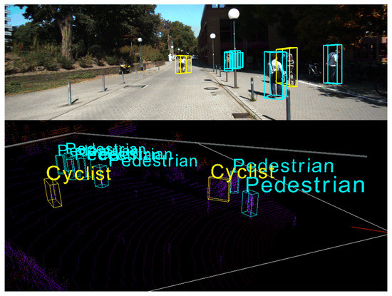
Figure 11. Qualitative results for cyclist and pedestrian categories on the KITTI dataset.

4.3. Ablation Study

4.3.1. The Ablation Study of Activation Function

One of the important properties of a neural network-based model is required to have nonlinearity, which can prevent the model from being a deeply linear classifier. Therefore, firstly, we analyze the effect of different activation functions on model performance. The car category accounts for the highest percentage in the KITTI dataset, and in this section, we focus on the performance evaluation in the car category detection. We use the 3D object detection performance $A{P}_{3D}$ and 3D location performance $A{P}_{BEV}$ as evaluation metrics, and the best results for each are indicated in bold. The EXP.1-EXP.3 denotes the experiments using ReLU, Leaky ReLU, and GELU as the activation layers of the model, respectively.

The experimental results are shown in Table 3. We can observe that the EXP.3 achieves 90.79% and 80.26% detection results on $A{P}_{BEV}$ and $A{P}_{3D}$ with moderate, respectively, which is +5.16% and +2.93% improvement on EXP.1, and +2.42% and +4.22% improvement on EXP.2, respectively. One possible reason is that the GELU activation function introduces the idea of stochastic regularization, which can provide a better representation of the neuronal input. Therefore, we use the GELU activation function in the activation layer.

Table 3. The ablation study for activation function on car category (%).

EXP.	Activation	${\mathit{AP}}_{\mathit{BEV}}$			${\mathit{AP}}_{3\mathit{D}}$
		Easy	Moderate	Hard	Easy	Moderate	Hard
1	ReLU	89.49	85.63	83.02	86.04	74.04	74.68
2	LeakyReLU	94.32	88.37	86.41	89.78	78.33	77.34
3	GELU	96.07	90.79	89.01	90.63	80.26	74.02

4.3.2. The Ablation Study for GNN Iteration

Varying the iteration number of the GNN can refine the state of the vertices in the graph. In this section, we set the iteration number as 0, 1, and 2 to train the model, respectively. T denotes the number of iterations. T = 0 indicates that one iteration is used, and the initial vertex state is used to train the model directly. Moderate detection more closely resembles the real road scenario, so we use the moderate of 3D object detection performance $A{P}_{3D}$ and 3D location performance $A{P}_{BEV}$ as the evaluation metric.

As shown in Table 4, we can observe that the model has the lowest accuracy at $T=0$; this is because the network only contains the state of the initial vertices, and the perceptual field is not extended, which prevents the neighbor information from flowing in the edge features of the graph. In the moderate detection results, T = 1 achieves 90.63% and 80.26% for $A{P}_{BEV}$ and $A{P}_{3D}$, respectively, which represents +2.53% and +0.72% improvement compared to T = 2. We can find that the detection performance has decreased with the increase in model iterations, which is a possible reason that it is more difficult to train the deep model.

Table 4. The ablation study for iteration number on car category (%).

Iteration	${\mathit{AP}}_{\mathit{BEV}}$			${\mathit{AP}}_{3\mathit{D}}$
	Easy	Moderate	Hard	Easy	Moderate	Hard
0	90.08	79.92	75.64	85.10	74.28	70.68
1	96.07	90.79	89.01	90.63	80.26	74.02
2	95.70	88.26	86.76	89.85	79.54	72.59

4.3.3. The Ablation Study for the Proposed Module

In this section, we analyze the impact of the individual modules on the detection performance. The ablation studies are conducted for the point cloud processing method, the neighbors feature alignment method, and the positive correlation constrained method, respectively. The effectiveness of the individual modules is verified on the public benchmark KITTI dataset.

Point cloud processing. The experiments are performed with the same hyper-parameter settings, and we only change the point cloud processing method. In this section, we use the structural voxelization method [6], the dynamic voxelization method [38], and our dynamic sparsification method for the experiments, respectively. The experiments are evaluated on the KITTI dataset of the car category, which uses the inference time and $A{P}_{3D}$ as metrics.

As shown in Table 5, Ours w/SV, Ours w/DV, and Ours denote the point cloud processing with the structural voxelization method, the dynamic voxelization method, and our dynamic sparsification method, respectively. We can observe that Ours achieves 80.26% $A{P}_{3D}$ in moderate detection, which represents a +3.86% improvement over Ours w/DV and a +6.99% improvement over Ours w/SV.

Table 5. The ablation study of point cloud processing method on car category (%).

Methods	${\mathit{AP}}_{3\mathit{D}}$				Time/ms
	Easy	Moderate	Hard	mAP
Ours w/SV	86.78	73.57	70.43	76.93	641
Ours w/DV	89.68	76.68	73.46	79.94	573
Ours	90.63	80.26	74.02	80.85	599

Moderate detection is generally assumed to be the closest to the real driving scenario. The experimental results as shown in Table 5 illustrated that our method is more suitable for the detection in the real driving scenario. In addition, our method achieves a significant improvement in detection accuracy with the inference time close to the other methods.

Neighbors feature alignment mechanism. In this section, we conduct the ablation study on the KITTI dataset car category, which validates the effectiveness of the neighbor feature alignment mechanism. We use the 3D object detection performance $A{P}_{3D}$ as evaluation metrics, and analyze the influence of the neighbor feature alignment method on detection performance. The Ours w/o align denotes the GNN without the neighbor feature alignment mechanism, and the Ours w/align denotes the GNN with the neighbor feature alignment mechanism.

As shown in Table 6, we can observe that the method with neighbors feature alignment (Ours w/align) achieves the best performance in all terms of $A{P}_{3D}$. In the moderate, and hard detection, the results achieve 90.53%, 80.26%, and 74.02%, respectively, which has +4.95%, +1.82%, and +0.13% improvement compared to the method without neighbor feature alignment (Ours w/o align). The experimental result demonstrates the effectiveness of the neighbor feature alignment mechanism.

Table 6. The ablation study of neighbors feature alignment mechanism on car category (%).

Methods	${\mathit{AP}}_{3\mathit{D}}$				Gain
	Easy	Moderate	Hard	mAP
Ours w/o align	85.58	78.98	73.89	78.82	+0.0%
Ours w/align	90.53	80.26	74.02	81.60	↑ 2.78%

4.4. Qualitative Results and Analysis

This section shows the detection results of our method on RGB images and 3D point clouds, respectively. Our method only uses point cloud data for model training, therefore, the predicted 3D bounding box results are projected to RGB images for visualization.

As shown in Figure 12, the visualization results of 3D object detection for the car (green), the pedestrian (blue), and the cyclist (yellow) are visualized (point cloud and RGB images) in the KITTI dataset, and the effectiveness of our method is analyzed by qualitative analysis. In particular, row 1 is the visualization results of RGB images, and row 2 is the visualization results of 3D point cloud. It is demonstrated that our method can address the complex and variable road scenario, which is more resistant to interference and is satisfied with the detection requirements of the real road scenario.

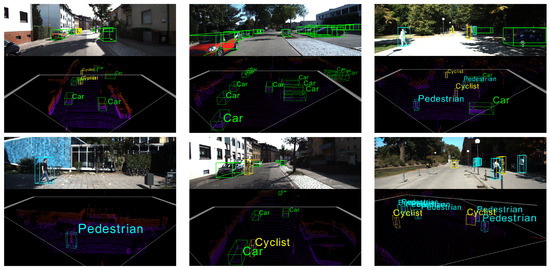
Figure 12. The qualitative results on the KITTI dataset.

5. Conclusions

In this work, we have proposed a graph neural network detector based on neighbor feature alignment mechanism for 3D object detection. This method used 3D point clouds as input with an end-to-end detection framework, which mainly includes point cloud processing, feature extraction, and prediction module. Firstly, we have proposed a dynamic sparsification method to downsample the LiDAR point cloud, which ensures that the critical information of the point cloud is not lost. Secondly, we have proposed a neighbors feature alignment mechanism, which utilizes the structural information of the previous layer to align the relative coordinates, which reduces the sensitivity of neighbors to vertex offset. Finally, the experiments on the public benchmark have demonstrated that our method has been significantly improved.

At present, there is no unified interface API for most 3D object detection datasets. The data formats, coordinate definitions, acquisition methods, and evaluation metrics are very dissimilar between the common datasets. Therefore, our current work is only for the particular use case of KITTI dataset. In our subsequent research work, in the subsequent work, we will try to extend this method to a general 3D object detection framework.

References

- Chen, X.; Kundu, K.; Zhang, Z.; Ma, H.; Fidler, S.; Urtasun, R. Monocular 3D Object Detection for Autonomous Driving. In Proceedings of the 2016 IEEE Conference on Computer Vision and Pattern Recognition, Las Vegas, NV, USA, 27–30 June 2016; pp. 2147–2156. [Google Scholar] [CrossRef]
- Mousavian, A.; Anguelov, D.; Flynn, J.; Kosecka, J. 3D Bounding Box Estimation Using Deep Learning and Geometry. In Proceedings of the 2017 IEEE Conference on Computer Vision and Pattern Recognition, Honolulu, HI, USA, 21–26 July 2017; pp. 5632–5640. [Google Scholar] [CrossRef]
- Song, S.; Xiao, J. Deep Sliding Shapes for Amodal 3D Object Detection in RGB-D Images. In Proceedings of the 2016 IEEE Conference on Computer Vision and Pattern Recognition, Las Vegas, NV, USA, 27–30 June 2016; pp. 808–816. [Google Scholar] [CrossRef]
- Yang, B.; Luo, W.; Urtasun, R. PIXOR: Real-time 3D Object Detection from Point Clouds. In Proceedings of the 2018 IEEE Conference on Computer Vision and Pattern Recognition, Salt Lake City, UT, USA, 18–22 June 2018; pp. 7652–7660. [Google Scholar] [CrossRef]
- Engelcke, M.; Rao, D.; Wang, D.Z.; Tong, C.H.; Posner, I. Vote3Deep: Fast object detection in 3D point clouds using efficient convolutional neural networks. In Proceedings of the 2017 IEEE International Conference on Robotics and Automation, Singapore, 29 May–3 June 2017; pp. 1355–1361. [Google Scholar] [CrossRef]
- Zhou, Y.; Tuzel, O. VoxelNet: End-to-End Learning for Point Cloud Based 3D Object Detection. In Proceedings of the 2018 IEEE/CVF Conference on Computer Vision and Pattern Recognition, Salt Lake City, UT, USA, 18–22 June 2018; pp. 4490–4499. [Google Scholar] [CrossRef]
- Charles, R.Q.; Su, H.; Kaichun, M.; Guibas, L.J. PointNet: Deep Learning on Point Sets for 3D Classification and Segmentation. In Proceedings of the 2017 IEEE Conference on Computer Vision and Pattern Recognition, Honolulu, HI, USA, 21–26 July 2017; pp. 77–85. [Google Scholar] [CrossRef]
- Qi, C.R.; Yi, L.; Su, H.; Guibas, L.J. PointNet++: Deep Hierarchical Feature Learning on Point Sets in a Metric Space; Curran Associates Inc.: Red Hook, NY, USA, 2017. [Google Scholar]
- Scarselli, F.; Gori, M.; Tsoi, A.C.; Hagenbuchner, M.; Monfardini, G. The Graph Neural Network Model. IEEE Trans. Neural Netw. 2009, 20, 61–80. [Google Scholar] [CrossRef] [PubMed]
- Krizhevsky, A.; Sutskever, I.; Hinton, G.E. ImageNet Classification with Deep Convolutional Neural Networks. Commun. ACM 2017, 60, 84–90. [Google Scholar] [CrossRef]
- Zhong, Z.; Xiao, G.; Wang, S.; Wei, L.; Zhang, X. PESA-Net: Permutation-Equivariant Split Attention Network for correspondence learning. Inform. Fus. 2022, 77, 81–89. [Google Scholar] [CrossRef]
- Yan, Y.; Mao, Y.; Li, B. SECOND: Sparsely Embedded Convolutional Detection. Sensors 2018, 18, 3337. [Google Scholar] [CrossRef] [PubMed]
- Wu, Z.; Pan, S.; Chen, F.; Long, G.; Zhang, C.; Yu, P.S. A Comprehensive Survey on Graph Neural Networks. IEEE Trans. Neural Netw. Learn. Syst. 2021, 32, 4–24. [Google Scholar] [CrossRef] [PubMed]
- Lang, A.H.; Vora, S.; Caesar, H.; Zhou, L.; Yang, J.; Beijbom, O. PointPillars: Fast Encoders for Object Detection From Point Clouds. In Proceedings of the 2019 IEEE/CVF Conference on Computer Vision and Pattern Recognition, Long Beach, CA, USA, 15–20 June 2019; pp. 12689–12697. [Google Scholar] [CrossRef]
- Shi, S.; Wang, X.; Li, H. PointRCNN: 3D Object Proposal Generation and Detection From Point Cloud. In Proceedings of the IEEE Conference on Computer Vision and Pattern Recognition (CVPR), Long Beach, CA, USA, 15–20 June 2019. [Google Scholar]
- Yang, Z.; Sun, Y.; Liu, S.; Jia, J. 3DSSD: Point-Based 3D Single Stage Object Detector. In Proceedings of the 2020 IEEE/CVF Conference on Computer Vision and Pattern Recognition (CVPR), Seattle, WA, USA, 13–19 June 2020; pp. 11037–11045. [Google Scholar] [CrossRef]
- Shi, W.; Rajkumar, R. Point-GNN: Graph Neural Network for 3D Object Detection in a Point Cloud. In Proceedings of the 2020 IEEE/CVF Conference on Computer Vision and Pattern Recognition, Seattle, WA, USA, 13–19 June 2020; pp. 1708–1716. [Google Scholar] [CrossRef]
- Feng, M.; Gilani, S.Z.; Wang, Y.; Zhang, L.; Mian, A. Relation Graph Network for 3D Object Detection in Point Clouds; Cornell University: Ithaca, NY, USA, 2019; pp. 92–107. [Google Scholar]
- Liu, Z.; Tang, H.; Lin, Y.; Han, S. Point-Voxel CNN for Efficient 3D Deep Learning; Cornell University: Ithaca, NY, USA, 2019. [Google Scholar]
- Shi, S.; Guo, C.; Jiang, L.; Wang, Z.; Shi, J.; Wang, X.; Li, H. PV-RCNN: Point-Voxel Feature Set Abstraction for 3D Object Detection. In Proceedings of the 2020 IEEE Conference on Computer Vision and Pattern Recognition, Seattle, WA, USA, 14–19 June 2020; pp. 10526–10535. [Google Scholar] [CrossRef]
- He, C.; Zeng, H.; Huang, J.; Hua, X.S.; Zhang, L. Structure Aware Single-Stage 3D Object Detection From Point Cloud. In Proceedings of the 2020 IEEE/CVF Conference on Computer Vision and Pattern Recognition, Seattle, WA, USA, 14–19 June 2020; pp. 11870–11879. [Google Scholar] [CrossRef]
- Li, Z.; Yao, Y.; Zhibin, Q.; Yang, W.; Xie, J. SIENet: Spatial Information Enhancement Network for 3D Object Detection from Point Cloud. arXiv 2021, arXiv:2103.15396. [Google Scholar]
- Deng, J.; Shi, S.; Li, P.; Zhou, W.; Zhang, Y.; Li, H. Voxel R-CNN: Towards High Performance Voxel-based 3D Object Detection. arXiv 2020, arXiv:2012.15712. [Google Scholar] [CrossRef]
- Zheng, L.; Xiao, G.; Shi, Z.; Wang, S.; Ma, J. MSA-Net: Establishing Reliable Correspondences by Multiscale Attention Network. IEEE Trans. Image Process. 2022, 31, 4598–4608. [Google Scholar] [CrossRef] [PubMed]
- Chen, S.; Zheng, L.; Xiao, G.; Zhong, Z.; Ma, J. CSDA-Net: Seeking reliable correspondences by channel-Spatial difference augment network. Pattern Recognit. 2022, 126, 108539. [Google Scholar] [CrossRef]
- Zhong, Z.; Xiao, G.; Zheng, L.; Lu, Y.; Ma, J. T-Net: Effective Permutation-Equivariant Network for Two-View Correspondence Learning. In Proceedings of the 2021 IEEE/CVF International Conference on Computer Vision (ICCV), Montreal, QC, Canada, 10–17 October 2021; pp. 1930–1939. [Google Scholar] [CrossRef]
- Xiao, G.; Luo, H.; Zeng, K.; Wei, L.; Ma, J. Robust Feature Matching for Remote Sensing Image Registration via Guided Hyperplane Fitting. IEEE Trans. Geosci. Remote. Sens. 2022, 60, 1–14. [Google Scholar] [CrossRef]
- Geiger, A.; Lenz, P.; Urtasun, R. Are we ready for Autonomous Driving? The KITTI Vision Benchmark Suite. In Proceedings of the Conference on Computer Vision and Pattern Recognition (CVPR), Washington, DC, USA, 16–21 June 2012. [Google Scholar]
- Zheng, W.; Tang, W.; Jiang, L.; Fu, C.-W. SE-SSD: Self-Ensembling Single-Stage Object Detector From Point Cloud. In Proceedings of the CVPR, Online, 19–25 June 2021; pp. 14494–14503. [Google Scholar]
- Liu, S.; Huang, W.; Cao, Y.; Li, D.; Chen, S. SMS-Net: Sparse multi-scale voxel feature aggregation network for LiDAR-based 3D object detection. Neurocomputing 2022, 501, 555–565. [Google Scholar] [CrossRef]
- Liu, M.; Ma, J.; Zheng, Q.; Liu, Y.; Shi, G. 3D Object Detection Based on Attention and Multi-Scale Feature Fusion. Sensors 2022, 22, 3935. [Google Scholar] [CrossRef] [PubMed]
- Qi, C.R.; Liu, W.; Wu, C.; Su, H.; Guibas, L.J. Frustum PointNets for 3D Object Detection from RGB-D Data. In Proceedings of the IEEE Conference on Computer Vision and Pattern Recognition, Salt Lake City, UT, USA, 18–22 June 2018; pp. 918–927. [Google Scholar] [CrossRef]
- Jiang, T.; Song, N.; Liu, H.; Yin, R.; Gong, Y.; Yao, J. VIC-Net:Voxelization Information Compensation Network for Point Cloud 3D Object Detection. In Proceedings of the 2021 IEEE International Conference on Robotics and Automation, Xi’an, China, 30 May–5 June 2021; pp. 13408–13414. [Google Scholar] [CrossRef]
- Noh, J.; Lee, S.; Ham, B. HVPR: Hybrid Voxel-Point Representation for Single-stage 3D Object Detection. In Proceedings of the 2021 IEEE/CVF Conference on Computer Vision and Pattern Recognition, Nashville, TN, USA, 19–25 June 2021; pp. 14600–14609. [Google Scholar] [CrossRef]
- Zhang, Y.; Hu, Q.; Xu, G.; Ma, Y.; Wan, J.; Guo, Y. Not All Points Are Equal: Learning Highly Efficient Point-Based Detectors For 3d Lidar Point Clouds; Cornell University: Ithaca, NY, USA, 2022; pp. 18953–18962. [Google Scholar]
- Ku, J.; Mozifian, M.; Lee, J.; Harakeh, A.; Waslander, S.L. Joint 3D Proposal Generation and Object Detection from View Aggregation. In Proceedings of the 2018 IEEE/RSJ International Conference on Intelligent Robots and Systems, Madrid, Spain, 1–5 October 2018; pp. 1–8. [Google Scholar] [CrossRef]
- Yang, Z.; Sun, Y.; Liu, S.; Shen, X.; Jia, J. STD: Sparse-to-Dense 3D Object Detector for Point Cloud. In Proceedings of the 2019 IEEE/CVF International Conference on Computer Vision, Seoul, Republic of Korea, 27–28 October 2019; pp. 1951–1960. [Google Scholar] [CrossRef]
- Zhou, Y.; Sun, P.; Zhang, Y.; Anguelov, D.; Gao, J.; Ouyang, T.; Guo, J.; Ngiam, J.; Vasudevan, V. End-to-End Multi-View Fusion for 3D Object Detection in LiDAR Point Clouds. In Proceedings of the Conference on Robot Learning, Auckland, NZ, USA, 14–18 December 2020; pp. 923–932. [Google Scholar]
Disclaimer/Publisher’s Note: The statements, opinions and data contained in all publications are solely those of the individual author(s) and contributor(s) and not of MDPI and/or the editor(s). MDPI and/or the editor(s) disclaim responsibility for any injury to people or property resulting from any ideas, methods, instructions or products referred to in the content. |
© 2023 by the authors. Licensee MDPI, Basel, Switzerland. This article is an open access article distributed under the terms and conditions of the Creative Commons Attribution (CC BY) license (https://creativecommons.org/licenses/by/4.0/).