Advanced Motor Control for Improving the Trajectory Tracking Accuracy of a Low-Cost Mobile Robot

Abstract

Accurate trajectory tracking is a paramount objective when a mobile robot must perform complicated tasks. In high-speed movements, time delays appear when reaching the desired position and orientation, as well as overshoots in the changes of orientation, which prevent the execution of some tasks. One of the aspects that most influences the tracking performance is the control system of the actuators of the robot wheels. It usually implements PID controllers that, in the case of low-cost robots, do not yield a good tracking performance owing to friction nonlinearity, hardware time delay and saturation. We propose to overcome these problems by designing an advanced process control system composed of a PID controller plus a prefilter combined with a Smith predictor, an anti-windup scheme and a Coulomb friction compensator. The contribution of this article is the motor control scheme and the method to tune the parameters of the controllers. It has been implemented in a well-known low-cost small mobile robot and experiments have been carried out that demonstrate the improvement achieved in the performance by using this control system.

1. Introduction

For any technical application, having a deep knowledge of the model of a system leads to highly precise and accurate results. The more information you gather about a system, the better control schemes you can design to achieve your aim. This is even more decisive when we think of robotic systems, where precision, velocity and robustness are extremely important goals. However, the information on commercial parts comes at a cost: accurate models are only provided by expensive, high-end brands, while low (middle)-cost manufacturers generally sell their products with few (if any) details on their characteristic parameters. Moreover, their behaviour is usually far from optimal or even non-linear, degrading the controllers performance for most applications. Hence, when we operate systems that contain low-cost parts, a first identification stage must be carried out to effectively design a control scheme. Then, to cope with system non-linearities during operation, a number of control strategies can be applied simultaneously, so that the overall control scheme achieves good performance.

In this work, we present a robotic system consisting of a mecanum-wheeled mobile robot (MWMR) equipped with a two-dof whisker sensor for haptic applications. One of the pursued applications is object recognition, in which the whisker touches several points of the surface of an object estimating their 3D coordinates. Then, a cloud of points on the surface of the object is formed, which allows its recognition by matching these points with the information contained in a data base of objects. The quicker and more accurate the MWMR moves, the more points can be collected in a given period of time, which allows to improve the recognition task. However, a common MWMR has some low-cost parts whose parameters are unknown, or whose behaviour exhibits severe non-linearities. For instance, friction is one of the most common non-linearities in the DC motors used to actuate MWMRs, which can cause tracking errors at low speeds or stick–slip phenomena during start and stop stages. It has, therefore, been extensively studied in the literature [1,2] and its identification and compensation is key to improving the robot motion control [2], especially at low speeds or in the presence of ground surface changes. This is of paramount importance to our application, as we need to perform manoeuvers between short distances to automatically reposition the whisker for continuing the measurements. Many identification techniques, such as least-squares [3], neural networks [4] or algebraic estimation [5,6], have also been applied to estimate friction or other robot parameters.

During the last two decades, many different strategies have been proposed to improve the position control of mobile robots, such as input-output linearization [7], linear optimal control [8], model predictive control [9,10], sliding-mode control [11] or neural network control [12]. These controllers are designed to cope with the complete robot dynamics [13,14]. However, as they do not use low-cost parts in their setups, most of these works do not consider effects such as motor friction in their dynamic models, and the controllers have to deal with this phenomena implicitly. In [15], a low-cost hardware MWMR is controlled using a variation of sliding mode control for trajectory tracking, but they still neglect motor friction.

In this paper, we take a different approach to the position control problem. We focus on the low-level control of the DC motors actuating the MWMR to improve the precision of the movement, as a preliminary step prior to designing a robot position controller, which will be carried out in future works. Because of the low-cost nature of our platform, we found the following problems for its rapid, precise positioning: insufficient data provided from the DC motors manufacturer; non-linear friction of the motors; saturation of the motor control signal in fast manoeuvers; overshoot in the Point-To-Point (PTP) motion; and hardware-induced delay (HID) in the control loop. We have not found any other previous work in the literature that addresses all these phenomena in the control of DC motors for mobile robots applications, but they are studied separately. For instance, friction non-linearities are dealt with in [16,17]. The work in [16] presents a nonlinear friction observer for viscous and Coulomb frictions that can be used in the feedback control loop. In [17], two nested loops are used for position control of the MWMR using a quantitative feedback control strategy, and the authors focus on the low-level control of the DC motors. They take friction into account in the controller design, but they ignore saturation of the motor control signals or the delay in the communications. On the other hand, control signal saturation for Euler-Lagrange systems is studied in [18] using a leakage-type adaptive sliding-mode controller, which reduces chattering while also tracks the reference signal in presence of saturation.

However, we intend to model and deal with all mentioned drawbacks by combining several Advanced Control Process (ACP) techniques that are common in industry. Specifically, the techniques proposed to cope with the problems we found are, respectively, a step-based thorough system identification [19]; estimation of a feed-forward compensation term for Coulomb friction; an anti wind-up scheme for saturation prevention [20,21]; a prefilter combined with the inner loop to avoid overshoot [17]; and a Smith predictor to compensate the HID [22].

We also identify some other problems that have not been addressed in the control scheme, but have been quantified for the definition of a small error gap in the goal achievement. These are: non-zero backlash in the reduction gears, low precision of the equipped encoders and low material quality of the mecanum wheels that induces, for example, stick–slip phenomena during acceleration/deceleration manoeuvers, degrading movement accuracy.

This article is organized as follows. Section 2 describes the robot prototype. Section 3 characterizes the dynamics of this robot. Section 4 is devoted to develop the control system. Section 5 shows some experimental results and conclusions are given in Section 6.

2. Robot Setup

The robotic platform studied here can be divided in two main systems: the MWMR platform and the robotic whisker sensor. A 3D visualization of the complete robotic platform is displayed in Figure 1a while the real platform is depicted in Figure 1b.

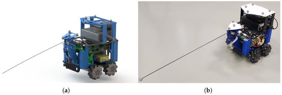
Figure 1. Robotic platform: (a) 3D model; (b) real image.

The main components of the MWMR are the following:

• The chassis, which is equipped with four DC motors with incremental encoders and reduction gears that drive four mecanum wheels (Swedish wheels with rollers at ${45}^{\circ }$). The motors (model GM25-370-24140-75-14.5D10) operate at a voltage control signal within ±9 V, and their reduction gear ratio is 1:75. The encoder resolution is 4 pulses per turn of the motor axle, which corresponds to around 300 pulses per turn of the omni wheel. Hence, the wheel angular position can be measured with an accuracy of $\pm 1.2^{\circ }$.
• A National Instruments Field Programmable Gate Array (FPGA) compactRIO control board, model sbRIO-9631. This card is used to command the motor controllers of the robot (four for the MWMR and two for the whisker), read sensor measurements (encoders and force-torque sensor) and communicate with a host computer via $WiFi$.
• Four servo controller boards Maxon ESCON Module $24/2$. These controllers are mounted on a shield board connected on top of the FPGA and close the inner current loops of the motors, so that the electrical model of each motor can be reduced to a Thevenin equivalent, and the electrical dynamics can be neglected because they are much faster than the mechanical dynamics. They receive the control signals from the FPGA through digital ports and provide the power needed by the motors to operate.
• A router $WiFi$ (model GL.iNet GL-MT300N-V2). This is used to establish wireless communication between the FPGA and an external host computer using a $TCP/IP$ protocol.
• Two 3500 mAh, 3-cell (11.1 V) $LiPo$ batteries connected in series to deliver nominal 22.2 V. They supply the power to the FPGA, the ESCON modules and, using step-down converter from 22 to 5 V, the $WiFi$ router.

The robotic whisker has been defined in previous works [23], and it has been used as a tactile sensor to detect objects surrounding the whisker [24]. Previous whisker setup was static, allowing for a small range of object detection. In order to carry out the already mentioned object recognition application, the sensing range of the whisker has to be increased. This is achieved by mounting it aboard the MWMR which is the object of this study. This poses three main problems: low accuracy and/or precision of the MWMR pose, which significantly degrades sensor measurements; low speed of the MWMR positioning, which reduces the efficiency of the task of collecting points on the surface of the object; and the induction of vibrations to the whisker, which complicates its precise control. Present work deals with the first and second problems, aiming for a precise positioning of the MWMR while using some low-cost parts. Henceforth, the whisker and its servoposition system, that are shown in Figure 1b at the top of the MWMR, will be hereafter omitted.

All work related to data analysis, identification, control design, simulations and data representation have been carried through with Matlab and Simulink R2022a software. Robot hardware is programmed, via the National Instruments Control board with and external computer, using LabView 2019 software.

3. Modeling and Identification

The first obstacle to design the actuator control is the lack of information about the DC motor physical constants: rotor inertia, viscous friction, electromechanical constant and non-linear friction. Therefore, a thorough identification process must first be performed to obtain a mathematical model of the actuators.

3.1. Analytical Model

The dynamic model of each DC motor with 1:n reduction gear ratio is:

$$\mathrm{\Gamma }\left(t\right)=n·K_m·V\left(t\right)=J_m·\ddot{\theta }\left(t\right)+\nu ·\dot{\theta }\left(t\right)+{\mathrm{\Gamma }}_f\left(t\right)+{\mathrm{\Gamma }}_{coup}\left(t\right)$$

(1)

where $\mathrm{\Gamma }\left(t\right)$ is the motor torque, $V\left(t\right)$ the input voltage signal to the motor, $J_m$ and $\nu$ the total inertia and viscous friction of the motor, respectively, $\theta \left(t\right)$ the angle of the motor, ${\mathrm{\Gamma }}_f\left(t\right)$ the non-linear friction term and ${\mathrm{\Gamma }}_{coup}\left(t\right)$ the coupling torque.

The coupling torque ${\mathrm{\Gamma }}_{coup}\left(t\right)$ is the torque that the robot transmits to the wheels and the motors due to its mass and inertia, that this, due to robot dynamics. The moments and forces that robot dynamics induce to the wheels are produced by changes in robot velocity, that is, accelerations. So, neglecting friction terms and considering perfect grip between the wheels and the ground we can approximate the coupling torque (and hence, robot dynamics) to a function of the angular acceleration of the motors for the sake of simplicity:

$${\mathrm{\Gamma }}_{coup}\left(t\right)\approx J_R·\ddot{\theta }\left(t\right)$$

(2)

where $J_R$ is the inertia of the robot that the motors need to overcome. This approximation allow us to simplify (1) and introduce the mass and inertia of the robot in a new inertia term, J:

$$\mathrm{\Gamma }\left(t\right)=n·K_m·V\left(t\right)=J·\ddot{\theta }\left(t\right)+\nu ·\dot{\theta }\left(t\right)+{\mathrm{\Gamma }}_f\left(t\right)$$

(3)

where J is the total inertia: $J=J_m+J_R$.

The voltage $V\left(t\right)$ is the input voltage signal to the motor, which is the control variable of the system. Voltage is the input to a servo amplifier (the servo controller board Maxon ESCON Module) which controls the input current to the motor by means of an internal loop control, as it is represented in Figure 2a, where V is the input voltage, R is the input resistance of the amplifier circuit, $\tilde{k}$ is the gain of the amplifier and $i_m$ is the armature circuit current. The electrical dynamic of this scheme is much faster than the mechanical dynamics of the motor. Thus, electrical dynamics can be rejected and the servo amplifier can be considered as a constant relation $k_e$ between the voltage and the current to the motor: $i_m=V·k_e$ where $k_e$ includes $\tilde{k}$ and R, as it is represented in Figure 2b. The total torque given to the motor ${\mathrm{\Gamma }}_T$ is directly proportional to the armature circuit in the form ${\mathrm{\Gamma }}_T=k_m·i_m$, where $k_m$ is the electromechanical constant of the motor. Thus, the electromechanical constant of the motor servo amplifier system is $K_m=k_e·k_m$.

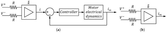
Figure 2. (a) Complete amplifier scheme. (b) Equivalent amplifier scheme.

This model considers simplified robot dynamics as expressed in (2) assuming perfect grip between the wheels and the ground and all the variables are referred to the output of the reduction gear. The transfer function between $V\left(t\right)$ and $\theta \left(t\right)$ can be obtained by removing ${\mathrm{\Gamma }}_f\left(t\right)$ from (3)—because it is considered as a disturbance—and taking Laplace transforms:

$$\widehat{G}\left(s\right)=\frac{\theta \left(s\right)}{V\left(s\right)}=\frac{\frac{n·K_m}{J}}{s^2+\frac{\nu }{J}·s}=\frac{A}{s·(s+B)}$$

(4)

where A and B comprehend the motor parameters which have to be characterized. Then, an identification process is carried out. First, the linear model (4) is identified. Second, taking into account the previous results, a model of the non-linear effects will be identified.

3.2. Identification of the Linear Model

From Equation (4) we can obtain the transfer function between $V\left(t\right)$ and the motor velocity $\dot{\theta }\left(t\right)$:

$$\frac{\dot{\theta }\left(s\right)}{V\left(s\right)}={\widehat{G}}^{{}^{\prime }}\left(s\right)=s·\widehat{G}\left(s\right)=\frac{A}{s+B}$$

(5)

Applying step signals $V\left(t\right)$ of different amplitudes to the motor and measuring the encoder data $\theta \left(t\right)$, the motor parameters of (5) can be determined by using well-known relations of first order systems [25]:

$$B=\frac{3}{t_s},A=P_m·B$$

(6)

where $t_s$ is the settling time (that is, the time needed for the system to enter the ±5% error band of the steady-state value), and $P_m$ is the system gain, which is the relation between the applied voltage and the angular velocity reached in steady-state. Both $t_s$ and $P_m$ are easily obtained from experimental data.

Thus, a series of step signals are generated from 0 to different values between $-6$ V and $+6$ V. This range has been chosen so that it does not become close to the motor limit voltage of 9 V and high and dangerous accelerations of the robot are avoided. The experiments are carried out four times to gather enough data. They were performed simultaneously in all the motors with the robot placed in the ground, allowing it to move along its longitudinal axis. In this way, the parameters of the motor are estimated taking into account the global inertia of the robot. Figure 3 shows some experimental results of the front-left motor.

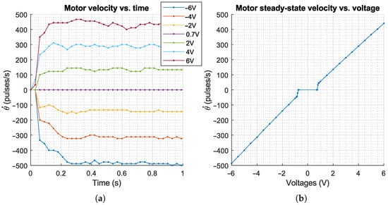
Figure 3. Identification results for front-left motor: (a) motor angular velocity against time for some input voltage steps; (b) steady-state motor angular velocity against voltage supplied for a complete experiment.

Figure 3a represents the motor angular velocities against time. These responses indicate that there is a time delay that must be considered to properly identify the motor parameters. Each of the four experiments will provide four models, one for each motor. Then, sixteen transfer functions will be obtained. Since our objective is to obtain a unique model for all four motors, mean values of the identified parameters A and B will be calculated. The identification of the linear model starts obtaining the values of $P_m$ and $t_s$. Firstly, the parameter $P_m$ is obtained for each experiment and motor from the data collected, as shown in in Figure 3b, which represents the steady-state motor angular velocities—measured in encoder pulses/s—against the supplied voltages. To do that, the steps within the ±1 V region are discarded to focus only in the linear part, where $P_m$ is the slope. There is a slight difference in between the $P_m$ obtained for positive and negative voltage values. This can be blamed on the low quality of the components, because this effect is also observed when running the motors without any load—that means robot dynamics has no influence. Nevertheless, it is such a small error that can be neglected. Secondly, the settling time $t_s$ is obtained from data collected, as shown in Figure 3a. The mentioned time delay is removed in order to obtain the real settling time. Finally, the motor parameters A and B are obtained for every experiment and motor using (6), and the means of the identified sixteen values of A and B yield an average model (4).

The time delay L that appears in the responses of Figure 3a is caused by the speeds of the control board and the ESCON combined with the reduction gears backlash. This parameter is calculated by measuring the time passed by between the instant at which the voltage step is applied and the first instant at which the encoder has a value different from zero. An average value of the time delays obtained in all the experiments is also considered here. Then, the linear dynamics (4) has to be modified to the transfer function

$$G\left(s\right)=\widehat{G}\left(s\right)·e^{-L·s}=\frac{A}{s·(s+B)}·e^{-L·s}$$

(7)

3.3. Identification of Non-Linearities

Once the linear model is obtained, the non-linear effects are modelled and identified. Non-linear friction, saturation of the motors and resolution of the encoder are characterized in this subsection.

3.3.1. Friction Phenomena

Figure 3b shows a discontinuity in between ±1 V approximately, which means that the motor did not move in the experiments in which the step signals where lower than 1 V. This effect is caused by motor internal frictions. This figure shows that the motors have static friction (also known as motor dead-zone) and dynamic friction.

Friction is a well-known phenomena that has been extensively studied [26,27]. Specifically, when using motors to develop high-precision positioning systems, the need to determine friction behaviour and mitigate its effect is of utmost importance. There are several effects related with friction that could appear in DC motors [28]:

• The viscous friction, which is proportional to $\dot{\theta }$ through the viscous friction coefficient $\nu$. It is a linear effect that has already been included in the linear model (7).
• The static friction (stiction) and break-away force. This effect has been observed in Figure 3b, where a discontinuity in $\dot{\theta }$ appears near ±1 V. It occurs when the applied motor torque $\mathrm{\Gamma }\left(t\right)$—expressed in terms of the supplied voltage as expressed in (3)—is lower than the maximum torque generated by the static motor and gearbox internal frictions. This causes the motor to remain stuck without movement. Once $\mathrm{\Gamma }\left(t\right)$ is big enough, the motor starts moving. That is the point where the break-away force is overcome. This phenomenon defines a region called motor dead-zone in which the motor remains stuck when applying torques lower than the break-away torque.
• The Coulomb friction. This friction force appears when the motor is running with non-zero velocity. Its magnitude, which is denoted as the kinetic friction, is constant and its direction is opposite to the motion.
• The Stribeck friction, which is the transition between the stiction and the Coulomb friction. When $\mathrm{\Gamma }\left(t\right)$ overcomes the break-away value, the motor starts running at very low speed and the friction value decreases rapidly. The rapid decrease in the friction value causes an increase in motor velocity, what again causes a friction decrease. This is repeated until the Coulomb friction value is reached. This phenomenon is continuous, depends on the velocity, and occurs in a very short range of velocities.

Dry friction models can be classified in two types [29]: static friction models, which describe the dependence of the friction force on the relative sliding velocity; and dynamic friction models, which take the form of differential equations to not only describe the friction during sliding but also in the stick phase of the frictional elements, i.e., when the measured relative sliding velocity is equal to zero. In practice, the choice between all existing models is strongly influenced by factors such as the available actuators, sensors, and hardware/software control architecture, as well as by constraints on the real-time computational burden [2]. Our MWMR presents some drawbacks related with this factors: lack of information, non-linear behaviour of the actuators, low-precise measures of the sensors and high sample time due to the control board capacity. Therefore, although dynamic models are more precise, we propose a static model because it is much simpler and its parameters are easier to identify. In particular, we chose the Coulomb friction model because it is good enough for the used hardware and the friction coefficients can be identified directly from the experimental data presented in Figure 3b, without further experimentation being required.

Since $\mathrm{\Gamma }\left(t\right)$ is proportional to $V\left(t\right)$, all the friction torques will be hereafter represented by their equivalent voltages. In this way it is avoided having to determine the constant $K_m$, that would have to be used in the implementation of the controller if the model were expressed in function of torques (note that we can obtain parameters A and B from identification, but we cannot obtain $K_m$ neither from identification or from A and B).

The Coulomb friction model ${\mathrm{\Gamma }}_f\left(t\right)$, expressed in terms of its equivalent voltage $V_f\left(t\right)$, is represented in Figure 4a and is modeled through the piecewise function:

$$V_f\left(t\right)=\left\{\begin{array}{cccc}V\left(t\right),\hfill & |\dot{\theta }\left(t\right)|=0\hfill & and\hfill & \left|V\left(t\right)\right|\le V_f^S\hfill \\ V_f^S·sign\left(V\left(t\right)\right),\hfill & |\dot{\theta }\left(t\right)|=0\hfill & and\hfill & \left|V\left(t\right)\right|>V_f^S\hfill \\ V_f^K·sign\left(\dot{\theta }\left(t\right)\right),\hfill & |\dot{\theta }\left(t\right)|\ne 0\hfill \end{array}\right.$$

(8)

where $V_f^S$ is the stiction brake-away equivalent voltage, $V_f^K$ is the kinetic friction equivalent voltage and $V_f^S>V_f^K$. Then, the load torque, i.e., the torque that moves the robot, if expressed in terms of its equivalent voltage, is $V_l\left(t\right)=V\left(t\right)-V_f\left(t\right)$.

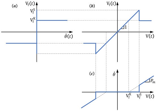
Figure 4. Friction model identification diagrams: (a) Friction torque against motor angular velocity, (b) Friction torque against motor torque, (c) Steady-state motor angular velocity against motor torque.

Figure 4 shows how friction magnitudes $V_f^S$ and $V_f^K$ are identified from the data of Figure 3b. First, these experimental results are represented in Figure 4c as the steady-state velocity against $V\left(t\right)$. Second, in Figure 4b $V_f\left(t\right)$ is represented against $V\left(t\right)$. In addition, friction magnitudes $V_f^S$ and $V_f^K$ are easily identified in the model of the Coulomb friction represented at the left in Figure 4a.

3.3.2. Saturation

There are slight differences between velocities of the motors when running under the same voltage signal. This causes a manoeuvrability problem that impedes the robot to follow a determined trajectory. This problem has been solved in our robot by adjusting a particular saturation voltage for each motor to get all of them to saturate at the same angular velocity, so that the slower motor is the one who determines that maximum speed. Then, a virtual saturation has been established calculating the voltage at which the model identified in (5) runs at the established maximum speed, obtaining the following saturation value $V_{sat}=8.7$ V (saturation voltage of the motors were established by the provider in 9 V).

3.3.3. Encoder Resolution

The incremental encoders only read a change in the motor position when one of the poles is activated. As it was explained before, the encoder has a resolution of 4 pulses each turn of the motor. The relation between the wheel angular position and the measure of the encoder is given by the reduction gear, which was dissembled to find out the exact ratio value. This means that each turn of the wheel corresponds to around 300 pulses, i.e., one encoder pulse is equal to $1.2^{\circ }$. This jump is quite high when controlling the position of the wheels. Thus, to replicate this phenomenon in the model, the signal $\theta \left(t\right)$ will be truncated in the simulations yielding the signal ${\theta }_q\left(t\right)$. This will allow us to assess the impact of this quantization in the control system.

3.4. Identification Results

Identification results are presented in Table 1. Mean values, standard deviations and percentage variances—defined as the maximum difference between the mean value and the most deviated registered data—are provided of both linear and non linear parameters. Note that the maximum variation registered in model parameters is about $14\%$. This data will be used later in the evaluation of the control robustness.

Table 1. Identification results.

Parameters	A	B	L (s)	${\mathit{V}}_{\mathit{f}}^{\mathit{S}}$ (V)	${\mathit{V}}_{\mathit{f}}^{\mathit{K}}$ (V)
Mean value	1631.32	19.97	0.0539	0.85	0.2898
S. deviation	68.66	0.83	0.004	0.00	0.0163
% variance	9.89%	10.81%	14.44%	0%	9.19%

3.5. Complete Model of the System

A block diagram representation of the fully identified motor model is shown in Figure 5. The input $V\left(t\right)$ goes first through a saturation block that limits its maximum absolute value to $V_{sat}$, yielding a voltage signal $V_s\left(t\right)$. After that, the friction block FB$(V,\dot{\theta })$ generates the friction voltage $V_f\left(t\right)$ following the identified model (8). Substracting this value from $V_s\left(t\right)$ gives $V_l\left(t\right)$ which is the voltage equivalent to the torque that moves the linear part of the system. The corresponding nominal transfer function, i.e., transfer function (7) in which the parameters of Table 1 are used, is:

$$G_0\left(s\right)=\frac{\theta \left(s\right)}{V_l\left(s\right)}=\frac{A_0}{s·(s+B_0)}·e^{-L_0·s}=\frac{1631}{s·(s+19.97)}·e^{-0.0539·s}$$

(9)

whose output is $\theta \left(t\right)$. This signal is later differentiated to obtain the velocity $\dot{\theta }\left(t\right)$. Finally, the block ER replicates the encoder resolution yielding a signal ${\theta }_q\left(t\right)$ by truncating $\theta \left(t\right)$.

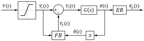
Figure 5. Complete motor model scheme.

4. Control Scheme Design

A control scheme for the motor angle $\theta \left(t\right)$ that combines a PID regulator with a prefilter, a Smith predictor, an antiwindup and a Coulomb friction compensator is proposed. Simulated results will be presented along this section in order to illustrate the problems addressed and how the components that we include in the control system overcome them. Though the analyses will be carried out feeding back the motor angle $\theta \left(t\right)$, the quantized signal ${\theta }_q\left(t\right)$ will be fed back in the simulations.

4.1. PID Regulator with Prefilter

First, a control system is designed for the linear part of the plant in which the time delay has been removed. A loop is closed using a PID regulator, and a prefilter is added to reduce the overshoot of the response. This scheme is shown in Figure 6, where ${\widehat{G}}_0\left(s\right)$ is the linear model (4) with nominal values, ${\theta }^{\ast }\left(t\right)$ is the desired trajectory, $P\left(s\right)$ is the prefilter, ${\theta }_f^{\ast }\left(t\right)$ is the output of the prefilter (and the reference of the closed-loop) and $C\left(s\right)$ is the PID controller:

$$C\left(s\right)=\frac{a_2·s^2+a_1·s+a_0}{s·(s+\mu )}$$

(10)

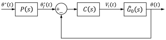
Figure 6. Linear control scheme.

The characteristic equation of the closed-loop system is:

$$\begin{array}{c}\hfill 1+C\left(s\right)·{\widehat{G}}_0\left(s\right)=0\to 1+\frac{a_2·s^2+a_1·s+a_0}{s·(s+\mu )}·\frac{A_0}{s·(s+B_0)}\to \\ \hfill \to s^4+(B_0+\mu )·s^3+(\mu ·B_0+A_0·a_2)·s^2+A_0·a_1·s+A_0·a_0=0\end{array}$$

(11)

Since (11) is a fourth order equation, the closed-loop system has four poles, $p_1$, $p_2$, $p_3$, $p_4$, which are placed in the same position $-p$. Then, the characteristic equation is factorized as

$${(s+p)}^4=0$$

(12)

and the PID parameters are obtained in terms of p equating coefficients of the same order of (11) and (12):

$$\left\{\begin{array}{ccc}\mu \hfill & =\hfill & 4·p-B_0\hfill \\ a_2\hfill & =\hfill & \frac{6·p^2-\mu ·B_0}{A_0}\hfill \\ a_1\hfill & =\hfill & \frac{4·p^3}{A_0}\hfill \\ a_0\hfill & =\hfill & \frac{p^4}{A_0}\hfill \end{array}\right.$$

(13)

The resulting closed-loop transfer function is

$${\widehat{M}}_0\left(s\right)=\frac{\theta \left(s\right)}{{\widehat{\theta }}^{\ast }\left(s\right)}=\frac{C\left(s\right)·{\widehat{G}}_0\left(s\right)}{1+C\left(s\right)·{\widehat{G}}_0\left(s\right)}=\frac{A_0·(a_2·s^2+a_1·s+a_0)}{{(s+p)}^4}$$

(14)

whose zeros are the zeros of the regulator. This produces an undesired overshoot in the step response of ${\widehat{M}}_0\left(s\right)$. For this reason, a prefilter $P\left(s\right)$ is designed. Objectives of the prefilter design are to cancel these zeros to improve the transient response, and to obtain a unit gain response of the closed-loop system to make the response $\theta \left(t\right)$ follow closely the reference ${\theta }^{\ast }\left(t\right)$. Then, the prefilter

$$P\left(s\right)=\frac{p^2·{(s+p)}^2}{A·(a_2·s^2+a_1·s+a_0)}$$

(15)

is used, which cancels two poles of the closed-loop system, reducing the order of the overall system. The resulting transfer function is

$$M_0\left(s\right)=P\left(s\right)·{\widehat{M}}_0\left(s\right)=\frac{p^2}{{(s+p)}^2}$$

(16)

Parameter p is set as big as possible to make the response as fast as possible, but taking into account the limitation of the saturation of the motors. Simulations carried out using a step command ${\theta }^{\ast }\left(t\right)$ of amplitude $\pi$ radians as reference (it is a very demanding command signal) suggest that an adequate value is $p=-10$. This value provides a fast response minimizing the saturation problem. Therefore, the regulator and prefilter parameters are calculated for $p=-10$ using (13) and (15), respectively:

$$C\left(s\right)=\frac{0.1226·s^2+2.452·s+6.13}{s·(s+20.03)}P\left(s\right)=\frac{0.0613·s^2+0.613·s+6.13}{0.1226·s^2+2.452·s+6.13}$$

(17)

4.2. Antiwindup

Since we want to perform very fast trajectories, the control signal may produce motor saturation. In this condition, the control system works in open loop mode because the motor runs at its limit independently of the signal that is being fed back. Furthermore, when the control scheme incorporates an integral action as the one of the designed PID, the error signal keeps being integrated and the integral term of the controller keeps growing. This causes undesired overshoots and increases the time required to reach the desired position. This problem can be alleviated including an antiwindup term in the control system. The control scheme including the PID and the Antiwindup is represented in Figure 7.

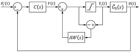
Figure 7. Antiwindup scheme.

Let us express the PID controller (10) in the standard form

$$C\left(s\right)=K+\frac{K}{s{T}_i}+\frac{sK{T}_d}{1+\frac{s{T}_d}{N}}$$

(18)

where the equations of the conversion from (10) are

$$\left\{\begin{array}{ccc}N\hfill & =\hfill & \frac{\mu ·a_2+\frac{a_0}{\mu }-a_1}{a_1-\frac{a_0}{\mu }}\hfill \\ K\hfill & =\hfill & \frac{a_2}{1+N}\hfill \\ T_d\hfill & =\hfill & \frac{N}{\mu }\hfill \\ T_i\hfill & =\hfill & \frac{KN}{a_0·T_d}\hfill \end{array}\right.$$

(19)

Then the antiwindup term $AW\left(s\right)$ of Figure 7 is $K_{AW}/s$, where the antiwindup coefficient is [30] $K_{AW}=1/\sqrt{T_i{T}_d}$. Considering the PID with parameters (17), the theoretical antiwindup coefficient is $K_{AW}=19.9$. However, simulations indicate that the faster response is obtained using $K_{AW}=7$. Figure 8 shows simulated responses to a $2\pi$ radians reference input signal using controller (17) with an antiwindup of $K_{AW}=7$, $K_{AW}=19.9$ and without antiwindup.

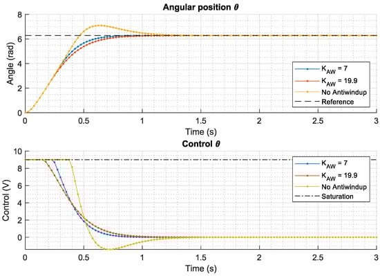
Figure 8. Antiwindup scheme responses.

4.3. Smith Predictor

Even though the identified time delay is not a high value, closed-loop simulations of $G_0\left(s\right)$ with controller (17) and an antiwindup show that it deteriorates the control performance causing overshoot in the motor response. Then, the Smith predictor is developed to improve this response and implemented in the scheme as shown in Figure 9. Figure 10 plots simulated closed-loop step responses with and without a Smith predictor, showing that the overshoot is removed.

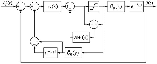
Figure 9. Smith predictor scheme.

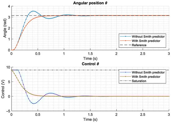
Figure 10. Smith predictor scheme response.

4.4. Friction Compensator

Brake-away and kinetic motor frictions limit the control precision. Precision can be improved by compensating the kinetic friction and maintaining the voltage input outside the motor dead-zone, in such a way that the motor keeps moving until it reaches the desired angle and the error becomes zero. Therefore, a friction compensator FC of the form

$$V_c\left(t\right)=\left\{\begin{array}{cc}{V}_r\left(t\right)+V_f^K·sign\left(V_r\left(t\right)\right),\hfill & |V_r\left(t\right)|+V_f^K>V_f^{min}\hfill \\ V_f^{min}·sign\left(V_r\left(t\right)\right),\hfill & |V_r\left(t\right)|+V_f^K\le V_f^{min}\hfill \end{array}\right.$$

(20)

is proposed where $V_c\left(t\right)$ is the output of the compensator, $V_r\left(t\right)$ is the control signal modified by the antiwindup, and $V_f^{min}=0.9$ V is the minimum voltage provided to the motor, which has been set slightly greater than the stiction brake-away voltage $V_f^S$ to ensure a value outside the motor dead-zone. Simulations of this control system are shown in Figure 11. It is seen that a permanent oscillation is introduced in the steady-state and the motor is unable to drive the motor to the reference.

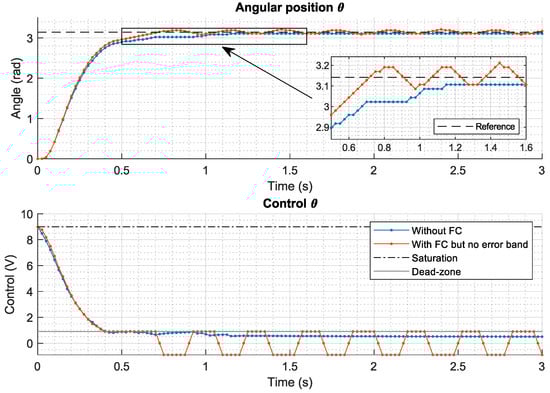
Figure 11. System response with friction compensator (20).

An error band of $\pm e_{min}$ is established to avoid the previous oscillations. $e_{min}$ is determined by the minimum angular displacement that the motor can provide. Since $V_f^{min}$ is the minimum voltage to move the motor, the minimum angular displacement of the motor is obtained when applying $V_f^{min}$ during the controller sampling time, which is 25 ms. Several experiments yielded that a conservative value of this displacement (we want to avoid motor oscillation at all costs) is ±2 pulses, i.e., $e_{min}$ = ±2.4${}^{\circ }$ in each wheel. Note that the quantization error introduced by the encoder is also included in this threshold.

The error band is introduced into the friction compensator (20) as follows:

$$V_c\left(t\right)=\left\{\begin{array}{cc}{V}_r\left(t\right)+V_f^K·sign\left(V_r\left(t\right)\right),\hfill & \left|e\left(t\right)\right|>e_{min}and\left|V_r\left(t\right)\right|+V_f^K>V_f^{min}\hfill \\ V_f^{min}·sign\left(V_r\left(t\right)\right),\hfill & \left|e\left(t\right)\right|>e_{min}and\left|V_r\left(t\right)\right|+V_f^K\le V_f^{min}\hfill \\ 0,\hfill & \left|e\left(t\right)\right|\le e_{min}\hfill \end{array}\right.$$

(21)

where $e\left(t\right)$ is the error between the reference ${\theta }^{\ast }\left(t\right)$ and the encoder measure $\theta \left(t\right)$. Figure 12 represents complete control scheme including friction compensator (21) and Figure 13 shows the simulated closed-loop step response. Note that the motor response is more precise, faster and without overshoot if the friction compensator is used.

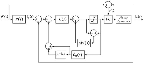
Figure 12. Full control scheme.

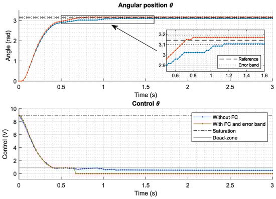
Figure 13. System response with friction compensator and error band (21).

4.5. Stability Analysis

The stability of the closed-loop system is analysed in this subsection because the antiwindup introduces a nonlinearity that can unstabilize the system. In the following analaysis, we will assume that friction effects are completely removed by compensator (21).

The Smith predictor is a well-known scheme which stability has been proven in previous studies [31]. In the case of the nominal plant, it removes the time delay from the closed-loop. Then, the stability analysis of the combination of the PID, the Smith predictor and the antiwindup reduces to the analysis of the PID (18) with the antiwindup $K_{AW}/s$ applied to the process without the time delay, i.e., to ${\widehat{G}}_0\left(s\right)$. This system can be expressed in state-space form [32] as follows:

$$\left\{\begin{array}{ccc}{\displaystyle \frac{dx}{dt}}\hfill & =\hfill & (F-Q·H)·x+(G_r-Q·D_r)·{\theta }^{\ast }-(G-Q·D)·\theta +Q·V_c\hfill \\ U\hfill & =\hfill & H·x+D_r·{\theta }^{\ast }-D·\theta \hfill \\ V_c\hfill & =\hfill & sat\left(U\right)\hfill \end{array}\right.$$

(22)

where the values of the aforementioned vectors and matrices for the proposed controller take the following expressions, which correspond to the observer approach [33]:

$$\begin{array}{cc}F=\left(\begin{array}{cc}0& 0\\ 0& -{\displaystyle \frac{N}{T_d}}\end{array}\right),\hfill & G_r=\left(\begin{array}{c}{\displaystyle \frac{K}{T_i}}\\ {\displaystyle \frac{N}{T_d}}\end{array}\right),G=\left(\begin{array}{c}{\displaystyle \frac{K}{T_i}}\\ {\displaystyle \frac{N}{T_d}}\end{array}\right)\hfill \\ H=\left(\begin{array}{cc}1& -K·N\end{array}\right),\hfill & D_r=K·(1+N)\hfill \\ Q={\left(\begin{array}{cc}{\displaystyle \frac{K_{AW}}{T_i}}& 0\end{array}\right)}^T,\hfill & D=K·(1+N)\hfill \end{array}$$

(23)

where $K_{AW}$ is the antiwindup coefficient and $T_i$, $T_d$, N and K are the controller parameters expressed in the form of (18) that are calculated from the proposed controller (17) as expressed in (19).

As stated in [32], a system with a saturating actuator can always be reduced to the standard Lur’e system configuration with a linear system having a nonlinear feedback. For time invariant monotonic linearities, such as the saturation, sufficient conditions for stability can be obtained from the off-axis circle criterion [34]. Considering that the nonlinear feedback element is saturation, the linear system $G^{\ast }\left(s\right)$ is given by:

$$G^{\ast }\left(s\right)=-\frac{G_c\left(s\right)·{\widehat{G}}_0-W\left(s\right)}{1+W\left(s\right)}$$

(24)

where $G_c\left(s\right)$ and $W\left(s\right)$ are given by the following expressions:

$$\left\{\begin{array}{ccc}W\left(s\right)\hfill & =\hfill & H·{(s·I-F)}^{-1}·Q\hfill \\ G_c\left(s\right)\hfill & =\hfill & H·{(s·I-F)}^{-1}·G+D\hfill \end{array}\right.$$

(25)

being I the identity matrix.

Theorem 1.

If the linear system $G^{\ast }\left(s\right)$ has all its poles in the left half-plane and a nonlinear feedback is closed with a saturation function, the closed loop is absolutely stable provided that a straight line through the origin can be given a nonzero slope, such that $G^{\ast }(j·\omega )+1$ is strictly to the right of the line. $G^{\ast }(j·\omega )+1$ will be strictly positive real (SPR) if it is situated to the right of the imaginary axis.

Proof. 

The proof can be found in ([34], p. 169). □

It is important to note that this theorem is different from Popov’s criterion [35] because $G^{\ast }\left(s\right)$ does not need to be asymptotically stable, i.e., it can present a pole in the origin and because the geometric criterion for the asymptotic stability is that $G^{\ast }\left(i\omega \right)+1$ lies to the right of a line with a slope $q\ne 0$ and is not restricted to the right side of a vertical line, as in Popov’s criterion [36].

The linear system $G^{\ast }\left(s\right)$ for the proposed control scheme is expressed as follows:

$$G^{\ast }\left(s\right)=\frac{\begin{array}{c}\hfill K_{AW}·T_d·s^3+((-(N+1)·A_0·K·T_d·T_i+B_0·K_{AW}·T_d+K_{AW}·N)·s^2+\\ \hfill +(-A_0·K·N·T_i-A_0·K·T_d+B_0·K_{AW}·N)·s-A_0·K·N\end{array}}{\begin{array}{c}\hfill T_d·T_i·s^4+((B_0·T_d+N)·T_i+K_{AW}·T_d)·s^3+\\ \hfill +(B_0·N·T_i+B_0·K_{AW}·T_d+K_{AW}·N)·s^2+B_0·K_{AW}·N·s\end{array}}$$

(26)

where it can be seen that the linear system has all its poles in the left half-plane, and hence, the Theorem can be applied. The stability condition can be expressed as follows:

If there exists a constant $q\ne 0$ such that for all $\omega \ge 0$

$$q·\Re [G^{\ast }(j·\omega )+1]-\Im [G^{\ast }(j·\omega )+1]>0$$

(27)

then the closed-loop system is asymptotically stable.

Numerical evaluation of expression (27) allows us to determine if the combination of the controller and the antiwindup gain leads to a stable closed-loop system. Figure 14 shows the Nyquist diagram of $G^{\ast }\left(s\right)$ (26), and it can be checked that condition (27) is accomplished as the Nyquist plot remains always in the right of the imaginary axis. Therefore, system stability is demonstrated.

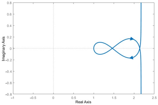
Figure 14. Nyquist diagram of the linear system $G^{\ast }\left(s\right)$.

Robust stability is subsequently checked. 50 simulations have been carried out in which the nominal parameters of Table 1 have been modified randomly in $\pm 20\%$ (it is more demanding than the $\pm 14\%$ variation experimentally assessed). Step responses of all these simulations are represented in Figure 15 compared with the response of the identified nominal mean model. Results prove the convergence to the $\pi$ radians reference in all cases. Moreover, the parameters A and B of the model in Table 1 comprehend robot dynamics (2) as expressed in (4) through the total inertia term J. Then, it is also demonstrated that changes in robot dynamics (variation of A and B) do not affect the control stability of the motors, and therefore, robot dynamics simplification assumed in (2) is considered acceptable for this work.

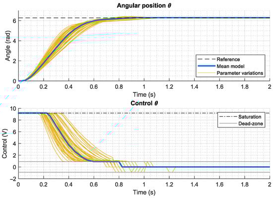
Figure 15. Simulations considering random 20% model parameters variation.

5. Results

Experimental results are presented in this section. The final control scheme represented in Figure 12 is implemented in the National Instruments control board through LabView software and few experiments are carried out. These results present the contribution of the advanced control schemes proposed to cope the non-linearities. The first part resume the obtained results focusing in the main motor behaviour. Then, the robot performance in accurate trajectories tracking and the influence of the advanced control schemes dealing with non-linearities is analysed.

5.1. Motor Control System

Again, a $\pi$ radians step reference is used. The experiments are carried out with the robot on the ground, as it was conducted during the identification part, in order to load the motors with the real torque due to the mass and inertia of the robot.

In the first experiments, responses of the back-right wheel using the PID regulator (17) with and without prefilter are obtained. They are plot in Figure 16. Without prefilter, the transient response presents a big overshoot caused by the zeros of the PID. Once the prefilter defined in (17) is implemented along with the PID, this overshoot is significantly reduced. The remaining overshoot is caused by the saturation of the motor in this demanding reference change, which can be observed in the bottom plot of the figure.

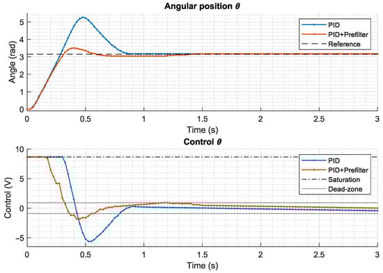
Figure 16. Back-right wheel experimental results with and without prefilter.

Then the antiwindup scheme of Figure 7 is implemented along with the PID and the prefilter. The input reference used here will be twice the previous one, that is: a $2\pi$ radians step reference signal is introduced to the motor control schemes. This reference was used previously during the antiwindup design. It provides better results of the antiwindup behaviour because the motor will saturate for a longer period of time. Thus, Figure 17 compares the response of the back-right wheel without and with the antiwindup, both the angular position and the control voltage. It shows that the antiwindup keeps the motor angle without over passing the reference signal even when introducing higher step reference signals.

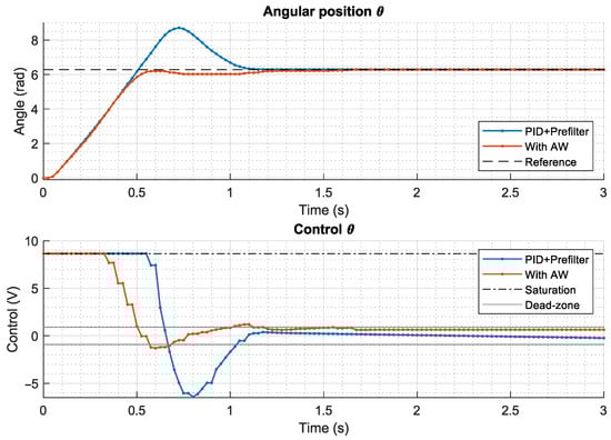
Figure 17. Back-right wheel experimental results with and without Antiwindup.

However, a slight oscillation before reaching the reference is observed in Figure 17. This effect is caused by the time delay and is even more evident when applying the previous $\pi$ radians step reference signal. The response of the control system with the inclusion of the Smith predictor scheme of Figure 9 is represented in Figure 18, both the angular position and the control voltage.

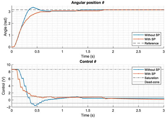
Figure 18. Back-right wheel experimental results with and without Smith predictor.

Now, the motors follow the trajectory as fast as possible without overshoot nor oscillation. However, when the motor is close to reach the reference signal its movement is discontinuous, that is, sometimes it stops and runs intermittently. Moreover, when it definitely stops, it has a noticeable steady-state error. This is the effect of the motor dead-zone (8). As it was explained before, when the control voltage is lower than a threshold the motors stop. This is shown in the control voltage curve: when the voltage gets inside the dead-zone region, motor stops, and control increases again the voltage until motor starts moving again. Introducing the friction compensator (20) in the scheme of Figure 12 yields the results plotted in Figure 19 in which a steady-state error in the range of the resolution of the encoder is obtained but a very small motor angle oscillation appears. Nevertheless, the mean value of the oscillation signal indicates that the steady-state error has been substantially reduced. However, introducing compensator (21) yields the results of Figure 20. This last experimental result shows how this last compensator avoids the small oscillations produced by the previous one while keeping the steady-state error of the motor angle inside the encoder error band.

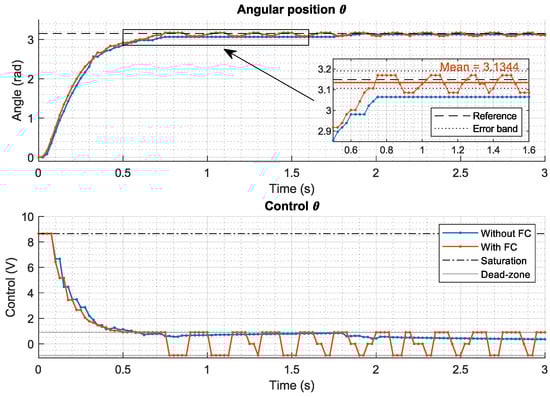
Figure 19. Back-right wheel experimental results with and without friction compensator.

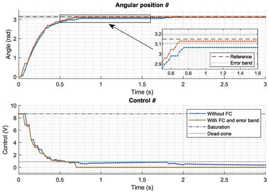
Figure 20. Back-right wheel experimental results with and without friction compensator plus error band.

5.2. Robot Trajectory Tracking

In the pursued application, the robot must perform fast manoeuvers in short distances to automatically reposition the whisker for continuing the haptic measurements. Then, the ability of the MWMR to track fast Cartesian trajectories is assessed. The fastest and most demanding references that can be requested to the robot are the step input signals, which have been used for all along this work. Nevertheless, it is a non desirable reference because it induces very high accelerations to the robot causing unexpected robot behaviors such as wheel slipping and robot wheelies. Thus, a suitable fast input signal is designed with a limited acceleration.

We design a simple Cartesian trajectory in which the robot displaces a determined distance along its longitudinal axis with a limited acceleration and deceleration value. The input reference (in time) consists in three stages: a first stage with constant acceleration in which the robot speeds up until the Cartesian position reaches half of the demanded path, a second stage of constant deceleration (the deceleration of the same magnitude as the acceleration) in which the robot decreases its velocity until it reaches the desired final position with zero velocity, and a steady-state third stage.

Two Cartesian trajectories were tested: a short move of 0.1 m and a long move of 1 m. The maximum acceleration and deceleration value was obtained by experimentation and it was set to 5 m/s². Two sets of three experiments were carried out for each trajectory: the first set performs the manoeuver using our complete control system whereas the second set only uses the PID controller that was designed in Section 4.1 (which is a standard control system for these robots).

Figure 21 shows the time responses of one of the motors in these experiments. When the robot performs the Cartesian 1 m trajectory it is seen that the motor saturates and the PID control is not able to avoid the windup phenomenon, causing an oscillation until it reaches the reference signal. In the case of the Cartesian 0.1 m trajectory, the PID control response shows the expected overshoot due to the identified system delay. Moreover, both manoeuvers show a noticeable steady-state error in the final position angle of the motor compared to the input reference. Nevertheless, it is seen that these problems are avoided by our control system in both experiments, keeping the motors controlled when they saturate, cancelling the overshoot and minimising the steady-state error.

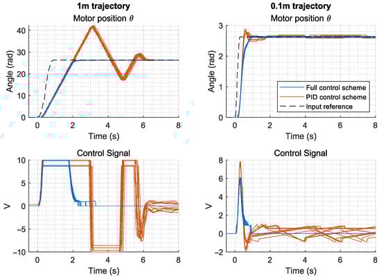
Figure 21. Motor results during robot trajectory tracking.

The PID control weaknesses are directly translated to the evolution (in time) of the robot position, represented in Figure 22. Robot position is measured by an optical camera-based system called Qualisys. As it can be verified in Figure 22, the results improve drastically when using our complete control scheme, approaching the input reference signal closer, earlier and without overshoot if compared with using only the PID controller. Thus, we can conclude that our control also improves robot tracking of Cartesian trajectories.

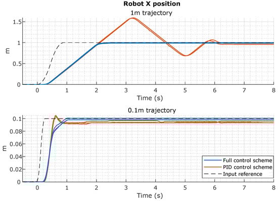
Figure 22. Robot position X results (in time) during robot trajectory tracking.

6. Conclusions

This article has been devoted to improve the positioning and trajectory tracking of a low-cost mecanum-wheeled mobile robot by developing an advanced process control system for the low-level control of the DC motors actuating the MWMR. We have proven that, by using a more sophisticated control system than a PID, a high performance positioning is achieved that will allow us to carry out our haptic application. In fact, by combining a PID with a prefilter, an antiwindup, a Smith predictor and a friction compensator, typical mechanical and hardware problems of low-cost mobile robots such as control overshoots, motor saturation, encoder quantization, hardware induced time delays and nonlinear friction effects are overcome. These components of the control system are well known typical ingredients of the advanced process control systems, that can be easily designed, and their suitability has been proven in industrial applications. Extensive simulations and experiments have proven the efficiency and robustness of the proposed control.

References

- de Wit, C.C.; Lischinsky, P. Adaptive Friction Compensation with Dynamic Friction Model. IFAC Proc. Vol. 1996, 29, 2078–2083. [Google Scholar] [CrossRef]
- Bona, B.; Indri, M. Friction compensation in robotics: An overview. In Proceedings of the 44th IEEE Conference on Decision and Control (CDC-ECC ’05), Seville, Spain, 15 December 2005; pp. 4360–4367. [Google Scholar] [CrossRef]
- Conceição, A.S.; Moreira, P.A.; Costa, P.J. Practical approach of modeling and parameters estimation for omnidirectional mobile robots. IEEE/ASME Trans. Mechatron. 2009, 14, 377–381. [Google Scholar] [CrossRef]
- Rubaai, A.; Kotaru, R. Online Identification and Control of a DC Motor Using Learning Adaptation of Neural Networks. IEEE Trans. Ind. Appl. 2000, 36, 935. [Google Scholar] [CrossRef]
- Ramos, F.; Feliu, V. New online payload identification for flexible robots. Application to adaptive control. J. Sound Vib. 2008, 315, 34–57. [Google Scholar] [CrossRef]
- Mamani, G.; Becedas, J.; Feliu-Batlle, V.; Sira-Ramírez, H. Open-and closed-loop algebraic identification method for adaptive control of DC motors. Int. J. Adapt. Control Signal Process. 2009, 23, 1097–1103. [Google Scholar] [CrossRef]
- Hendzel, Z.; Kolodziej, M. Robust Tracking Control of Omni-Mecanum Wheeled Robot. Adv. Intell. Syst. Comput. 2021, 1390, 219–229. [Google Scholar] [CrossRef]
- Tu, K.Y. A linear optimal tracker designed for omnidirectional vehicle dynamics linearized based on kinematic equations. Robotica 2010, 28, 1033–1043. [Google Scholar] [CrossRef]
- Bouzoualegh, S.; Guechi, E.H.; Kelaiaia, R. Model Predictive Control of a Differential-Drive Mobile Robot. Acta Univ. Sapientiae Electr. Mech. Eng. 2018, 10, 20–41. [Google Scholar] [CrossRef]
- Moreno-Caireta, I.; Celaya, E.; Ros, L. Model Predictive Control for a Mecanum-wheeled Robot Navigating among Obstacles. IFAC-PapersOnLine 2021, 54, 119–125. [Google Scholar] [CrossRef]
- Ovalle, L.; Ríos, H.; Llama, M.; Santibáñez, V.; Dzul, A. Omnidirectional mobile robot robust tracking: Sliding-mode output-based control approaches. Control Eng. Pract. 2019, 85, 50–58. [Google Scholar] [CrossRef]
- Szeremeta, M.; Szuster, M. Neural Tracking Control of a Four-Wheeled Mobile Robot with Mecanum Wheels. Appl. Sci. 2022, 12, 5322. [Google Scholar] [CrossRef]
- Dhaouadi, R.; Hatab, A.A. Dynamic Modelling of Differential-Drive Mobile Robots using Lagrange and Newton-Euler Methodologies: A Unified Framework. Adv. Robot. Autom. 2013, 2, 1–7. [Google Scholar] [CrossRef]
- Hendzel, Z.; Rykała, Ł. Modelling of dynamics of a wheeled mobile robot with mecanum wheels with the use of lagrange equations of the second kind. Int. J. Appl. Mech. Eng. 2017, 22, 81–99. [Google Scholar] [CrossRef]
- Alakshendra, V.; Chiddarwar, S. Adaptive robust control of Mecanum-wheeled mobile robot with uncertainties. Nonlinear Dyn. 2017, 87, 2147–2169. [Google Scholar] [CrossRef]
- Ruderman, M.; Iwasaki, M. Observer of nonlinear friction dynamics for motion control. IEEE Trans. Ind. Electron. 2015, 62, 5941–5949. [Google Scholar] [CrossRef]
- Comasolivas, R.; Quevedo, J.; Escobet, T.; Escobet, A.; Romera, J. Modeling and Robust Low Level Control of an Omnidirectional Mobile Robot. J. Dyn. Syst. Meas. Control Trans. ASME 2017, 139, 041011. [Google Scholar] [CrossRef]
- Shao, K.; Tang, R.; Xu, F.; Wang, X.; Zheng, J. Adaptive sliding mode control for uncertain Euler–Lagrange systems with input saturation. J. Frankl. Inst. 2021, 358, 8356–8376. [Google Scholar] [CrossRef]
- Wu, W. DC motor parameter identification using speed step responses. Model. Simul. Eng. 2012, 2012, 189757. [Google Scholar] [CrossRef]
- Rodriguez, A.S.M.; Hosseini, M.; Paik, J. Hybrid Control Strategy for Force and Precise End Effector Positioning of a Twisted String Actuator. IEEE/ASME Trans. Mechatron. 2021, 26, 2791–2802. [Google Scholar] [CrossRef]
- Gruzman, M.; Weber, H.I.; Menegaldo, L.L. Time Domain Simulation of a Target Tracking System with Backlash Compensation. Math. Probl. Eng. 2010, 2010, 973482. [Google Scholar] [CrossRef]
- Santos, J.; Conceição, A.G.; Santos, T.L. Trajectory tracking of Omni-directional Mobile Robots via Predictive Control plus a Filtered Smith Predictor. IFAC-PapersOnLine 2017, 50, 10250–10255. [Google Scholar] [CrossRef]
- Castillo-Berrio, C.F.; Feliu-Batlle, V. Vibration-free position control for a two degrees of freedom flexible-beam sensor. Mechatronics 2015, 27, 1–12. [Google Scholar] [CrossRef]
- Mérida-Calvo, L.; Feliu-Talegón, D.; Feliu-Batlle, V. Improving the Detection of the Contact Point in Active Sensing Antennae by Processing Combined Static and Dynamic Information. Sensors 2021, 21, 1808. [Google Scholar] [CrossRef] [PubMed]
- Ogata, K. Modern Control Engineering; Prentice Hall: Upper Saddle River, NJ, USA, 2010; Volume 5. [Google Scholar]
- Olsson, H.; Åström, K.J.; Canudas De Wit, C.; Gäfvert, M.; Lischinsky, P. Friction Models and Friction Compensation. Eur. J. Control 1998, 4, 176–195. [Google Scholar] [CrossRef]
- Pennestrì, E.; Rossi, V.; Salvini, P.; Valentini, P.P. Review and comparison of dry friction force models. Nonlinear Dyn. 2016, 83, 1785–1801. [Google Scholar] [CrossRef]
- Virgala, I.; Frankovský, P.; Kenderová, M. Friction Effect Analysis of a DC Motor. Am. J. Mech. Eng. 2013, 1, 1–5. [Google Scholar] [CrossRef]
- Olejnik, P.; Awrejcewicz, J.; Fečkan, M. Modeling, Analysis and Control of Dynamical Systems with Friction and Impacts; World Scientific Publishing Co.: Singapore, 2017; pp. 1–262. [Google Scholar] [CrossRef]
- Åström, T.K. PID Controllers: Theory, Design, and Tunning, 2nd ed.; Instrument Society of America (ISA): Research Triangle Park, NC, USA, 1995. [Google Scholar]
- Bahill, A.T. Simple Adaptive Smith-Predictor for Controlling Time-Delay Systems. IEEE Control Syst. Mag. 1983, 3, 16–22. [Google Scholar] [CrossRef]
- Rundqwist, L. Anti-reset Windup for PID Controllers. IFAC Proc. Vol. 1990, 23, 453–458. [Google Scholar] [CrossRef]
- Åström, K.J.; Wittenmark, B. Computer-Controlled Systems: Theory and Design; Courier Corporation: Englewood Cliffs, NJ, USA, 2013. [Google Scholar]
- Narendra, K.S.; Taylor, J.H. Frequency Domain Criteria for Absolute Stability; Academic Press, Inc.: New York, NY, USA, 1973. [Google Scholar]
- Popov, V. Absolute stability of nonlinear systems of automatic control. Autom. Remote Control 1962, 22, 857–875. [Google Scholar]
- Cho, Y.S.; Narendra, K.S. An Off-Axis Circle Criterion for the Stability of Feedback Systems with a Monotonic Nonlinearity. IEEE Trans. Autom. Control 1968, 13, 413–416. [Google Scholar] [CrossRef]
Disclaimer/Publisher’s Note: The statements, opinions and data contained in all publications are solely those of the individual author(s) and contributor(s) and not of MDPI and/or the editor(s). MDPI and/or the editor(s) disclaim responsibility for any injury to people or property resulting from any ideas, methods, instructions or products referred to in the content. |
© 2022 by the authors. Licensee MDPI, Basel, Switzerland. This article is an open access article distributed under the terms and conditions of the Creative Commons Attribution (CC BY) license (https://creativecommons.org/licenses/by/4.0/).