
A Deep-LSTM-Based Fault Detection Method for Railway Vehicle Suspensions


Abstract
1. Introduction
2. Fundamentals
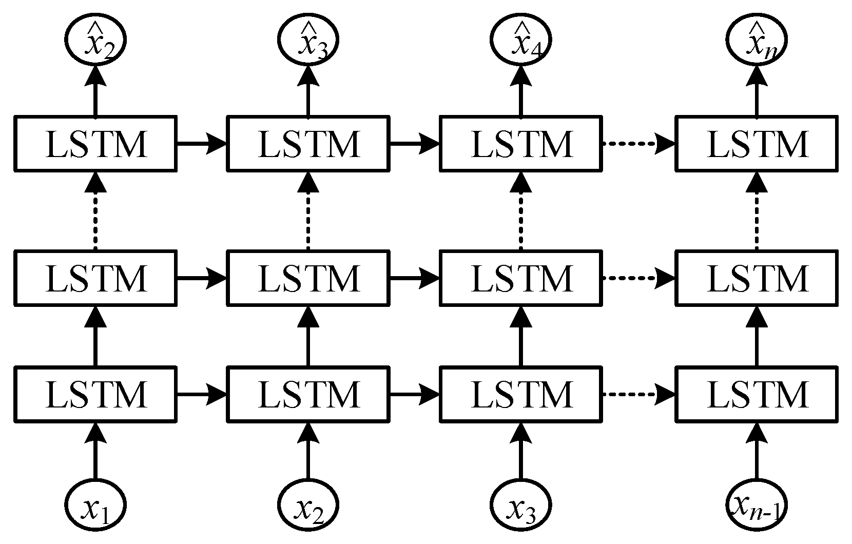
2.1. Deep LSTM
2.2. Architecture Selection and Training Hyperparameter Determination
- (1)
- Configure search candidate sets for each hyperparameter. For instance, the set for Nh1 is = [10:10:100 150:50:1200], where 10:10:100 denotes a sequence from 10 to 100 with an increment of 10.
- (2)
- Use training data to train deep LSTM given specific hyper-parameter values, and then obtain the validation error.
- (3)
- Repeat step (2) until all possible combinations of hyperparameters are evaluated.
- (4)
- Find the combination of hyperparameters that gives the minimal validation error.
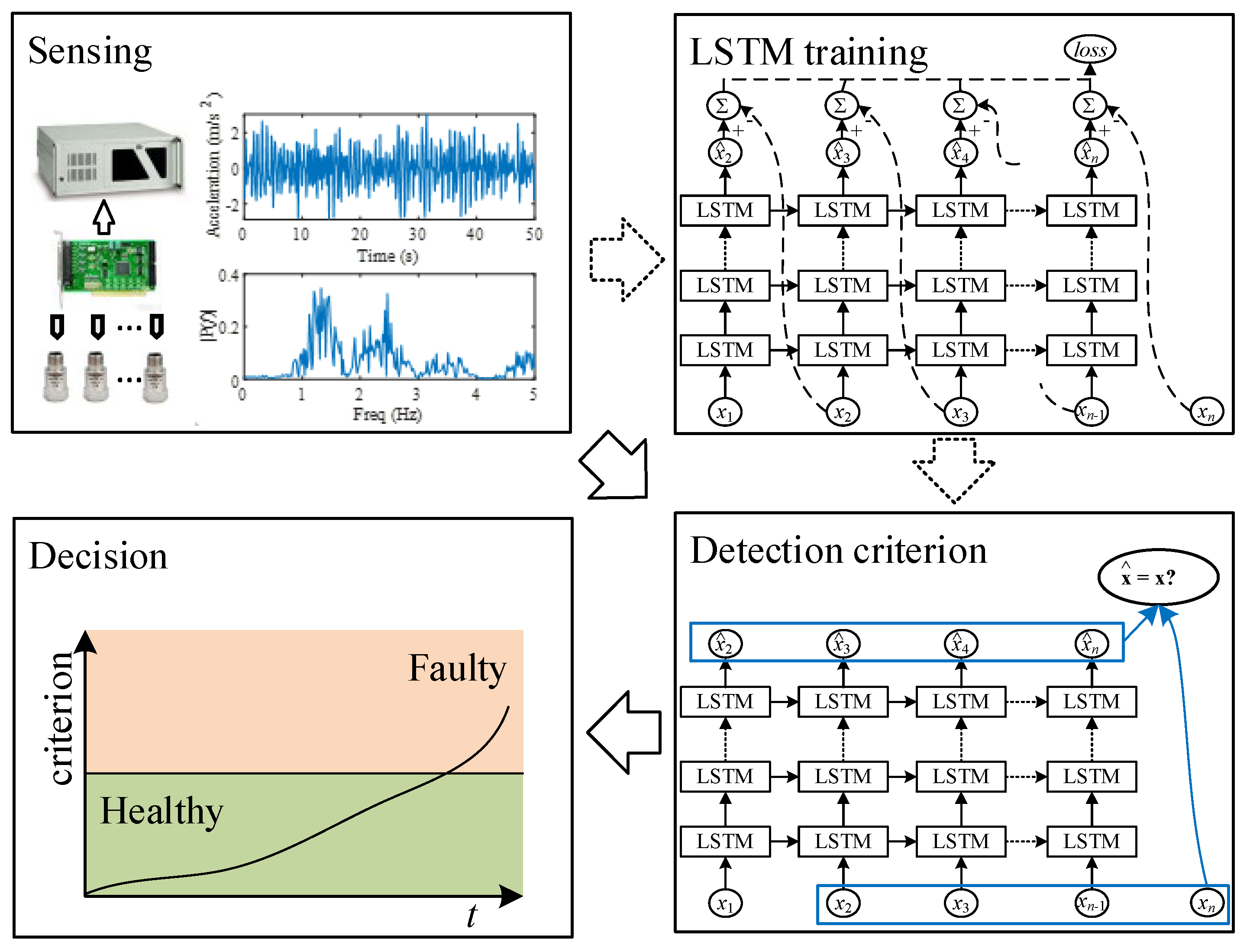
3. Deep-LSTM-Based Fault Detection Method
4. Detection of Railway Vehicle Suspension Faults
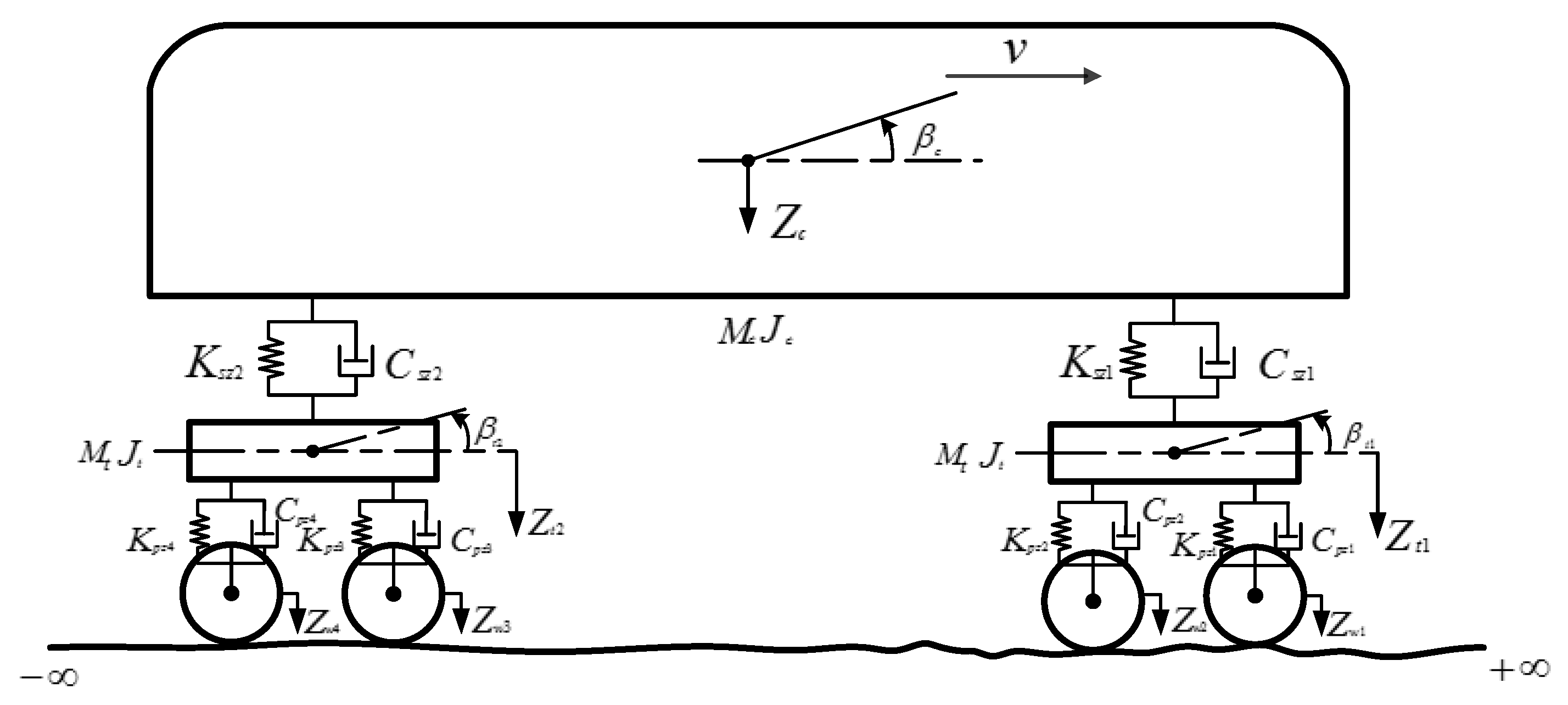
4.1. Railway Vehicle Dynamics Model
- The car body is symmetric and rigid.
- The bogies have a symmetric and rigid body.
- The wheel is modeled as a massless point that follows the rail surface.
- The damping and stiffness are fixed constants.
4.2. Simuluation Configuration
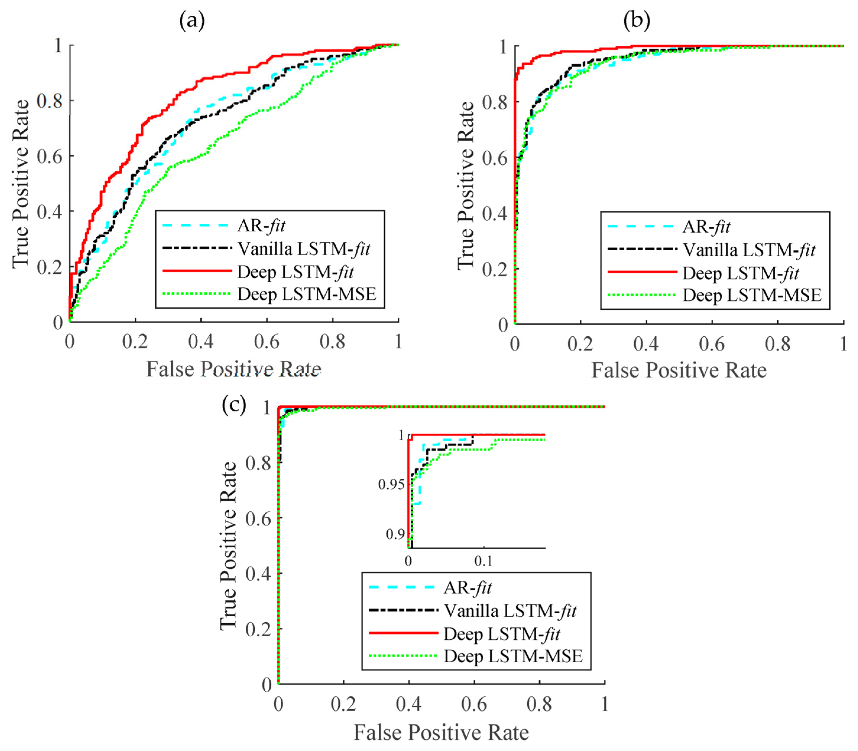
4.3. Performance of the Deep-LSTM–Based Fault Detection Method
5. Discussion
6. Conclusions
Author Contributions
Funding
Data Availability Statement
Acknowledgments
Conflicts of Interest
References
- Pascal, V.; Toufik, A.; Manuel, A.; Florent, D.; Frédéric, K. Improvement indicators for Total Productive Maintenance policy. Control. Eng. Pract. 2018, 82, 86–96. [Google Scholar] [CrossRef]
- Pimentel, M.A.; Clifton, D.A.; Clifton, L.; Tarassenko, L. A review of novelty detection. Signal Process. 2014, 99, 215–249. [Google Scholar] [CrossRef]
- Clifton, L.; Clifton, D.A.; Watkinson, P.J.; Tarassenko, L. Identification of patient deterioration in vital-sign data using one-class support vector machines. In Proceedings of the 2011 Federated Conference on Computer Science and Information Systems (FedCSIS), Szczecin, Poland, 18–21 September 2011; pp. 125–131. [Google Scholar]
- Diehl, C.; Hampshire, J. Real-time object classification and novelty detection for collaborative video surveillance. In Proceedings of the 2002 International Joint Conference on Neural Networks (IJCNN), Honolulu, HI, USA, 12–17 May 2002. [Google Scholar]
- Schmidt, S.; Heyns, P.S.; Gryllias, K.C. A discrepancy analysis methodology for rolling element bearing diagnostics under variable speed conditions. Mech. Syst. Signal Process. 2018, 116, 40–61. [Google Scholar] [CrossRef]
- Li, Y.; Yang, Y.; Wang, X.; Liu, B.; Liang, X. Early fault diagnosis of rolling bearings based on hierarchical symbol dynamic entropy and binary tree support vector machine. J. Sound Vib. 2018, 428, 72–86. [Google Scholar] [CrossRef]
- Liu, Z.; Kang, J.; Zhao, X.; Zuo, M.J.; Qin, Y.; Jia, L. Modeling of the safe region based on support vector data description for health assessment of wheelset bearings. Appl. Math. Model. 2019, 73, 19–39. [Google Scholar] [CrossRef]
- Kim, D.; Kang, P.; Cho, S.; Lee, H.-J.; Doh, S. Machine learning-based novelty detection for faulty wafer detection in semiconductor manufacturing. Expert Syst. Appl. 2012, 39, 4075–4083. [Google Scholar] [CrossRef]
- Sakurada, M.; Yairi, T. Anomaly Detection Using Autoencoders with Nonlinear Dimensionality Reduction. In Proceedings of the MLSDA 2014 2nd Workshop on Machine Learning for Sensory Data Analysis—MLSDA’14, Gold Coast, Australia, 2 December 2014; Association for Computing Machinery (ACM): New York, NY, USA; p. 4. [Google Scholar]
- Wang, W.; Wong, A.K. Autoregressive Model-Based Gear Fault Diagnosis. J. Vib. Acoust. 2002, 124, 172–179. [Google Scholar] [CrossRef]
- Assaad, B.; Eltabach, M.; Antoni, J. Vibration based condition monitoring of a multistage epicyclic gearbox in lifting cranes. Mech. Syst. Signal Process. 2013, 42, 351–367. [Google Scholar] [CrossRef]
- Yip, L. Analysis and Modeling of Planetary Gearbox Vibration Data for Early Fault Detection. Master’s Thesis, University of Toronto (Canada), Toronto, ON, Canada, 2011. Available online: https://search.proquest.com/pqdtglobal/docview/926973307/abstract/DD1FB488429849ACPQ/1 (accessed on 15 December 2017).
- Chen, Y.; Liang, X.; Zuo, M.J. Sparse time series modeling of the baseline vibration from a gearbox under time-varying speed condition. Mech. Syst. Signal Process. 2019, 134, 106342. [Google Scholar] [CrossRef]
- Kim, Y.; Kim, J.; Kim, Y.H.; Chong, J.; Park, H.S. System identification of smart buildings under ambient excitations. Measurement 2016, 87, 294–302. [Google Scholar] [CrossRef]
- Ma, J.; Xu, F.; Huang, K.; Huang, R. GNAR-GARCH model and its application in feature extraction for rolling bearing fault diagnosis. Mech. Syst. Signal Process. 2017, 93, 175–203. [Google Scholar] [CrossRef]
- Chen, R.; Tsay, R.S. Functional-Coefficient Autoregressive Models. J. Am. Stat. Assoc. 1993, 88, 298–308. [Google Scholar] [CrossRef]
- Cai, Z.; Fan, J.; Yao, Q. Functional-Coefficient Regression Models for Nonlinear Time Series. J. Am. Stat. Assoc. 2000, 95, 941–956. [Google Scholar] [CrossRef]
- Fan, J.; Yao, Q.; Cai, Z. Adaptive Varying-Coefficient Linear Models. J. R. Stat. Soc. Ser. B Stat. Methodol. 2003, 65, 57–80. [Google Scholar] [CrossRef]
- Ma, S.; Song, P.X.-K. Varying Index Coefficient Models. J. Am. Stat. Assoc. 2015, 110, 341–356. [Google Scholar] [CrossRef]
- Gan, M.; Peng, H.; Peng, X.; Chen, X.; Inoussa, G. A locally linear RBF network-based state-dependent AR model for nonlinear time series modeling. Inf. Sci. 2010, 180, 4370–4383. [Google Scholar] [CrossRef]
- Gan, M.; Chen, C.L.P.; Li, H.-X.; Chen, L. Gradient Radial Basis Function Based Varying-Coefficient Autoregressive Model for Nonlinear and Nonstationary Time Series. IEEE Signal Process. Lett. 2014, 22, 809–812. [Google Scholar] [CrossRef]
- Yu, Y.; Si, X.; Hu, C.; Zhang, J. A Review of Recurrent Neural Networks: LSTM Cells and Network Architectures. Neural Comput. 2019, 31, 1235–1270. [Google Scholar] [CrossRef] [PubMed]
- Staudemeyer, R.C.; Morris, E.R. Understanding LSTM—A tutorial into Long Short-Term Memory Recurrent Neural Networks. arXiv 2020, arXiv:1909.09586. Available online: http://arxiv.org/abs/1909.09586 (accessed on 15 December 2020).
- Marchi, E.; Vesperini, F.; Squartini, S.; Schuller, B. Deep Recurrent Neural Network-Based Autoencoders for Acoustic Novelty Detection. Comput. Intell. Neurosci. 2017, 2017, e4694860. [Google Scholar] [CrossRef]
- Liu, H.; Zhou, J.; Zheng, Y.; Jiang, W.; Zhang, Y. Fault diagnosis of rolling bearings with recurrent neural network-based autoencoders. ISA Trans. 2018, 77, 167–178. [Google Scholar] [CrossRef]
- Hochreiter, S.; Schmidhuber, J. Long short-term memory. Neural Comput. 1997, 9, 1735–1780. [Google Scholar] [CrossRef]
- Siami-Namini, S.; Tavakoli, N.; Namin, A.S. A Comparison of ARIMA and LSTM in Forecasting Time Series. In Proceedings of the 2018 17th IEEE International Conference on Machine Learning and Applications (ICMLA), Orlando, FL, USA, 17–20 December 2018; pp. 1394–1401. [Google Scholar]
- Ayvaz, E.; Kaplan, K.; Kuncan, M. An Integrated LSTM Neural Networks Approach to Sustainable Balanced Scorecard-Based Early Warning System. IEEE Access 2020, 8, 37958–37966. [Google Scholar] [CrossRef]
- Mao, W.; He, J.; Tang, J.; Li, Y. Predicting remaining useful life of rolling bearings based on deep feature representation and long short-term memory neural network. Adv. Mech. Eng. 2018, 10, 168781401881718. [Google Scholar] [CrossRef]
- Yu, W.; Kim, I.Y.; Mechefske, C. Remaining useful life estimation using a bidirectional recurrent neural network based autoencoder scheme. Mech. Syst. Signal Process. 2019, 129, 764–780. [Google Scholar] [CrossRef]
- Greff, K.; Srivastava, R.K.; Koutník, J.; Steunebrink, B.R.; Schmidhuber, J. LSTM: A Search Space Odyssey. IEEE Trans. Neural Netw. Learn. Syst. 2017, 28, 2222–2232. [Google Scholar] [CrossRef] [PubMed]
- Reimers, N.; Gurevych, I. Optimal Hyperparameters for Deep LSTM-Networks for Sequence Labeling Tasks. arXiv 2021, arXiv:1707.06799. Available online: http://arxiv.org/abs/1707.06799 (accessed on 6 January 2021).
- Cho, K.; Van Merrienboer, B.; Bahdanau, D.; Bengio, Y. On the properties of neural machine translation: Encoder-decoder approaches. arXiv 2014, arXiv:1409.1259. [Google Scholar] [CrossRef]
- Jozefowicz, R.; Zaremba, W.; Sutskever, I. An Empirical Exploration of Recurrent Network Architectures. In Proceedings of the 32nd International Conference on Machine Learning, Lille, France, 6–11 July 2015; pp. 2342–2350. [Google Scholar]
- Yokouchi, T.; Kondo, M. LSTM-based Anomaly Detection for Railway Vehicle Air-conditioning Unit using Monitoring Data. In Proceedings of the IECON 2021—47th Annual Conference of the IEEE Industrial Electronics Society, Toronto, ON, Canada, 13–16 October 2021; pp. 1–6. [Google Scholar]
- Rustam, F.; Ishaq, A.; Alam Hashmi, M.S.; Siddiqui, H.U.R.; López, L.A.D.; Galán, J.C.; Ashraf, I. Railway Track Fault Detection Using Selective MFCC Features from Acoustic Data. Sensors 2023, 23, 7018. [Google Scholar] [CrossRef]
- Eunus, S.I.; Hossain, S.; Ridwan, A.E.M.; Adnan, A. ECARRNet: An Efficient LSTM Based Ensembled Deep Neural Network Architecture for Railway Fault Detection. Rochester 2023. [Google Scholar] [CrossRef]
- Wang, W.; Galati, F.A.; Szibbo, D. LSTM Residual Signal for Gear Tooth Crack Diagnosis. In Advances in Asset Management and Condition Monitoring; Ball, A., Gelman, L., Rao, B.K.N., Eds.; Smart Innovation, Systems and Technologies Book Series; Springer International Publishing: Cham, Switzerland, 2020; pp. 1075–1090. [Google Scholar] [CrossRef]
- Kingma, D.P.; Ba, J. Adam: A Method for Stochastic Optimization, CoRR. arXiv 2014, arXiv:1412.6980. Available online: https://arxiv.org/abs/1412.6980 (accessed on 15 December 2020).
- Aravanis, T.-C.; Sakellariou, J.; Fassois, S. A stochastic Functional Model based method for random vibration based robust fault detection under variable non–measurable operating conditions with application to railway vehicle suspensions. J. Sound Vib. 2019, 466, 115006. [Google Scholar] [CrossRef]
- Zhai, W.; Wang, K.; Cai, C. Fundamentals of vehicle–track coupled dynamics. Veh. Syst. Dyn. 2009, 47, 1349–1376. [Google Scholar] [CrossRef]
- Chen, Y.; Niu, G.; Li, Y.; Li, Y. A modified bidirectional long short-term memory neural network for rail vehicle suspension fault detection. Veh. Syst. Dyn. 2022, 61, 3136–3160. [Google Scholar] [CrossRef]
- Chen, Y.; Liang, X.; Zuo, M.J. An improved singular value decomposition-based method for gear tooth crack detection and severity assessment. J. Sound Vib. 2019, 468, 115068. [Google Scholar] [CrossRef]


| Training | Validation | Testing | ||||
|---|---|---|---|---|---|---|
| Health state | Healthy | Healthy | Healthy | Ksz1 10% | Ksz1 20% | Ksz1 30% |
| Number of segments | 50 | 50 | 200 | 200 | 200 | 200 |
| Models | Testing RMSE (m/s2) | Testing MAE (m/s2)2 |
|---|---|---|
| AR | 0.3814 (108.1) | 0.3049 (108.3) |
| Vanilla LSTM | 0.3866 (109.6) | 0.3086 (109.6) |
| Deep LSTM | 0.3529 (100.0) | 0.2815 (100.0) |
| Models | Detection Criterion | Ksz1 10% | Ksz1 20% | Ksz1 30% |
|---|---|---|---|---|
| AR | fit | 0.7284 | 0.9430 | 0.9979 |
| Vanilla LSTM | fit | 0.7273 | 0.9504 | 0.9976 |
| Deep LSTM | fit | 0.8128 | 0.9899 | 1.0000 |
| Deep LSTM | MSE | 0.6462 | 0.9450 | 0.9945 |
Disclaimer/Publisher’s Note: The statements, opinions and data contained in all publications are solely those of the individual author(s) and contributor(s) and not of MDPI and/or the editor(s). MDPI and/or the editor(s) disclaim responsibility for any injury to people or property resulting from any ideas, methods, instructions or products referred to in the content. |
© 2024 by the authors. Licensee MDPI, Basel, Switzerland. This article is an open access article distributed under the terms and conditions of the Creative Commons Attribution (CC BY) license (https://creativecommons.org/licenses/by/4.0/).
Share and Cite
Chen, Y.; Liu, X.; Fan, W.; Duan, N.; Zhou, K. A Deep-LSTM-Based Fault Detection Method for Railway Vehicle Suspensions. Machines 2024, 12, 116. https://doi.org/10.3390/machines12020116
Chen Y, Liu X, Fan W, Duan N, Zhou K. A Deep-LSTM-Based Fault Detection Method for Railway Vehicle Suspensions. Machines. 2024; 12(2):116. https://doi.org/10.3390/machines12020116
Chicago/Turabian StyleChen, Yuejian, Xuemei Liu, Wenkun Fan, Ningyuan Duan, and Kai Zhou. 2024. "A Deep-LSTM-Based Fault Detection Method for Railway Vehicle Suspensions" Machines 12, no. 2: 116. https://doi.org/10.3390/machines12020116
APA StyleChen, Y., Liu, X., Fan, W., Duan, N., & Zhou, K. (2024). A Deep-LSTM-Based Fault Detection Method for Railway Vehicle Suspensions. Machines, 12(2), 116. https://doi.org/10.3390/machines12020116