Three-Dimensional Modeling for Mechanical Analysis of Hydropower Generators with Floating Rotor Rim

Abstract

Hydropower generators withstand multiple forces from diverse sources during operation. To ensure their stability and safe performance, numerical tools are developed to characterize their dynamic properties. Traditionally, generators are assumed to be rigid in rotordynamic analyses. However, the measurements in power stations challenge this assumption. This article proposes a novel approach to modeling hydropower generators with floating rotor rims using a three-dimensional (3-D) Finite Element Method, aiming to study their dynamic performance and properties, including natural frequencies, the modes of vibrations, and expansion due to centrifugal and electromagnetic forces, with the goal of improving the reliability of modern designs. Both this approach and employing a two-dimensional (2-D) model using curved beams result in similar in-plane natural frequencies and the expansion of the rotor rim due to centrifugal forces. However, the 3-D model can be used to calculate the out-of-plane natural frequencies and modes, to model the dynamics of complex geometries, and to perform stress evaluation and fatigue analysis.

1. Introduction

The magnetization of a rotor’s poles and the resulting induced magnetic field in the stator give rise to radial and tangential forces acting upon their corresponding surfaces. Radial forces draw the rotor and stator together, whereas tangential forces impart rotational torque upon the rotor.

Distortions in the magnetic field produce unbalanced forces, which are often known as Unbalanced Magnetic Pull (UMP), which tend to pull the rotor toward the stator in the narrowest air gap. Such distortions can result from manufacturing or assembly defects in certain instances and issues with pole magnetization in others.

Over several decades, extensive research has been dedicated to investigating the impact of eccentric rotors on the operation of electric machines, as the forces cause vibration and noise emissions; most of the studies focused on induction machines [1,2,3,4,5,6,7]. Liang et al. (2019) [8] noted that the Finite Element Method (FEM) provides a comprehensive understanding of the fundamental principles of machines and reviewed different studies on their application in condition monitoring and fault diagnostics for induction motors.

Depending on the scope of the study, the FEM can be classified into two categories: 2-D and 3-D FEMs [9]. In both the generator and motor, the study of the dynamics of a machine assumes that the stator is deformable [2,3,7,10]. Kim et al. (2008) [2] studied the effect of asymmetrical forces on induction motors using current, vibration spectrum, and back electromotive force, while Vandevelde et al. (1998) [3] estimated the stresses, strains, and deformation in a squirrel-cage motor’s stator using the virtual work principle. The advantage of 3-D modeling resides in the need for fewer assumptions. Stermecki et al. (2010) [11] estimated the forces and deformations of synchronous generator end-windings, while Lin et al. (2010) [1] focused on the modal analysis and deformation of the induction motor’s stator.

Nevertheless, new methodologies have been proposed to optimize the simulations. Lundin et al. (2009) [12] proposed a method based on effective air gap permeability, combining the FEM with Maxwell equations to estimate the dynamics of electrical machines. A similar approach was taken by Dirani et al. (2014) [13], Xu and Li (2012) [14], and Valavi et al. (2016) [15]. Most of the methods are based on integrating the Maxwell stress tensor since the equations provide detailed force density distribution on the surface of the rotor [13]. To estimate the magnitude of the UMP, Xu and Li (2012) [14] used no-load curves, as loading did not substantially affect the rotor.

It was noted by several studies [16,17,18] that neither the rotor nor stator in a synchronous generator are rigid, and they deform over time. Gustavsson et al. (2012) [19] measured the deformation of the rotor rim due to the effect of an elliptical stator on its shape. Rondon et al. (2023) [20] developed a model of a generator with a flexible rotor rim and rigid stator to estimate the dynamics of the machine. They compared its results to the measurements by Gustavsson et al. (2012) [19]. Alternatively, Lantto (2020) [21] noted that although using beam elements to discretize rotors can produce accurate results, this accuracy diminishes when the rotor deviates from the solid beam elements. Another disadvantage is that beam elements cannot model the stress distribution with precision due to the centrifugal loads or temperature distribution.

The use of the FEM in rotordynamics has increased in the past few years. Muhsen et al. (2021) [22] conducted the modal analysis of a Kaplan turbine blade using two prominent commercial software packages, ANSYS and SolidWorks. They compare the results obtained and highlight their effectiveness and reliability. Eisa et al. (2020) [23] proposed a practical approach to analyze lateral and torsional vibrations by integrating multi-body dynamics with the FEM. Shen et al. (2021) [24] took into account the rotational inertia effects by employing a total Lagrangian method using a 3-D Finite Element formulation compatible with commercial software. Zuo et al. (2024) [25] used rotating coordinate systems to model time-varying rotor-support systems using 3-D Finite Elements, including rotation and centrifugal softening effects. This method was mainly applied to asymmetric systems and could be used to solve engineering problems.

Most studies on the dynamics of generators have focused mainly on the flexibility of the stator core, disregarding the elastic properties of the rotor, while the measurements show that they also deform due to centrifugal and electromagnetic forces. To study the dynamics of generators and their deformation during operation, this article proposes a model of generators with floating rotor rims in three dimensions using a NASTRAN Finite Element 2212.0 solver. It compares the eigenvalues and radial expansion of the rotor rim due to the influence of centrifugal, Coriolis, and electromagnetic forces.

The focus of this model is to study the deformation of the rotor rim at a constant operating speed while the stator is rigid and undeformed. The model’s results are compared to the model proposed by Rondon et al. (2023) [20], and the ring theory and the influence of the poles and connecting plates on the natural frequencies and modes of vibration are studied. This study focuses solely on in-plane vibrations and does not consider the influence of shaft tilting.

2. Three-Dimensional Model

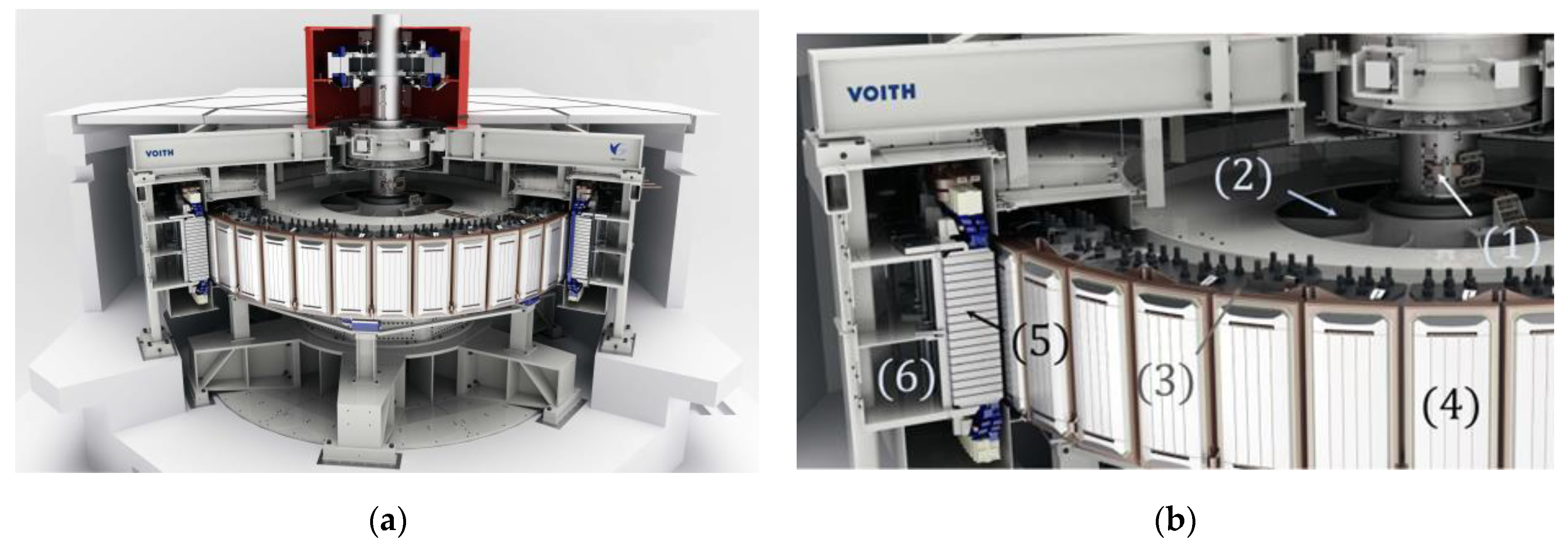
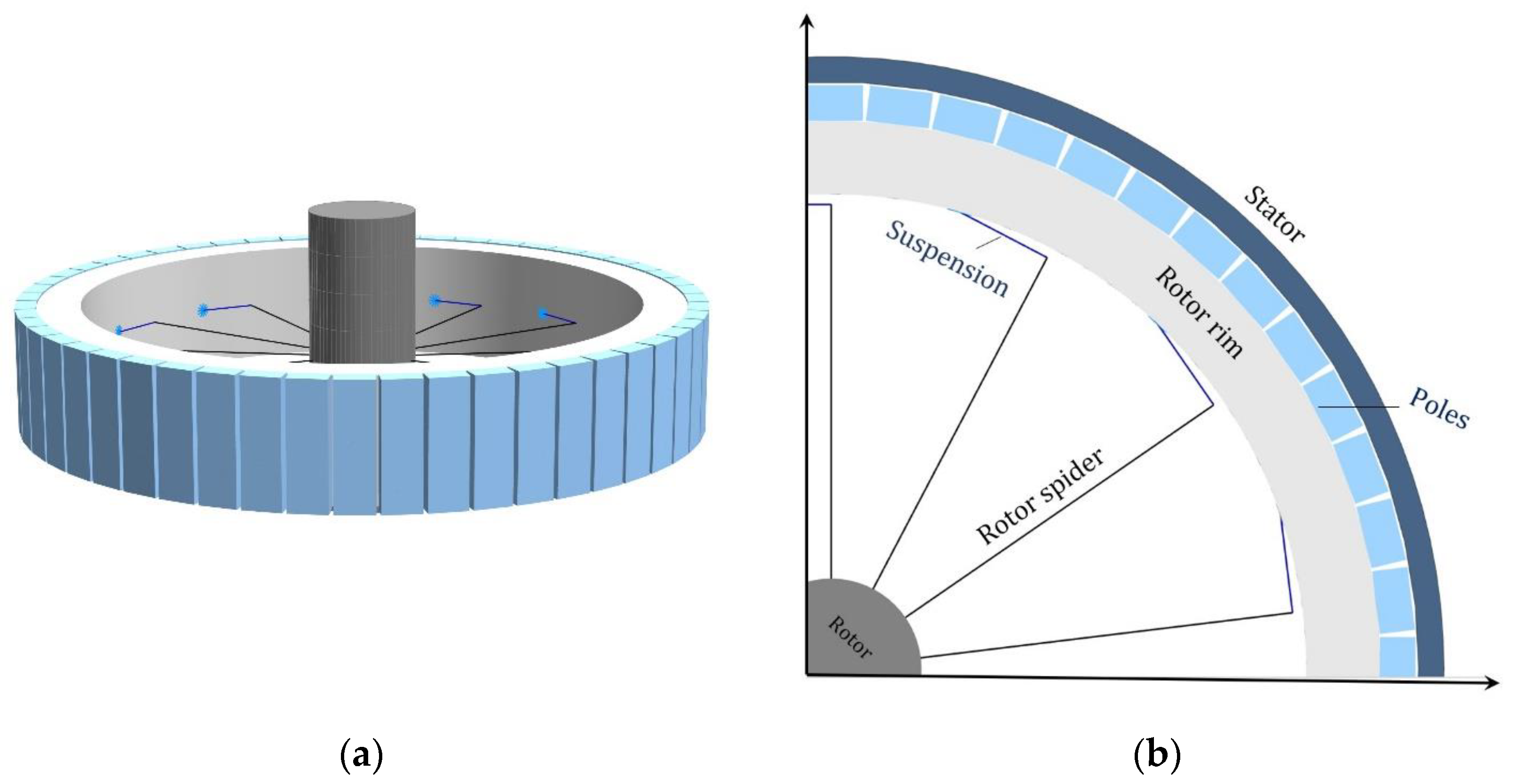
A 190 MW hydropower generator–rotor system was modeled using Finite Elements. Eigenvalue and transient response analyses were performed using the Simcenter Nastran 2212.0 solvers 414-110 and 414-129, respectively. A model of a hydropower generator is shown in Figure 1; comprehensive illustrations of the rotor and stator can be found in Gustavsson et al. (2012) [19]. For the purpose of this article, the rotor and stator’s geometry was idealized, and a simplified rotor and stator system model is illustrated in Figure 2a. The studied system comprises five main components, namely the rotor rim, rotor spider, poles, rotor shaft, and stator, as shown in Figure 2b.

2.1. Rotor Rim

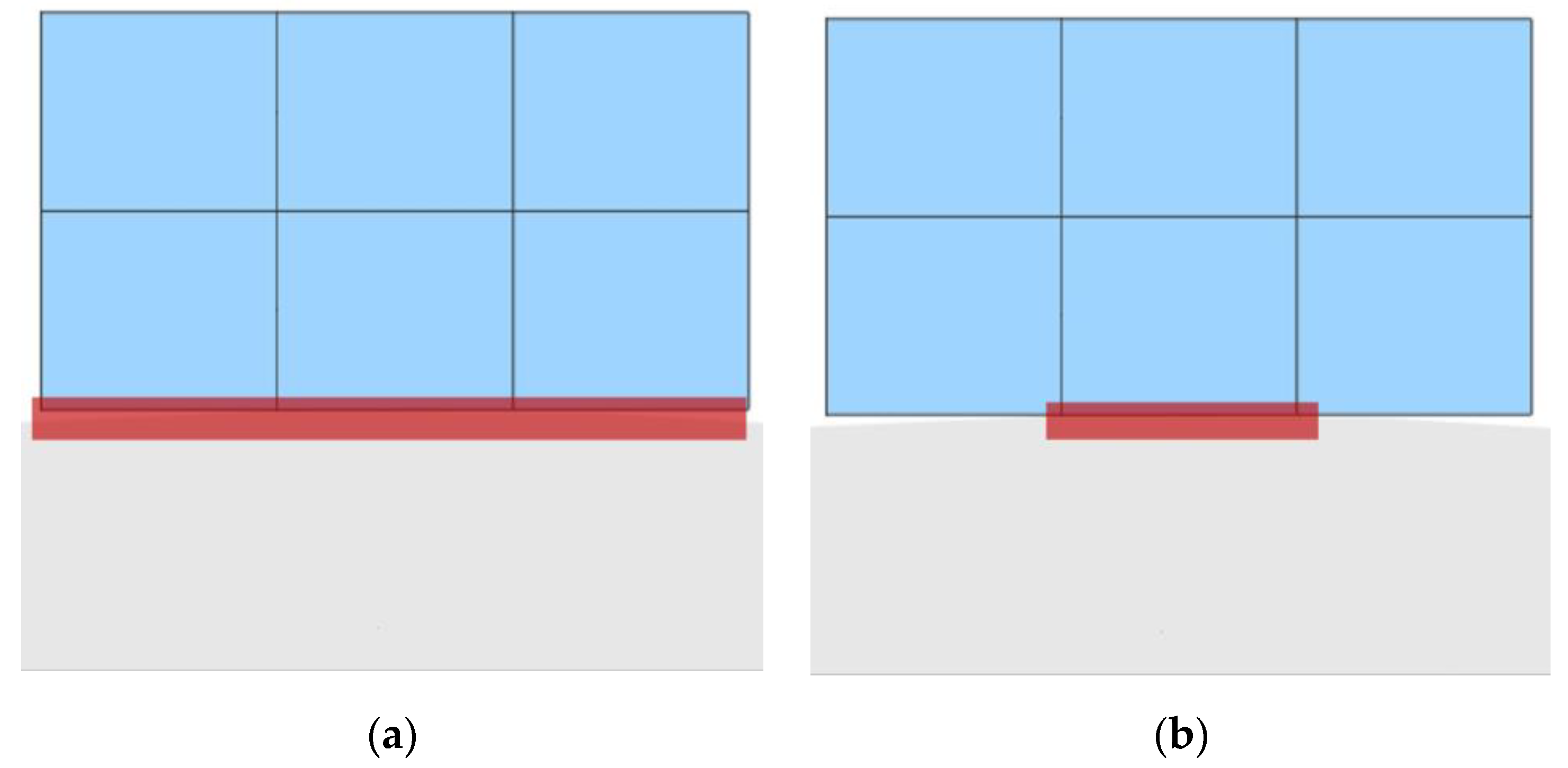
The generator rim is discretized by 21,236 ten-node tetrahedral elements and is modeled as isotropic, linear elastic steel with the material properties defined in Rondon et al. (2023) [20]. The outer surface of the rim connects to the poles. The connection is made of constraining boundary nodes at the pole–rim interface. To enable the connection between dissimilar meshes, the constrained nodes are identified by the distance between the target bodies (the poles) and the source bodies (the rim). As the rim surface is circular and the pole surface is rectangular, the number of participating nodes in the connection is affected by the distance. A shorter distance will only reduce the pole width, while a longer distance will increase the whole pole width. Figure 3a,b show examples of the different possible bonds along the pole width. Note that the node participation can also vary along the pole length.

2.2. Poles

All 52 poles are comprised of a total of 3432 twenty-node hexaeder elements evenly distributed along the circumference of the rotor rim.

A radial magnetic pull is generated as the output of the spring-damper element, which produces a force based on the distance between the stator node and the auxiliary node created at the centroid of the pole surfaces. The radial force has a constant component and one component that varies linearly with the distance between the poles’ and the stator’s surfaces, as described in Rondon et al. (2023) [20]. On the other hand, tangential magnetic stiffness is applied to the same spring-damper element, albeit in the circumferential direction of the pole surface.

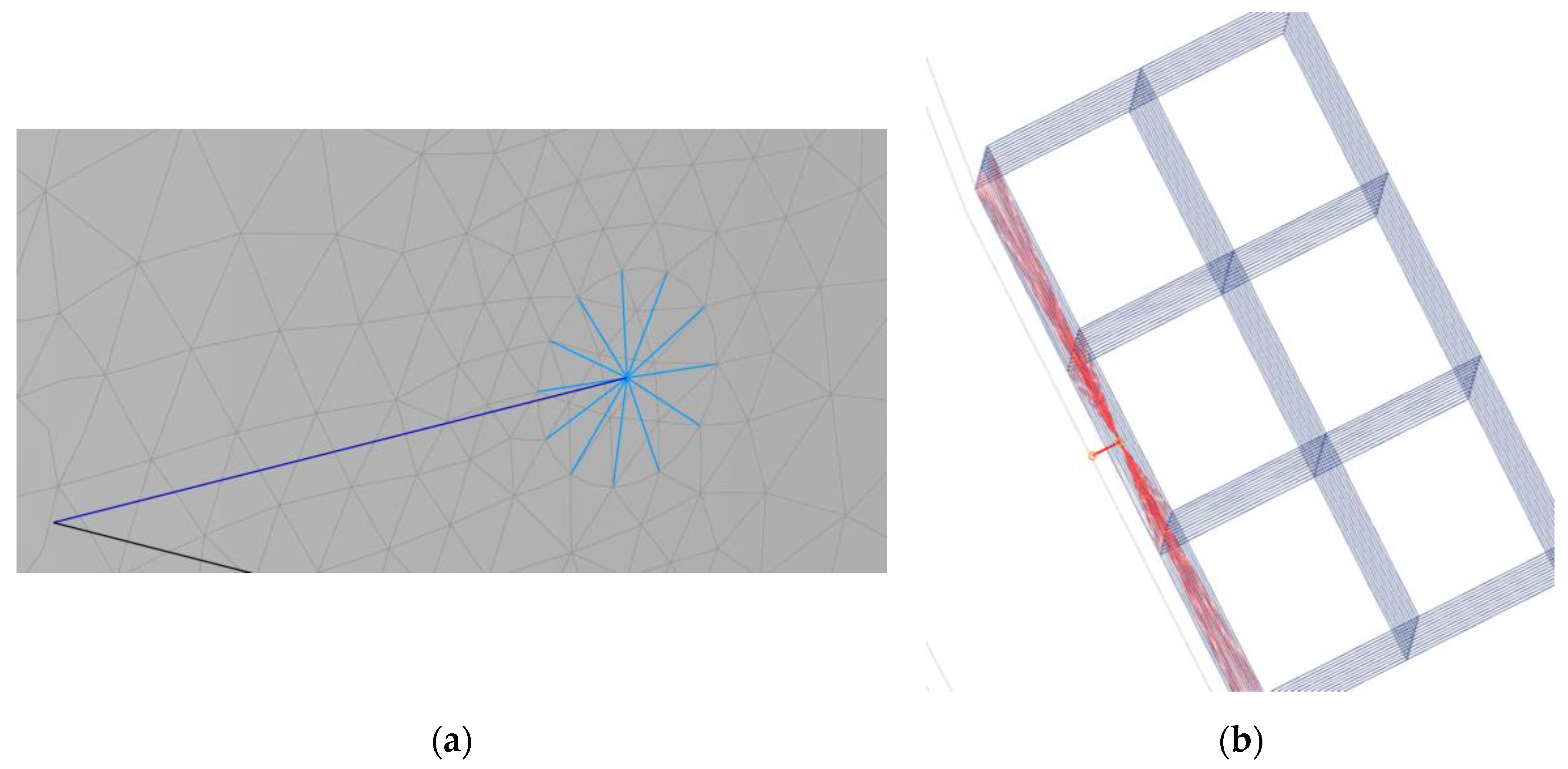
A spider element (multi-point constraint) distributes the effects of radial magnetic pull from the auxiliary node to the pole nodes. In contrast to the spider elements utilized for the rotor spider, the element constraint does not represent a kinematic constraint. The displacement of the auxiliary node was computed as a weighted average of the motion of the pole surface nodes. This enables relative motion between the nodes of the pole surface and, thereby, no excessive stiffening occurs. Figure 4b shows how the interpolation element (red) connects the auxiliary node to the pole surface nodes.

2.3. Rotor Spider

The rotor spider system consists of the main structure and the elements connected to the rotor rim. The rotor spider’s structure is modeled as a single spider element, i.e., a kinematic multi-point constraint that enforces a rigid connection between a single independent node and several dependent nodes (see Figure 4a). The dependent nodes are connected to the rotor rim by spring-damper elements, while the independent node is the center node of the rotor. Thus, the rotation and translation of the independent node fully define the translation of dependent nodes. The rotor spider structure merely serves as the base of the spring-damper elements without contributing to the system’s dynamics.

The rotor rim suspension consists of 13 generalized spring-damper elements evenly distributed along the rotor rim’s inner circumference, connected to the rotor rim’s inner surface by single-spider elements. The generalized spring-damper elements allow for the input of tri-axial stiffness and damping according to a locally defined coordinate system.

2.4. Rotor-Bearing System

The rotor shaft is discretized by eight Timoshenko beam elements. A general mass element is utilized on the center node to represent the combined inertial properties of the shaft and rotor spider. This center node is connected to the rotor spider by a spider element. The rotor shaft is constrained to movements in the axial direction.

The bearing elements are connected at each end of the rotor shaft; their properties are defined in Rondon et al. (2023) [20]. Each bearing element connects two nodes: a moving node on the shaft axis and a coincident node fixed to the rotating frame.

2.5. Stator

The stator is represented by 52 massless nodes with every degree of freedom fixed to a rotating frame. The spring-damper element utilizes the position of the fixed stator node to determine the magnitude of radial magnetic pull.

Indeed, the use of a rotating stator does not reflect physical machinery but restricts analysis to a single frame of reference, effectively simplifying the mathematical formulation. For a rigid, axisymmetric stator, monitoring an individual pole–stator distance merely involves comparing the time-dependent pole coordinate to a fixed radial coordinate, valid regardless of the stator’s angular orientation.

This justifies the choice to fix the stator to a rotating frame of reference rather than to involve two different frames of reference. However, this additional complexity is necessary to achieve interaction with a non-axisymmetric stator.

2.6. Boundary Conditions

The boundary conditions consist of fixing the stator nodes and the bearing nodes to the rotating frame. The fixed bearing nodes are coincident with the axis of rotation.

3. Theoretical Background

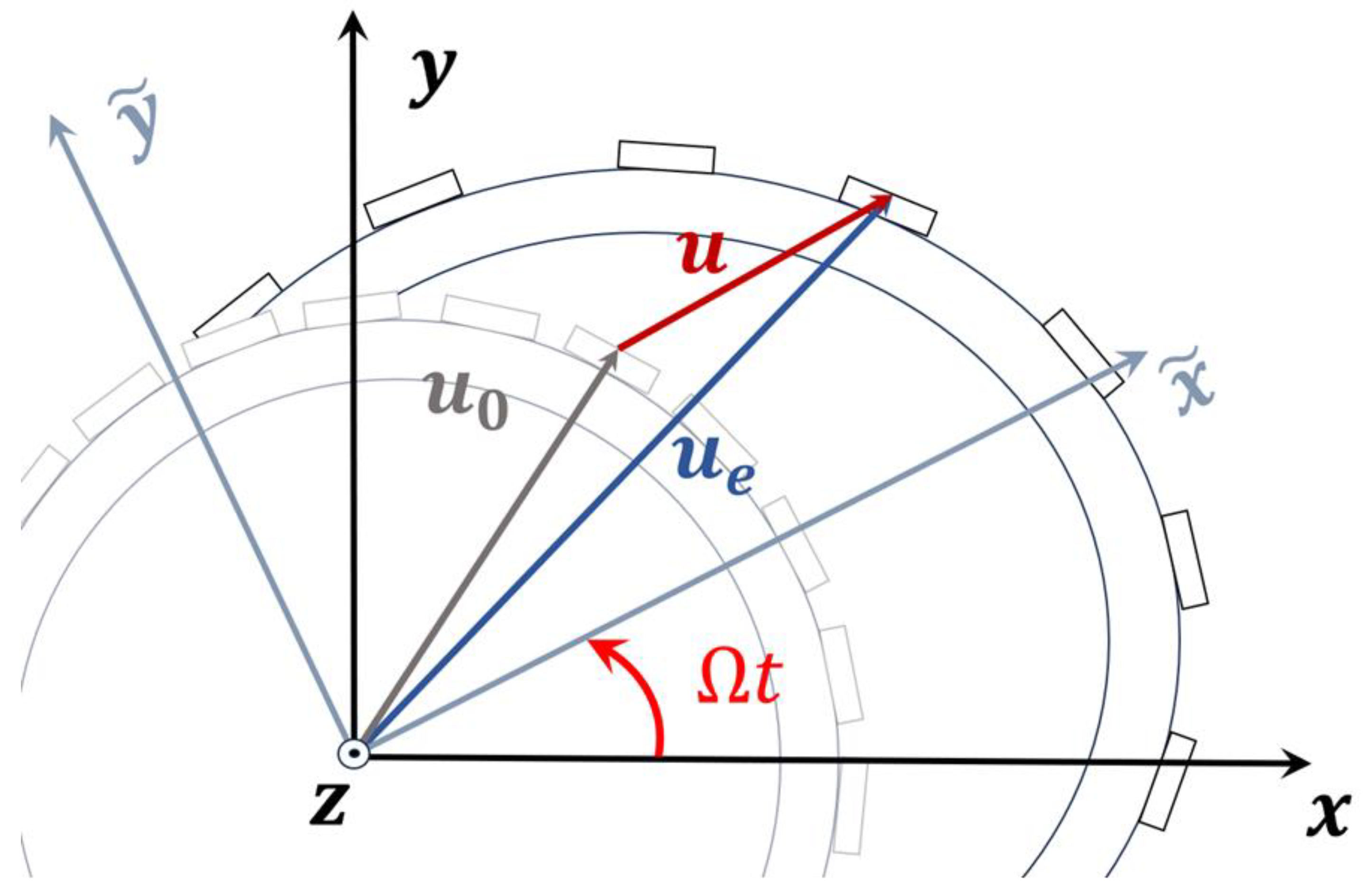
Consider the three-dimensional rotor system of the generator depicted in Figure 2b, which is defined by its radial, tangential, and axial coordinates, according to Figure 5. The rotating radial–tangential coordinate system with radial, tangential, and axial directions (denoted as $\tilde{\mathit{x}}, \widetilde{\mathit{y},} \mathit{z}$, respectively) rotates at a synchronous speed Ω. The nodes are initially located at the position ${\mathit{u}}_0$ and elastically deformed to the absolute position ${\mathit{u}}_{\mathit{e}}\left(t\right)$ due to the external load $\mathit{F}\left(\mathsf{\Omega },t\right)$, resulting in relative displacement $\mathit{u}\left(t\right)$.

Consider the following equation of motion for the system under the influence of time- and speed-dependent forces:

$$\mathbf{M}\ddot{\mathit{u}}\left(t\right)+\left(2\mathsf{\Omega }\mathbf{C}+\mathbf{D}\right)\dot{\mathit{u}}\left(t\right)+\left(\mathbf{K}-{\mathsf{\Omega }}^2\mathbf{Z}\right)\mathit{u}\left(t\right)=\mathit{F}\left(\mathsf{\Omega },t\right),$$

(1)

where $\mathbf{M}$ represents the inertial matrix, which is calculated from the discretized geometry. The term C includes Coriolis effects arising due to analyzing the system in a rotating frame of reference. D denotes the external viscous damping matrix produced by, i.e., the bearing damping. $\mathbf{K}$ represents the stiffness matrix, incorporating the combined elasticity of the shaft, bearings, and connecting elements, as well as the three-dimensional discretization of the rotor rim and poles. $\mathbf{Z}$ denotes the centrifugal softening matrix also arising due to the utilization of a rotating frame of reference.

3.1. Centrifugal Loads

The force $\mathit{F}\left(\mathsf{\Omega },t\right)$ involves centrifugal loads and Unbalanced Magnetic Pull. Centrifugal forces act on the radial subset of the global displacement vector ${\mathit{u}}_{0,r}$ according to the following equation:

$${\mathit{F}}_{\mathbf{c}}={{\mathsf{\Omega }}^2\mathbf{M}}_r{\mathit{u}}_{0,r},$$

(2)

where ${\mathbf{M}}_r$ represents a sub-matrix from the global inertial matrix, only concerning the mass at the radial degrees of freedom.

3.2. Unbalanced Magnetic Pull

Unbalanced Magnetic Pull is modeled as a linear formulation governed by the radial distance between the pole and stator, which is formulated as follows:

$${\mathit{F}}_m=k_m\left({{\mathit{u}}_{e,r}}^{\mathrm{P}}-{{\mathit{u}}_{\mathit{e},r}}^{\mathrm{S}}\right)+{\mathit{F}}_{0,m}$$

(3)

where ${{\mathit{u}}_{e,r}}^{\mathrm{P}}$ and ${{\mathit{u}}_{\mathit{e},r}}^{\mathrm{S}}$ represent subsets of ${\mathit{u}}_{\mathit{e}}$ concerning the absolute position of the pole nodes and the stator nodes (superscripts P and S, respectively). ${\mathit{F}}_{0,m}$ denotes the magnetic preload and describes a pull directed radially outward. $k_m$ represents the scalar magnetic stiffness.

4. Results and Analysis

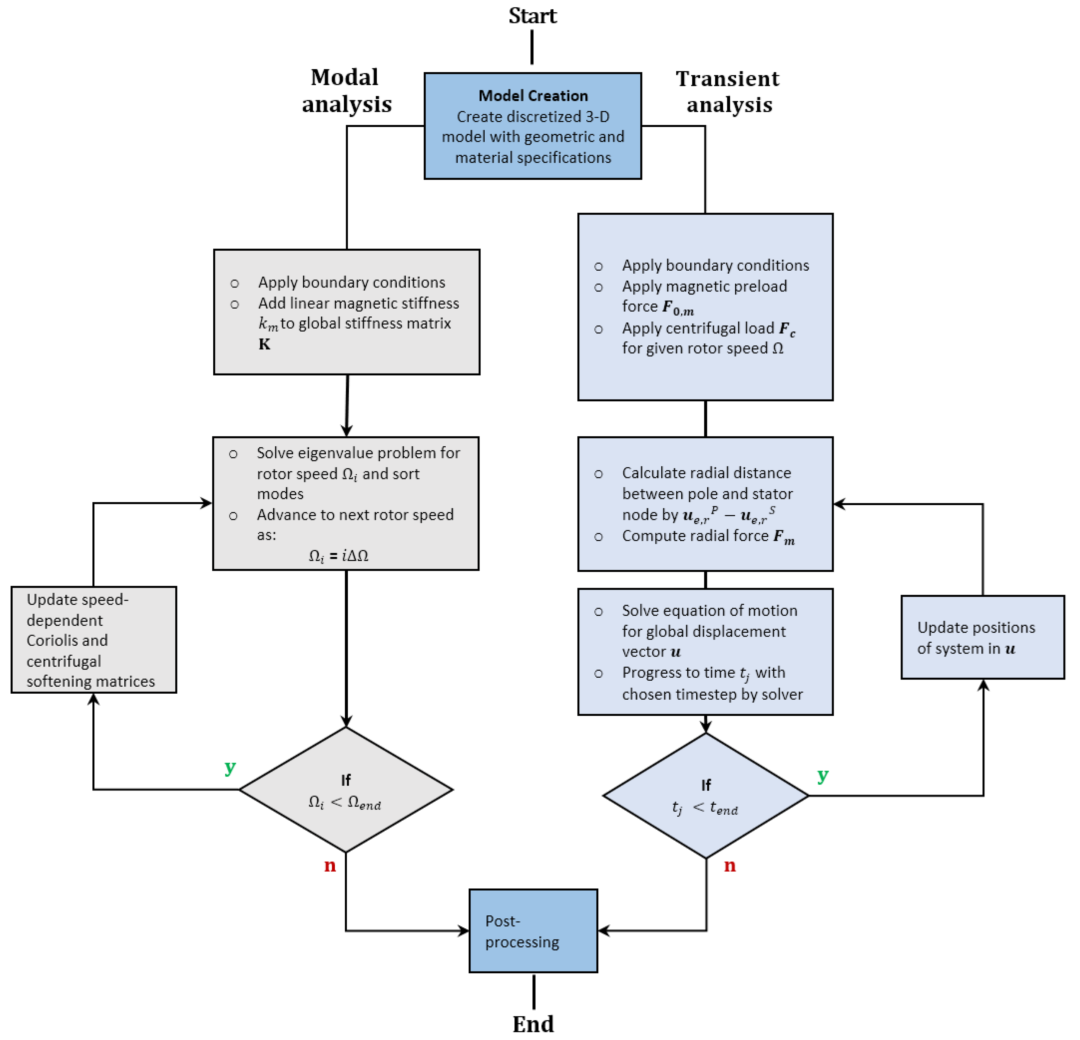
Modal and transient analyses were conducted on the three-dimensional model of the generator using the procedure illustrated in Figure 6. Modal analysis was utilized to determine the eigenvalues and modes of the generator, focusing particularly on the influence of the plates and poles. In contrast, transient analysis was performed to assess the rotor rim’s expansion, considering the impacts of centrifugal and electromagnetic forces.

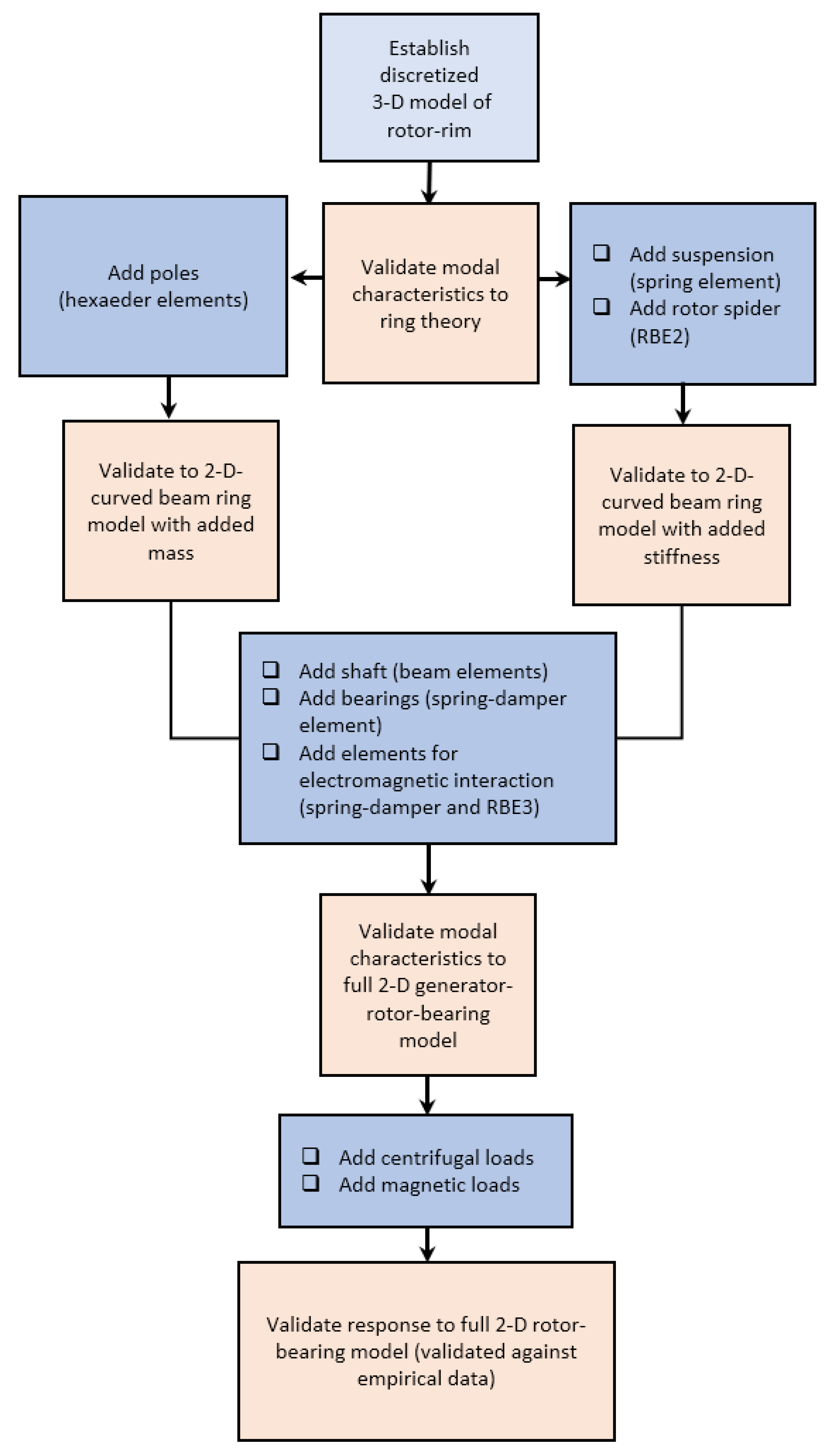
The validation of this model starts with performing the modal analysis of the rotor rim and contrasting the results to those of the ring theory using the model in Lin and Soedel (1988) [26], and the 2-D curved beam model, which were validated against empirical data. After the eigenvalues and modes were compared, the influence of the plates and poles was also studied independently. Afterward, modal analysis was performed on the model, including the influence of the plates, poles, and electromagnetic interaction, comparing the results to those of the 2-D curved beam model. Lastly, by adding the centrifugal and electromagnetic loads, the models were compared via transient analysis. A flowchart of these procedures is illustrated in Figure 7.

4.1. Eigenvalues and Modes

The model was tested in steps, from analyzing the free ring, the contribution of poles, and the connection plates to comparing the 2-D and 3-D models with and without the influence of electromagnetic forces.

4.1.1. Free Ring

Comparing the results from the 3-D and 2-D models to the eigenvalues estimated using the ring theory (shown in

Table 1. Comparison of the natural frequencies of the free ring theory, 2-D, and 3-D models.

Modes	Ring Theory from [26]	2-D Model from [20]	3-D Model
1st Bending	15.97	15.68	15.71
2nd Bending	45.17	43.86	43.82
3rd Bending	86.62	82.23	86.10
4th Bending	140.08	128.50	130.11
Expansion	143.62	143.34	142.43
5th Bending	205.49	182.61	185.70

) shows that they are very similar, with most deviations below 10% for the 3-D model and 12% for the 2-D model. In general, the results from the 3-D model are more accurate to the theory. The main trend of the results is that the errors increase with the mode order, with the outlier being classified as the third bending mode, where the 3-D model estimate is below 1% error, while that of the 2-D model using curved beams is 5.3%.

4.1.2. Influence of Poles

The overall consequence of adding connecting plates between the rotor rim and the rotor spider is that they stiffen the system, at least for the first two bending modes, with 41.9% and 5%, respectively. The rest of the eigenvalues show a decrease from the free-ring ones, though they are less than 3.5%. Adding the rotor spider and the plates also introduces more modes of vibrations; this is noted in

Table 2. Comparison of the influence of connecting plates on the natural frequencies of the rotor rim using 2-D and 3-D models.

Mode	2-D Model from [20]	3-D Model
Overdamped	0.00	0.00
1st Torsion	7.70	7.80
1st Bending	21.09	22.30
Counter-lateral	21.63	21.10
2nd Bending	44.82	46.01
3rd Bending	79.34	83.08
4th Bending	117.71	129.94
Expansion	127.99	140.92
2nd Torsion	128.15	118.39
5th Bending	149.62	184.81

. In general, the 3-D model overestimates the natural frequencies with respect to the 2-D model with curved beams, from 1.4% in the first torsion mode to 23.5% in the fifth bending mode.

4.1.3. Influence of Connecting Plates

In contrast to the influence of connecting plates, adding poles to the system reduces the natural frequencies of the free ring. The effect is similar in the 2-D and 3-D models, where this decrease accounted for between 14 and 19% of the free-ring frequencies, as shown in

Table 3. Comparison of the influence of poles on the natural frequencies of the rotor rim using 2-D and 3-D models.

Modes	2-D Model from [20]	3-D Model
Overdamped	0.00	0.00
1st Torsion	6.52	6.76
1st Bending	13.34	13.46
2nd Bending	35.94	37.17
3rd Bending	66.68	69.18
4th Bending	103.88	107.61
Expansion	119.15	115.51
5th Bending	146.23	150.79

. Comparing the 2-D and the 3-D model frequencies, the natural frequencies of the former and those corresponding to the expansion modes are the exceptions, which increase by 3%.

4.1.4. Full Model

In

Table 4. Comparison of the natural frequencies of the rotor using 2-D and 3-D models. Part 1.

2-D Model					3-D Model
Mode	No Magnetic Stiffness		Magnetic Stiffness		No Magnetic Stiffness		Magnetic Stiffness		Mode
	0 Hz	50 Hz	0 Hz	50 Hz	0 Hz	50 Hz	0 Hz	50 Hz
	0.00	0.00	0.00	0.00	0.00	0.00	0.00	0.00
	6.43	6.14	6.43	6.14	6.92	6.85	6.92	6.85
	17.45	15.90	15.52	13.97	19.05	17.50	17.00	16.04
		18.92		16.98		20.65		18.95
	17.95	16.05	16.77	14.86	17.02	15.07	15.78	13.89
		19.86		18.67		18.70		17.74
	36.65	35.50	35.70	34.55	39.20	38.70	38.32	37.81
		37.74		36.79		40.39		39.50

and

Table 5. Comparison of the natural frequencies of the rotor using 2-D and 3-D models. Part 2.

2-D Model					3-D Model
Mode	No Magnetic Stiffness		Magnetic Stiffness		No Magnetic Stiffness		Magnetic Stiffness		Mode
	0 Hz	50 Hz	0 Hz	50 Hz	0 Hz	50 Hz	0 Hz	50 Hz
	65.52	64.62	65.02	64.13	70.20	70.21	69.76	69.71
		66.37		65.87		71.00		70.58
	98.33	97.61	98.04	97.32	108.30	108.60	108.00	108.28
		99.02		98.74		108.84		108.52
	110.50	110.55	110.23	110.28	115.40	115.47	115.00	115.15
	127.51	127.51	127.51	127.51	117.50	117.53	117.50	117.53
	129.94	129.35	129.79	129.19	151.30	151.60	148.70	151.63
		130.53		130.37		151.85		151.60

, the eigenvalues for the 2-D and 3-D models were compared at a standstill and during 50 Hz rotation, with and without the effects of magnetic pull. At a standstill, the 3-D model estimated higher natural frequencies than the 2-D model did in most cases, with maximum deviations in the fifth bending mode of 16.4% with no magnetic pull and 14.6% with magnetic pull. At 50 Hz, this deviation increased to a maximum of 17.4% with and without magnetic pull; the exceptions are the counter-lateral and second torsion modes, where the 3-D model underestimated the natural frequencies by a maximum of 7.8%.

The eigenvalues are also similar under a magnetic influence; at 0 Hz (standstill), the difference with and without magnetic pull varies consistently, with a variation of 11% in the first bending mode in the 2-D model and 10.8% in the 3-D model. This difference decreases for both the models at the higher modes. Upon increasing the frequency to 50 Hz, the models begin to exhibit divergent behaviors; a maximal difference of 12.2% is observed in the 2-D model, contrasting with a smaller 8.3% in the 3-D model. As the higher modes are examined, the discrepancies between the two models tend to align more closely.

In the first round of torsion mode analysis, the natural frequency exhibits varied responses at different speeds in the 2-D and 3-D models. For the 2-D model, an appreciable decrease in natural frequency is observed as the rotation speed changes, from 6.43 Hz at a standstill (0 Hz) to 6.14 Hz when the rotation speed reaches 50 Hz. In contrast, the natural frequency in the 3-D model remains constant at 6.83 Hz, irrespective of the rotation speed.

The bending modes in the forward and backward directions are due to Coriolis forces acting on the ring, as evidenced by the split at 50 Hz, which is in agreement with Rondon et al. (2023) [20].

4.2. Rotor Rim’s Expansion

To evaluate the radial displacement of poles using the 2-D and 3-D models, three sets of poles were chosen for analysis; poles 1, 17, and 37 correspond to the pole positions directly affected by the connection plates, while the other poles in the set correspond to the adjacent pole positions.

Table 6. Comparison of the radial displacement of poles with and without magnetic force using 2-D and 3-D models. Pole positions where the suspension plates are connected to the rotor rim are denoted in bold.

		No Magnetic Force		Magnetic Force
		2-D Model from [20]	3-D Model	2-D Model from [20]	3-D Model
Set 1	Pole 51	1.087	0.967	1.166	1.094
	Pole 52	1.087	0.965	1.166	1.092
	Pole 1	1.087	0.964	1.166	1.091
	Pole 2	1.087	0.965	1.166	1.093
	Pole 3	1.087	0.969	1.166	1.097
Set 2	Pole 15	1.087	0.973	1.166	1.103
	Pole 16	1.087	0.976	1.166	1.106
	Pole 17	1.087	0.978	1.166	1.108
	Pole 18	1.087	0.978	1.166	1.108
	Pole 19	1.087	0.978	1.166	1.106
Set 3	Pole 35	1.087	0.986	1.166	1.116
	Pole 36	1.087	0.985	1.166	1.116
	Pole 37	1.087	0.984	1.166	1.115
	Pole 38	1.087	0.979	1.166	1.108
	Pole 39	1.087	0.974	1.166	1.103

compares radial expansion for the 2-D and 3-D models with and without the influence of the magnetic forces. Without magnetic forces, the rotor rim expands due to the influence of the centrifugal forces of the pole and rim’s masses; the 3-D model underestimates the radial expansion by an average of 10.3% with respect to the 2-D model, with no clear difference between the poles linked to the plates and the adjacent poles. However, the magnetic forces appear to have a greater influence in the 3-D model as the deviation is halved. This difference is clearer when comparing the increase in expansion due to magnetic forces for the 2-D model from 7.3% to 13.2% in the 3-D model. This difference can be explained as the result of assuming the poles at the rotor as flexible in contrast to the 2-D model where the poles are assumed to be rigid, and the connection between the centerline and pole node is also rigid.

5. Discussion

It is important to acknowledge the challenges in obtaining empirical data; manufacturers and operators of hydropower generators do not typically disclose detailed measurements of their units. This lack of accessible data presents a considerable obstacle in obtaining the accurate and specific parameters needed for validation. Additionally, constructing test rigs to simulate the operational conditions of these generators is a time-intensive process. Alternatively, the 2-D model from Rondon et al. (2023) was used to validate this model.

One of the main differences between the 3-D model in the FEM and the 2-D model is the discretization of the rotor rim. While the model using curved beam elements depends on the number of poles, the 3-D Finite Element model is more complex. The rim is comprised of 34,222 nodes distributed among ten-node tetrahedral elements, with three degrees of freedom per node. The element utilizes grid points for both the edge points and midpoints along the element vertices, enabling the use of relatively few elements in the radial direction. The three-dimensional discretization of the rotor rim serves several purposes. It enables the simultaneous study of both in- and out-of-plane vibrations, as well as coupling between these. Furthermore, it also captures the shear deformation that can occur for thick rings, i.e., where the radial displacement is not uniform throughout the vertical direction in the ring.

In contrast to the 2-D model, the poles are discretized by three-dimensional elements to reflect their actual geometry and are not assumed to be stiff. The poles are discretized by hexahedral elements with 20 nodes per element. The connection between the rotor rim and the poles is made by constraining the surface nodes of the pole to the surface nodes of the inner rotor rim; see Figure 3a,b for an illustration. By including the geometry of the poles, the 3-D model demonstrates that the magnetic interaction is distributed over the pole surface rather than acting at a single node.

The connection between the poles and rim introduces stiffening effects. As the constraint connection between the poles and rim is fully rigid, the poles effectively act as an additional layer of material in the radial direction; hence, they are a structural element. Table 3 shows that the natural frequencies in the 3-D model are higher than those of the 2-D model, with an average of 2.5%, especially comparing this deviation to the results for the free-ring simulations, with an average of 0.7%. It is noted that the participating pole surface can be varied to simulate varying degrees of rigidity in the connection, but for this paper, the full bond along the pole length is utilized for the constraint. However, whether this is the optimal way to model physical connections between components has not been determined.

The connection plates also work differently in the models. In the 2-D model, the rotor rim nodes are at the centerline; thus, the plates are in direct contact with them. Meanwhile, in the 3-D model, the plates are connected to a finite number of nodes at the inner radius of the rotor rim using a spider connection (see Figure 4a). Thus, the connecting elements distribute forces within a limited area of the inner rim surface but also with a considerable radial offset to the centerline of the rim.

6. Conclusions

This study explored different approaches to modeling a hydropower generator with a floating rotor rim by comparing a 3-D model using the FEM with a 2-D model using the curved beam elements proposed by Rondon et al. (2023) [20] and validated using the measurements in Gustavsson et al. (2012) [19]. Several conclusions can be drawn from this comparison as follows:

• The 3-D model is more complex than the 2-D model due to discretization and the type of element employed, resulting in the appearance of both in-plane and out-of-plane modes of vibrations. The 2-D model, in contrast, is comprised of curved beam elements with a significantly smaller number of elements. However, the analysis concludes that the natural frequencies in both models are similar, with most of the deviations being below 10%.
• Pole discretization in the 3-D model introduces stiffening effects on the model because the poles act like additional structural elements, increasing the natural frequencies. This also increases the radial expansion of the rotor in contrast to that of the 2-D model.
• The connecting plates work differently in the two models; in the 3-D model, the plates are connected to the inner radius of the rotor rim using spider connections, distributing the forces to a limited area, while the plates in the 2-D model are connected directly to the nodes at the centerline of the rotor. This difference can also affect the natural frequencies and transient performance results.

In general, the proposed model can estimate the deformation and natural frequencies of a rotor in a generator, providing valuable information to designers and manufacturers. Modeling the dynamic contributions of geometry confined to three dimensions is crucial, which enables the characterization of dynamic properties for complex, elastic mechanical systems. This capacity also facilitates the analysis of complex loading scenarios while including the possibility of assessing the influence of detailed geometry for, e.g., stress evaluation and fatigue analysis.