Weak Signal Extraction in Noise Using Variable-Step Gaussian-Sinusiodal Filter

Abstract

When analyzing vibration or acoustic signals in machinery, noise interference within the characteristic signals can significantly distort the results. This issue is particularly pronounced in complex environments, where mechanical signals are often overwhelmed by noise, making it extremely difficult or even impossible to determine the operational status of mechanical equipment by the analysis of characteristic signals. Existing methods for analyzing weak signals in the presence of strong Gaussian noise have limitations in their effectiveness. This paper proposes an innovative approach that utilizes a Variable-Step Gaussian-Sinusoidal Filter (VSGF) combined with rotational coordinate transformation to extract weak signals from strong noise backgrounds. The proposed method improves noise reduction capabilities and frequency selectivity, showing significant improvements over traditional Gaussian filters. Experimental validation demonstrates that the signal detection accuracy of the proposed method is 10–15% higher than that of conventional Gaussian filters. This paper presents a detailed mathematical analysis, experimental validation, and comparisons with other methods to demonstrate the effectiveness of the proposed approach.

1. Introduction

With advancements in the mechanical manufacturing industry, engineering machinery has become increasingly precise, leading to higher demands for predicting and detecting mechanical faults. In complex operating environments, the high noise content in mechanical signals often obscures characteristic signals, resulting in a very low signal-to-noise ratio (SNR). This makes fault diagnosis particularly challenging. To accurately analyze mechanical signals and address the issue of weak signal analysis, extensive research has been conducted. These methods can be broadly categorized into two types: noise-reduction-based signal analysis methods and stochastic resonance methods that utilize noise.

Noise-reduction-based signal analysis methods primarily include the following: 1. Statistical measurement methods: Metrics such as mean, variance, and standard deviation are calculated to mitigate the impact of noise. 2. Autocorrelation function: The correlation between the signal and its delayed version is measured to identify repeating patterns or periodic components. 3. Time domain filters: Low-pass, high-pass, or band-pass filters are used to isolate specific frequency components.

Martínez [1] proposed a wavelet-based electrocardiogram (ECG) signal analysis method that combines statistical measurements to assess ECG signal characteristics, demonstrating superiority in detecting QRS complexes. Smith [2] diagnosed rolling element bearing faults using the autocorrelation function and adaptive noise cancellation techniques, showcasing the efficacy of autocorrelation analysis in practical applications. Antoni [3] analyzed non-stationary vibration signals using time domain filters, introduced the concept of spectral kurtosis and demonstrated the advantages of time domain filtering in signal feature extraction. Hu [4] introduced a novel chaotic system aimed at improving the signal-to-noise ratio (SNR) in complex noise environments. The study showed that this chaotic system outperformed traditional noise reduction methods, making it a promising tool for handling nonlinear and complex background noise. Zhang and Yang [5] proposed an adaptive Gaussian filtering method for signal denoising, which adjusts the filter’s standard deviation according to different noise levels. This approach allows for a more effective noise reduction while preserving important signal details, significantly improving overall denoising performance. With the development of filters, space-variant Gaussian filters have also been applied in image processing. Mäkitalo and Foi [6] developed these filters, which adjust their parameters based on different regions of the image, effectively managing noise while preserving critical details and improving image quality. Y. Wang [7] focused on designing adaptive filtering methods for detecting weak signals in high-noise environments. By continuously adjusting the filter parameters based on the received signal, this method effectively improved the signal-to-noise ratio, making it easier to identify weak signals. S. Haykin [8] authored a classic textbook in the field of adaptive filtering, covering the theory and application of various adaptive filtering algorithms. It provides a thorough explanation of how these filters can be used to reduce noise and enhance the clarity of weak signals in complex environments. M. G. Bellanger [9] offers a comprehensive introduction to digital signal processing, with a particular focus on filtering techniques. It includes detailed explanations of how different filters, including adaptive filters and Gaussian filters, are applied to noise reduction and weak signal enhancement. X. M. Li and J. F. Zhou [10] explored the use of Ensemble Empirical Mode Decomposition (EEMD) to detect faults in bearings. This method is particularly adept at extracting weak fault signals from noisy vibration data, making it a valuable tool in the condition monitoring of rotating machinery.

Stochastic resonance (SR) has been recognized as a powerful tool for weak signal detection, particularly in nonlinear systems. The theory of stochastic resonance was initially systematized by Benzi [11], who demonstrated how noise could enhance the detection of weak periodic signals in nonlinear systems. This foundational work laid the groundwork for the application of SR in various fields, including mechanical fault diagnosis. Hou [12] explored the use of stochastic resonance for signal detection in colored noise environments and demonstrated its effectiveness in signal enhancement. McNamara and Wiesenfeld [13] further elaborated on the fundamental theory and physical mechanisms of SR, demonstrating through mathematical derivations and experiments how the introduction of an appropriate amount of noise can enhance weak signal detection. This work had a significant impact on subsequent research and the practical application of SR in various fields. Building on this, Barbini [14] studied the application of a two-dimensional SR method, which outperformed traditional one-dimensional methods in detecting weak signals in complex noise environments. This method has shown great potential in fields such as image processing and signal detection. In practical applications, Liu [15] applied SR technology to bearing fault diagnosis, a critical aspect of mechanical fault detection. Their method effectively amplified weak vibration signals, enabling early and accurate fault detection, which is crucial for mechanical maintenance and reliability. Shu-Yao [16] further explored the application of SR in underwater acoustic weak signal detection, where complex and variable noise challenges exist in the underwater environment. By combining SR technology, the study significantly improved the detection performance of underwater weak signals, demonstrating its practical potential. Finally, the combination of SR with other advanced methods, such as chaotic systems, has shown promise in enhancing weak signal detection. Liu [17] proposed an approach that integrates SR and chaotic systems, utilizing the complex dynamic behavior of chaotic systems to enhance weak signals in noise. This integration has shown potential in real-world signal processing, particularly in nonlinear environments. M. I. Ribeiro and M. V. de Freitas [18] explored the application of wavelet transforms in detecting weak signals masked by chaotic noise. The paper discusses the advantages of wavelet analysis in decomposing signals into different frequency components, which enhances weak signals initially obscured by chaotic dynamics. F. K. Gruber [19] introduced a new method for reducing noise in nonlinear systems by leveraging chaotic behavior. The paper demonstrates how chaotic dynamics can be utilized to filter out noise, improving the detection of weak signals. This approach is particularly useful in systems where traditional linear methods fail. G. Parisi [20] provided a comprehensive theoretical framework describing the phenomenon of stochastic resonance, where noise can actually enhance the detection of weak signals. The author supports their theory with experimental results, demonstrating the practical application of stochastic resonance in various physical and biological systems. L. Y. Chen [21] discussed the use of wavelet transforms to detect faults in mechanical systems, particularly in cases involving weak signals. The paper demonstrates how wavelet-based methods can isolate signal features indicative of faults, even when these features are obscured by noise. E. W. Bai [22] introduced a chaos-based filter specifically designed for detecting weak signals in noisy environments. The author explains the mathematical foundations of chaotic filtering and provides examples of its application in signal processing tasks where traditional filters perform poorly. H. Kantz [23] authored a book that covers the analysis of nonlinear time series, applied to chaotic systems and signal detection. It includes methods for identifying weak signals under complex nonlinear behavior in data, providing tools for both theoretical understanding and practical application. R. H. Brown [24] proposed a neural network-based approach for noise suppression and weak signal detection. The paper details how neural networks can be trained to distinguish between noise and signal, effectively enhancing weak signals in complex environments. J. J. Benedetto [25] explored the application of wavelet transforms and time–frequency analysis for weak signal detection. The paper emphasizes how these methods provide a detailed analysis of signal components at different scales and frequencies, making them well suited for noise suppression and weak signal enhancement. G. T. Reed [26] explored the application of stochastic resonance to enhance weak signals in fiber optic communication systems. The author demonstrated how noise could be utilized to improve the detection of weak signals, which is particularly useful in optical networks. S. Mallat [27] authored a comprehensive guide on wavelet transform techniques in the field of signal processing. It covers wavelet transform theory and applications, including noise suppression, signal compression, and weak signal enhancement, making it an essential resource for researchers in this field.

While the aforementioned methods have contributed to weak signal detection, some of them suffer from limitations such as low detection accuracy or cumbersome application processes. Therefore, to accurately analyze the characteristics of weak signals in complex and dynamic environments, especially for the extraction and analysis of weak signals from strong noise backgrounds, this paper introduces a Variable-Step Gaussian-Sinusoidal Filter (VSGF). This method is designed to extract weak feature signals under high-noise conditions and analyze characteristic signals within complex and variable signals. By integrating neural network methods into the VSGF for parameter optimization, an adaptive parameter adjustment is achieved, allowing for more effective filtering of Gaussian noise. During the coefficient transformation process, altering the adaptive angle of the coefficients enables the extraction of feature signals at various frequencies. Compared to other signal extraction methods under strong noise conditions, this method overcomes the challenge of parameter selection. Both simulation and experimental analyses confirm the viability of this method.

2. Mathematical Characteristic Analysis

2.1. Rotating Coordinate Transformation

The rotating coordinate transformation converts the signal from the time domain to the frequency domain and separates different frequency components by rotating the phase. The specific steps are as follows:

1. Hilbert Transform: Perform the Hilbert transform on the real signal $x\left(t\right)$ to obtain its analytic signal $z\left(t\right)$:

$$z\left(t\right)=x\left(t\right)+j\hat{x}\left(t\right)$$

(1)

where $\hat{x}\left(t\right)$ is the Hilbert transform of $x\left(t\right)$.

2. Rotating Coordinate Transformation: Rotate the analytic signal $z\left(t\right)$ to obtain the rotated signal $z_{\mathrm{rot}}\left(t\right)$:

$$z_{\mathrm{rot}}\left(t\right)=z\left(t\right)e^{j{\omega }_{0}t}$$

(2)

where ${\omega }_0$ is the rotating angular frequency.

3. Separate Real and Imaginary Parts: The real and imaginary parts of the rotated signal $z_{\mathrm{rot}}\left(t\right)$ are

$$\begin{array}{cc}\hfill x_{\mathrm{rot}}\left(t\right)& =\Re \left\{z_{\mathrm{rot}}\left(t\right)\right\}=x\left(t\right)cos\left({\omega }_{0}t\right)-\hat{x}\left(t\right)sin\left({\omega }_{0}t\right)\hfill \end{array}$$

(3)

$$\begin{array}{cc}\hfill y_{\mathrm{rot}}\left(t\right)& =\Im \left\{z_{\mathrm{rot}}\left(t\right)\right\}=x\left(t\right)sin\left({\omega }_{0}t\right)+\hat{x}\left(t\right)cos\left({\omega }_{0}t\right)\hfill \end{array}$$

(4)

By choosing different ${\omega }_0$, the real and imaginary parts corresponding to the frequency components in the signal can be separated.

This section conducts a simulation analysis of multi-frequency signal extraction using the rotating coordinate transformation. The signal is a composite signal containing 50 Hz, 120 Hz, and 180 Hz components. By selecting different rotating angular frequencies, we can shift the desired frequency component to the DC position, while other frequency components are moved to non-DC positions, thereby achieving frequency selection. Figure 1 illustrates the extraction of a 120 Hz signal.

Figure 1A displays the original signal alongside its Hilbert transform. Figure 1B shows the real and imaginary parts of the signal after rotation. Figure 1C illustrates the real and imaginary components of the signal following the application of a low-pass filter post-rotation. Figure 1D contrasts the extracted signal against the original signal. Through the process of Hilbert transformation, coordinate rotation, low-pass filtering, and inverse coordinate rotation, the target frequency signal was successfully isolated.

2.2. Gaussian-Sinusoidal Filter Fundamentals

For a signal in a strong noise background, feature signal extraction cannot be achieved solely through rotating coordinate transformation. This paper improves the low-pass filter based on the Gaussian filter. The following analysis explains this improvement.

The standard Gaussian filter is defined as

$$G\left(x\right)={\displaystyle \frac{1}{\sqrt{2\pi }\sigma }}{e}^{-{\displaystyle \frac{x^2}{2{\sigma }^2}}}$$

(5)

where x is the independent variable and $\sigma$ is the standard deviation of the Gaussian distribution.

The standard Gaussian filter is widely used in signal processing due to its simplicity and effectiveness in noise reduction. However, it has several notable limitations:

• The standard Gaussian filter has a fixed bandwidth determined by its standard deviation ($\sigma$). This limitation restricts its flexibility in handling signals with different noise profiles or varying frequency components.
• Although Gaussian filters are effective at reducing noise, they can also cause signal distortion, particularly at the edges of the signal.
• The Gaussian filter is not inherently selective to specific frequency components.
• In environments with strong background noise, the standard Gaussian filter’s performance degrades.

To address these limitations, the Gaussian-Sinusoidal (SG) filter is introduced. The SG filter incorporates the advantages of Gaussian filtering while enhancing frequency selectivity and adaptability. The filter is defined as

$$G\left(x\right)={\displaystyle \frac{1}{\sqrt{2\pi }\sigma }}{e}^{-{\displaystyle \frac{x^2}{2{\sigma }^2}}}sin(\lambda x+\phi )$$

(6)

where $\lambda$ is the angular frequency of the sinusoidal component and $\phi$ is the phase shift of the sinusoidal component.

2.3. Mathematical Characteristic Comparative Analysis

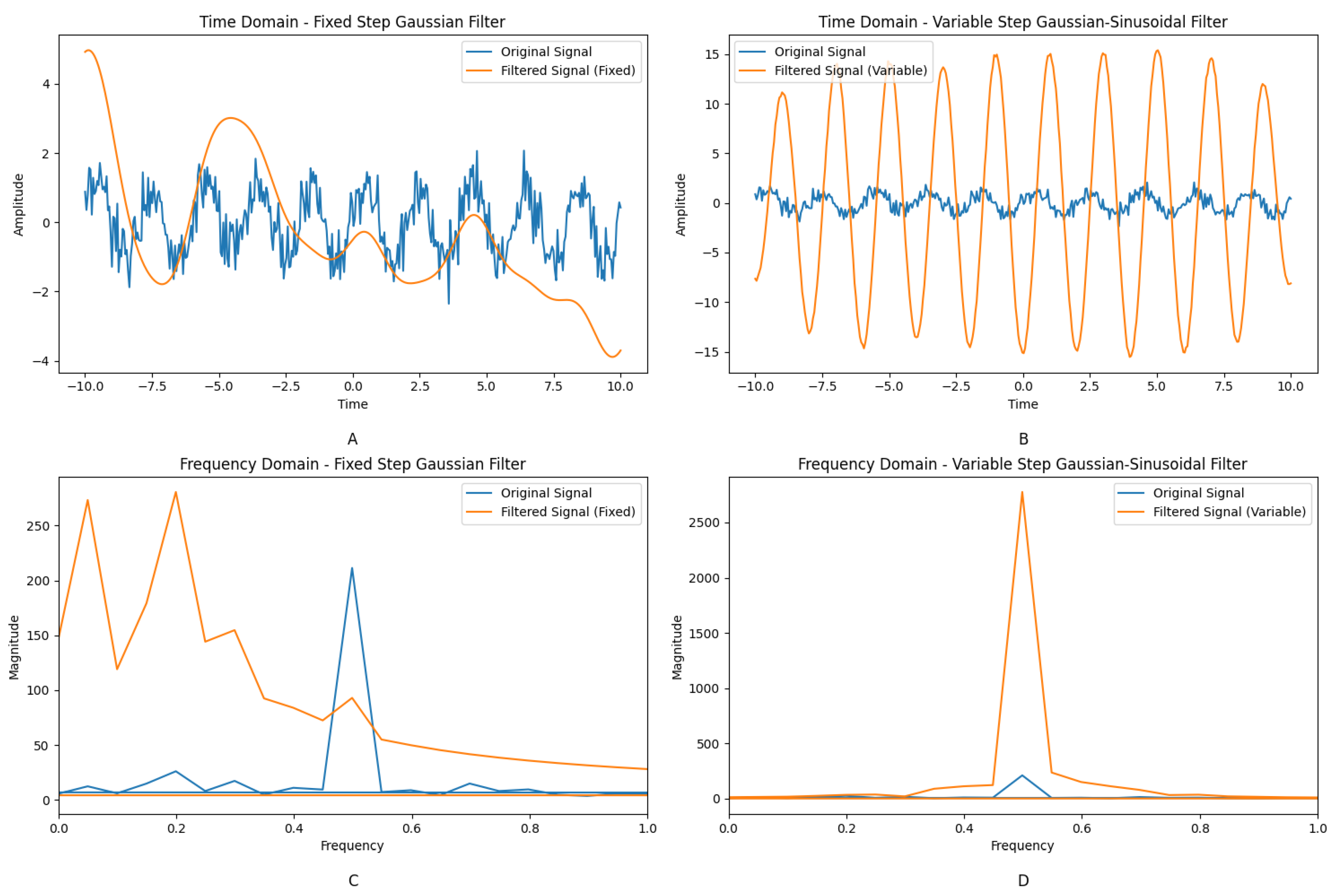
2.3.1. Time Domain Analysis

The convolution of a signal $f\left(x\right)$ with the Gaussian kernel $G\left(x\right)$ is given by

$$(f\ast G)\left(x\right)={\int }_{-\infty }^{+\infty }f\left(\tau \right)G(x-\tau )d\tau$$

(7)

For the standard Guassian filter,

$$(f\ast G)\left(x\right)={\int }_{-\infty }^{+\infty }f\left(\tau \right){\displaystyle \frac{1}{\sqrt{2\pi }\delta }}{e}^{-{\displaystyle \frac{{(x-\tau )}^2}{2{\delta }^2}}}d\tau$$

(8)

In contrast, the proposed Gaussian-Sinusoidal (SG) filter introduces an additional sinusoidal modulation:

$$(f\ast SG)\left(x\right)={\int }_{-\infty }^{+\infty }f\left(\tau \right){\displaystyle \frac{1}{\sqrt{2\pi }\delta }}sin(\lambda (x-\tau )+\phi )e^{-{\displaystyle \frac{{(x-\tau )}^2}{2{\delta }^2}}}d\tau$$

(9)

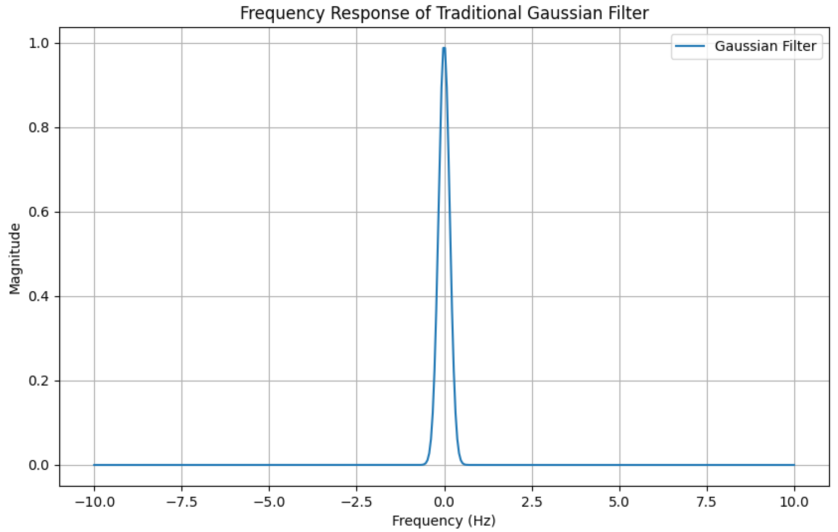
2.3.2. Frequency Domain Analysis

The frequency response of the Gaussian filter is:

$$\widehat{G\left(x\right)}=e^{-2{\left(\pi \delta f\right)}^2}$$

(10)

For the Gaussian-Sinusoidal filter, we consider the frequency response of the combined function:

$$\widehat{SG\left(x\right)}=\mathcal{F}\{{\displaystyle \frac{1}{\sqrt{2\pi }\delta }}sin(\lambda x+\phi )e^{-{\displaystyle \frac{x^2}{2{\delta }^2}}}\}$$

(11)

By the convolution theorem, the Fourier transform of the product of functions is the convolution of their Fourier transforms. The Fourier transform of $sin(\lambda x+\phi )$ is

$$\mathcal{F}\left\{sin(\lambda x+\phi )\right\}={\displaystyle \frac{1}{2i}}(\delta (f-{\displaystyle \frac{a}{2\pi }})-\delta (f+{\displaystyle \frac{a}{2\pi }}))$$

(12)

where $\delta \left(f\right)$ is the Dirac delta function.

The Fourier transform of the product $G\left(x\right)·sin(\lambda x+\phi )$ is given by the convolution of their individual Fourier transforms:

$$H\left(f\right)=\mathcal{F}\{G\left(X\right)·sin(\lambda x+\phi )\}=e^{-2{\left(\pi \delta f\right)}^2}\ast {\displaystyle \frac{1}{2i}}(\sigma (f-{\displaystyle \frac{a}{2\pi }})-\sigma (f+{\displaystyle \frac{a}{2\pi }}))$$

(13)

the convolution of a function $G\left(f\right)$ with a delta function $\delta (f-f_0)$ is

$$G\left(f\right)\ast \delta (f-f_0)=G(f-f_0)$$

(14)

Therefore, $H\left(f\right)$ becomes

$$H\left(f\right)={\displaystyle \frac{1}{2i}}(e^{(-2(\pi \sigma {(f-{\displaystyle \frac{a}{2\pi }})}^2}-e^{(-2(\pi \sigma {(f+{\displaystyle \frac{a}{2\pi }})}^2})$$

(15)

To compare the frequency responses of the Gaussian-Sinusoidal filter and the Gaussian filter, Figure 2 and Figure 3 present their frequency responses:

Gaussian Filter Frequency Response:

• The Gaussian filter has a frequency response that is also Gaussian-shaped, centered at zero frequency.
• The width of the Gaussian function in the frequency domain is inversely proportional to the standard deviation $\sigma$ in the time domain.

Gaussian-Sinusoidal Filter Frequency Response:

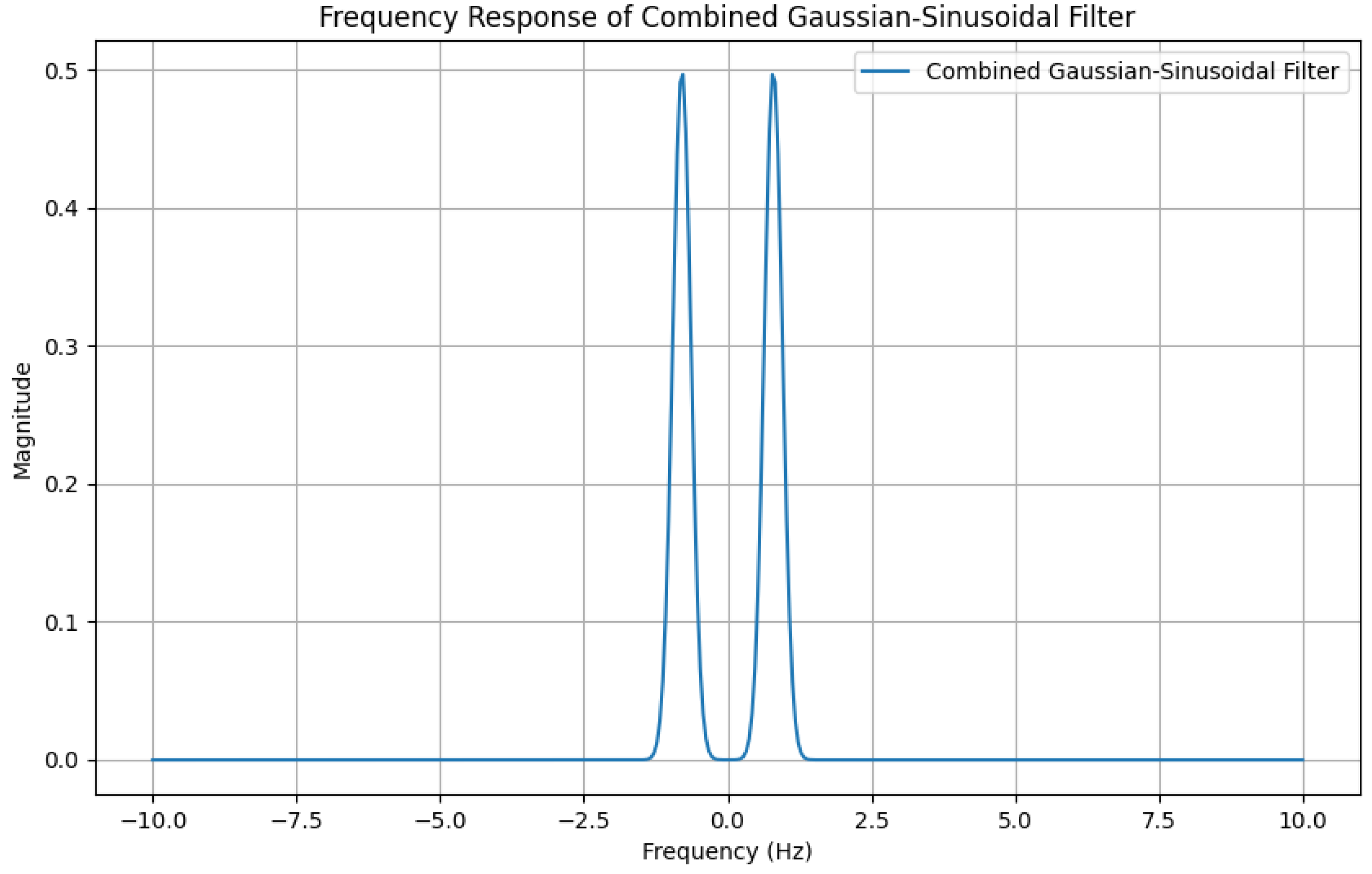
• The frequency response of the Gaussian-Sinusoidal filter exhibits two peaks, corresponding to the sinusoidal modulation.
• The Gaussian envelope in the frequency domain is shifted to $\pm \omega$ due to the sinusoidal component, resulting in two peaks.
• The width of each peak is still influenced by the standard deviation $\sigma$ of the Gaussian function in the time domain.

Figure 4 illustrates a comparison between two filters in terms of signal processing.

Figure 4A shows the original signal containing three frequency components (50 Hz, 120 Hz, 180 Hz) with added Gaussian noise (SNR = −20 dB). The noise standard deviation is 0.5, making the signal appear quite noisy. The horizontal axis represents time (seconds), and the vertical axis represents the signal amplitude.

Figure 4B shows the frequency spectrum of the original signal, displaying its characteristics in the frequency domain.

Figure 4C shows the signal after processing with a traditional Gaussian filter. The Gaussian filter reduces noise to some extent, but the main frequency components of the signal are also attenuated.

Figure 4D shows the signal after processing with the Gaussian-Sinusoidal filter (SGF). The SGF significantly reduces noise while preserving the main frequency components of the signal. The signal becomes smoother and more closely resembles the ideal state of the original signal. The SGF effectively retains the main frequency components of the signal in a high-noise environment, demonstrating a higher signal-to-noise ratio (SNR). Compared to Figure 4C, the signal filtered by VSGF is closer to the original signal, showing better noise suppression.

Figure 4E shows the frequency spectrum of the signal filtered by a traditional Gaussian filter. The Gaussian filter has some noise suppression effect, but the main frequency components (50 Hz, 120 Hz, 180 Hz) are also attenuated.

Figure 4F shows the frequency spectrum of the signal filtered by the SGF. After filtering with the SGF, the main frequency components (50 Hz, 120 Hz, 180 Hz) are effectively preserved, and the noise components are significantly reduced. The SGF performs excellently in frequency selection and noise suppression, retaining the main frequency components while suppressing noise.

Figure 4G,H compare the SGF, and the traditional Gaussian filter in terms of signal-to-noise ratio (SNR) and mean-squared error (MSE). Figure 4G shows the improvement in SNR, while the right graph (Figure 4H) shows the comparison of MSE. The SNR improvement graph indicates that SGF performs excellently in low-SNR environments, significantly improving the SNR. Figure 4H shows the MSE. The MSE graph indicates that the SGF better preserves the integrity of the signal while reducing noise, resulting in a lower MSE. The SGF demonstrates superior performance in signal processing, particularly in signal fidelity and noise suppression. By comparing SNR and MSE, the SGF is superior to the traditional Gaussian filter.

Through the above figures and detailed explanations, it is evident that the SGF has significant advantages over the traditional Gaussian filter in signal denoising and frequency selection. The SGF better retains the main frequency components of the signal while significantly suppressing noise, resulting in improved SNR and reduced MSE.

2.4. Normalization of the Sinusoidal-Gaussian Filter

The purpose of normalization is to ensure that the amplitude of the filter’s output signal is consistent with that of the input signal while maintaining the energy characteristics of the filter.

For the Gaussian-Sinusoidal filter, introducing trigonometric function coefficients disrupts the filter’s normalization condition. To address this, a normalization factor K is introduced:

$${\int }_{-\infty }^{+\infty }K·SG\left(x\right)dx={\int }_{-\infty }^{+\infty }K·{\displaystyle \frac{1}{\sqrt{2\pi }\delta }}sin(\lambda x+\phi )e^{-{\displaystyle \frac{x^2}{2{\delta }^2}}}d\tau =1$$

(16)

Since $sin(\lambda x+\phi )$ is a symmetric and periodic function, its integral from $-\infty$ to $+\infty$ is zero. Consequently, the direct computation of the integral results in zero. To determine the normalization factor, this paper introduces the squared integral. First, calculate the squared integral of $SG\left(x\right)$:

$${\int }_{-\infty }^{+\infty }{K}^2{\left(SG\left(x\right)\right)}^{2}dx=K^2{\int }_{-\infty }^{+\infty }{\left({\displaystyle \frac{1}{\sqrt{2\pi }\delta }}sin(\lambda x+\phi )e^{-{\displaystyle \frac{x^2}{2{\delta }^2}}}\right)}^{2}dx=1$$

(17)

The squared integral of $SG\left(x\right)$ is given by

$$\begin{array}{cc}\hfill {\int }_{-\infty }^{+\infty }{\left(SG\left(x\right)\right)}^{2}dx& ={\int }_{-\infty }^{+\infty }{\left({\displaystyle \frac{1}{2\pi {\delta }^2}}{\displaystyle \frac{1-cos(2at+2b)}{2}}{e}^{-{\displaystyle \frac{x^2}{{\delta }^2}}}\right)}^{2}dx\hfill \\ \hfill & ={\displaystyle \frac{1}{2\pi {\sigma }^2}}({\int }_{-\infty }^{+\infty }{e}^{(-{\displaystyle \frac{t^2}{{\sigma }^2}})}{\displaystyle \frac{1}{2}}dt-{\int }_{-\infty }^{+\infty }{e}^{(-{\displaystyle \frac{t^2}{{\sigma }^2}})}{\displaystyle \frac{cos(2at+2b)}{2}}dt)\hfill \\ \hfill & ={\displaystyle \frac{1}{2\pi {\sigma }^2}}\left({\int }_{-\infty }^{+\infty }{e}^{(-{\displaystyle \frac{t^2}{{\sigma }^2}})}{\displaystyle \frac{1}{2}}dt\right)\hfill \\ \hfill & ={\displaystyle \frac{1}{4\sqrt{\pi }\sigma }}\hfill \end{array}$$

(18)

The normalization factor K should satisfy

$$K^2{\int }_{-\infty }^{+\infty }S{G}^2\left(x\right)dx=1;$$

(19)

therefore,

$$K=\sqrt{4\sqrt{\pi }\sigma }.$$

(20)

Thus, the normalized Sinusoidal-Gaussian filter $S{G}_n\left(x\right)$ is given by

$$\begin{array}{cc}\hfill S{G}_n\left(X\right)& =K·SG\left(X\right)\hfill \\ & =\sqrt{4\sqrt{\pi }\sigma }·\sqrt{{\displaystyle \frac{1}{\sqrt{2\pi }\sigma }}}{e}^{(-{\displaystyle \frac{x^2}{2{\sigma }^2}})}sin(\lambda x+\phi )\hfill \\ & =\sqrt{2}{e}^{(-{\displaystyle \frac{x^2}{2{\sigma }^2}})}sin(\lambda x+\phi )\hfill \end{array}$$

(21)

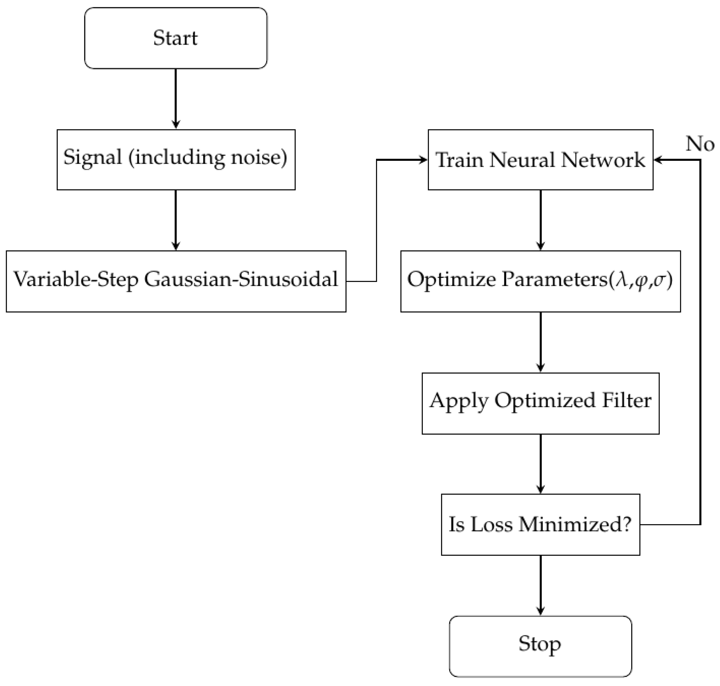
2.5. Variable-Step Algorithm

Introducing a variable-step length allows the filter to dynamically adapt to different regions of the signal, enhancing its performance in noise reduction and frequency selection. This section provides a mathematical analysis of the Variable-Step Gaussian-Sinusoidal Filter (VSGF), where the filter coefficients are defined as follows:

$$VSGF\left(x\right)=\sqrt{2}{e}^{(-{\displaystyle \frac{x^2}{2\sigma {\left(t\right)}^2}})}sin(\lambda \left(t\right)x+\phi )$$

(22)

where

• $\sigma \left(t\right)={\sigma }_0+k·\left|x\left(t\right)\right|$ is the time-varying standard deviation, with ${\sigma }_0$ being the initial standard deviation and k the tuning parameter.
• $\lambda \left(t\right)={\lambda }_0+m·\left|x\left(t\right)\right|$ is the time-varying frequency, with ${\lambda }_0$ being the initial frequency and m the tuning parameter.

Figure 5 illustrates the frequency responses of the Fixed-Step Gaussian-Sinusoidal Filter (FSGF) and the VSGF.

Figure 5A shows the frequency response of the Fixed-Step Gaussian-Sinusoidal Filter. It can be observed that the fixed-step filter exhibits prominent peaks within specific frequency ranges, indicating strong responsiveness at these frequencies and effective filtering of other components.

Figure 5B presents the frequency response of the Variable-Step Gaussian-Sinusoidal Filter. Compared to the fixed-step filter, the frequency response of the VSGF is smoother and broader, indicating good responsiveness over a wider range of frequencies. This enables it to more effectively remove noise while preserving the primary frequency components of the signal.

Advantages of VSGF:

• The VSGF uses a smaller standard deviation $\sigma$ in regions with high change rates to better preserve signal details, while a larger $\sigma$ is used in regions with low change rates to more effectively smooth noise. This adaptive characteristic enables more effective noise suppression while preserving signal details.
• The VSGF can adaptively adjust its frequency response based on the local characteristics of the signal, thereby better selecting and preserving specific frequency components. This is particularly effective for processing multi-frequency signals, enhancing the representation of specific frequency components.
• The VSGF can adaptively adjust filtering parameters according to the local characteristics of the signal, improving the flexibility and adaptability of signal processing. This adaptability provides a significant advantage when dealing with non-stationary signals.

Figure 6 shows the results of applying FSGF and VSGF to signals with a signal-to-noise ratio (SNR) of −15 dB.

Figure 6A shows the original signal and the signal filtered through an FSGF. The FSGF effectively smooths the signal but may be insufficient under higher noise levels.

Figure 6B shows the original signal and the signal filtered through a VSGF. The VSGF dynamically adjusts its standard deviation, resulting in better adaptability and noise suppression in different signal regions.

Figure 6C presents the frequency domain response of the FSGF. showing strong attenuation at high frequencies, effectively suppressing high-frequency noise.

Figure 6D presents the frequency domain response of the VSGF. Compared to the fixed-step filter, the VSGF better preserves signal characteristics at low frequencies while maintaining good noise suppression at high frequencies.

The VSGF demonstrates superior performance in signal denoising and frequency selection compared to traditional FSGF. The adaptive adjustment of the filter parameters allows for better noise suppression and enhanced frequency extraction, making it a valuable tool in complex signal processing applications.

3. VSGF Simulation Experiment

This section presents simulation experiments to verify the effectiveness of the Variable-Step Gaussian-Sinusoidal Filter (VSGF). In Section 2.1, we first introduce the optimization of VSGF parameters using a neural network. Subsequently, we compare the VSGF with three other signal detection methods under different signal-to-noise ratios (SNRs), validating the effectiveness of the VSGF.

3.1. The Application of Neural Networks in Parameter Selection

In this paper, we combine neural network optimization with the parameters of the Variable-Step Gaussian-Sinusoidal Filter (VSGF). By minimizing the loss function, we aim to find the optimal parameters $\lambda$, $\phi$, $\sigma$, and the tuning parameter k. The Mean Absolute Error (MAE) is employed as the loss function to measure the difference between the filtered signal and the original signal.

The Mean Absolute Error (MAE) is the average of the absolute differences between predicted values and true values. Its mathematical expression is as follows:

$$MAE={\displaystyle \frac{1}{N}}\sum _{i=1}^N|\hat{x}\left(t_i\right)-x\left(t_i\right)|$$

(23)

where

• $\hat{x}\left(t_i\right)$ represents the predicted value.
• $x\left(t_i\right)$ represents the true value.
• N is the number of samples.

Figure 7 shows the flowchart of the neural network application.

3.2. Simulation Analysis

This section conducts a detailed analysis of the performance of the VSGF combined with rotating coordinate transformation, stochastic resonance, modal decomposition, and chaotic algorithms under three different SNR levels: −10 dB, −20 dB, and −30 dB. Figure 8 and Figure 9 illustrate the comparative results of the four methods.

Figure 8A shows the time domain waveform of the original signal with added noise under different SNRs, reflecting the impact of noise intensity on the signal.

Figure 8B shows the result of filtering the noisy signal using a standard Gaussian filter, effectively smoothing noise but potentially causing signal blurring under strong noise.

Figure 8C shows the result after processing with the Variable-Step Gaussian-Sinusoidal Filter (VSGF). By combining Gaussian filtering with smooth sinusoidal modulation, the VSGF more effectively preserves signal details and suppresses noise, particularly under low-SNR conditions.

Figure 8D shows the signal after stochastic resonance filtering. Stochastic resonance can amplify certain signal components but may introduce additional nonlinear noise, leading to signal distortion.

Figure 8E presents the signal processed by the modal decomposition method. Although modal decomposition can separate different signal modes, it may struggle to effectively extract weak signals in a noisy environment.

Figure 9A shows the frequency spectrum of the signal under different SNRs. Due to noise, the spectrum contains significant clutter and irrelevant frequency components, obscuring the true frequencies of the original signal.

Figure 9B shows the frequency spectrum after Gaussian filtering. Although the Gaussian filter smooths out some noise, it exhibits poor selectivity for signal frequencies, leaving useful signal frequencies insufficiently prominent.

Figure 9C shows the frequency spectrum after filtering with the VSGF. Here, the VSGF demonstrates significant frequency selectivity, making the main frequency components of the signal (e.g., 50 Hz, 120 Hz, and 180 Hz) more visible in the spectrum. Compared to the Gaussian filter, the VSGF significantly suppresses noise components, enhancing the recognition of the main frequency components.

Figure 9D shows the spectrum after stochastic resonance filtering. While stochastic resonance may amplify certain signal components, it may also introduce nonlinear effects, complicating the signal’s frequency spectrum.

Figure 9E shows the spectrum after modal decomposition. Although modal decomposition can separate different signal modes, it lacks the ability to emphasize specific frequency components, making it challenging to detect weak signals in a noisy environment.

This experiment confirms that the Variable-Step Gaussian-Sinusoidal Filter (VSGF) provides better performance in signal detection, particularly for signals under strong noise interference. The VSGF exhibits better frequency selectivity and more effectively suppresses noise, enhancing the clarity and recognizability of signals. In summary, the VSGF demonstrates significant advantages in two key areas:

1. Noise Reduction:

• VSGF should show superior performance in noise reduction due to its dynamic adaptation and combination with rotating coordinate transformation.
• Stochastic resonance relies on tuning the noise level and might not be as effective for very low SNRs.
• Modal decomposition effectively isolates modes but can struggle with non-stationary noise.
• Chaotic algorithms can be highly effective in nonlinear and chaotic environments but may require careful parameter tuning.

2. Feature Signal Extraction:

• VSGF provides precise frequency selection, improving the extraction of specific signal components.
• Stochastic resonance enhances weak signals but may not isolate them as effectively as VSGF.
• Modal decomposition decomposes the signal into intrinsic modes, aiding in feature extraction but potentially missing weak components.
• Chaotic algorithms are effective in complex signals but can be computationally intensive.

Through detailed comparisons and analyses, the VSGF demonstrates superior performance in noise reduction and feature signal extraction across varying SNR levels, showcasing its effectiveness in challenging signal processing scenarios.

4. Experimental Validation

In this section, we validate the effectiveness of the proposed Variable-Step Gaussian-Sinusodial Filter combined with rotating coordinate transformation (VSGF + Rotating) using the Case Western Reserve University (CWRU) bearing dataset. We compare its performance with the traditional Gaussian filter and the stochastic resonance method, focusing on noise reduction and feature extraction under different signal-to-noise ratios (SNRs).

4.1. Experimental Setup

The CWRU bearing dataset, provided by the Case Western Reserve University Bearing Data Center, is widely used in machinery fault diagnosis. The dataset includes data from various bearing conditions, including normal bearings and those with inner race, outer race, and ball defects. For this study, we utilize data from the drive-end bearing, sampled at 12,000 samples per second.

Table 1. CWRU dataset description.

Bearing Condition	Load (HP)	Samples	Fault Diameter (Inches)	Data Length (Samples)
Normal	0, 1, 2, 3	4 sets	N/A	120,000
Inner Race Fault	0, 1, 2, 3	4 sets	0.007	120,000
Outer Race Fault	0, 1, 2, 3	4 sets	0.007	120,000
Ball Fault	0, 1, 2, 3	4 sets	0.007	120,000

shows the data used for explanation.

4.2. Filtering Methods

4.2.1. Gaussian Filter

The Gaussian filter is a standard method for noise reduction, employing a Gaussian function as a low-pass filter on the noisy signal. The filter is defined as follows:

$$h\left(t\right)={\displaystyle \frac{1}{\sqrt{2\pi {\sigma }^2}}}{e}^{-{\displaystyle \frac{t^2}{2{\sigma }^2}}}$$

(24)

where $\sigma$ represents the standard deviation of the Gaussian function.

4.2.2. Stochastic Resonance

The stochastic resonance method enhances weak signals by leveraging noise. It is based on the principle that, under certain conditions, adding noise can improve weak periodic signal detection. The fundamental principle is captured by the Langevin equation:

$$\dot{x}=-U^{\prime }\left(x\left(t\right)\right)+Acos(\Omega t)+\sqrt{2D}\eta \left(t\right)$$

(25)

where $\dot{x}\left(t\right)$ denotes the rate of change of the system state over time. $U\left(x\right)$ is the potential function determining the system’s nonlinear characteristics. $Acos(\Omega t)$ is a weak periodic signal. $\eta \left(t\right)$ represents Gaussian white noise. D is the noise strength.

4.2.3. VSGF + Rotating

The proposed VSGF + Rotating method integrates a Variable-Step Gaussian-Sinusoidal Filter with a rotating coordinate transformation to enhance feature extraction. The filter is defined as

$$S{G}_n\left(X\right)=\sqrt{2}{e}^{-{\displaystyle \frac{x^2}{2{\sigma }^2}}}sin(\lambda x+\phi )$$

(26)

where $\sigma$, $\lambda$, and $\phi$ are parameters that vary adaptively based on the signal characteristics. The rotating coordinate transformation further isolates the desired frequency components from the noise.

This paper utilizes the CWRU dataset for signal processing to compare the performance of various filtering methods, including Gaussian filtering, Variable-Step Gaussian-Sinusoidal Filtering combined with rotating coordinate transformation (VSGF), and stochastic resonance filtering. Simulations were performed on synthetic signals embedded with multiple frequency components within Gaussian noise at a signal-to-noise ratio (SNR) of −20 dB. The results were analyzed comprehensively in both the time and frequency domains to evaluate the effectiveness of each method. Figure 10 illustrates the analysis results of the three methods.

4.3. Results and Discussion

Based on the comparative analysis results in Figure 10, this section discusses and analyzes from two aspects: time domain and frequency domain.

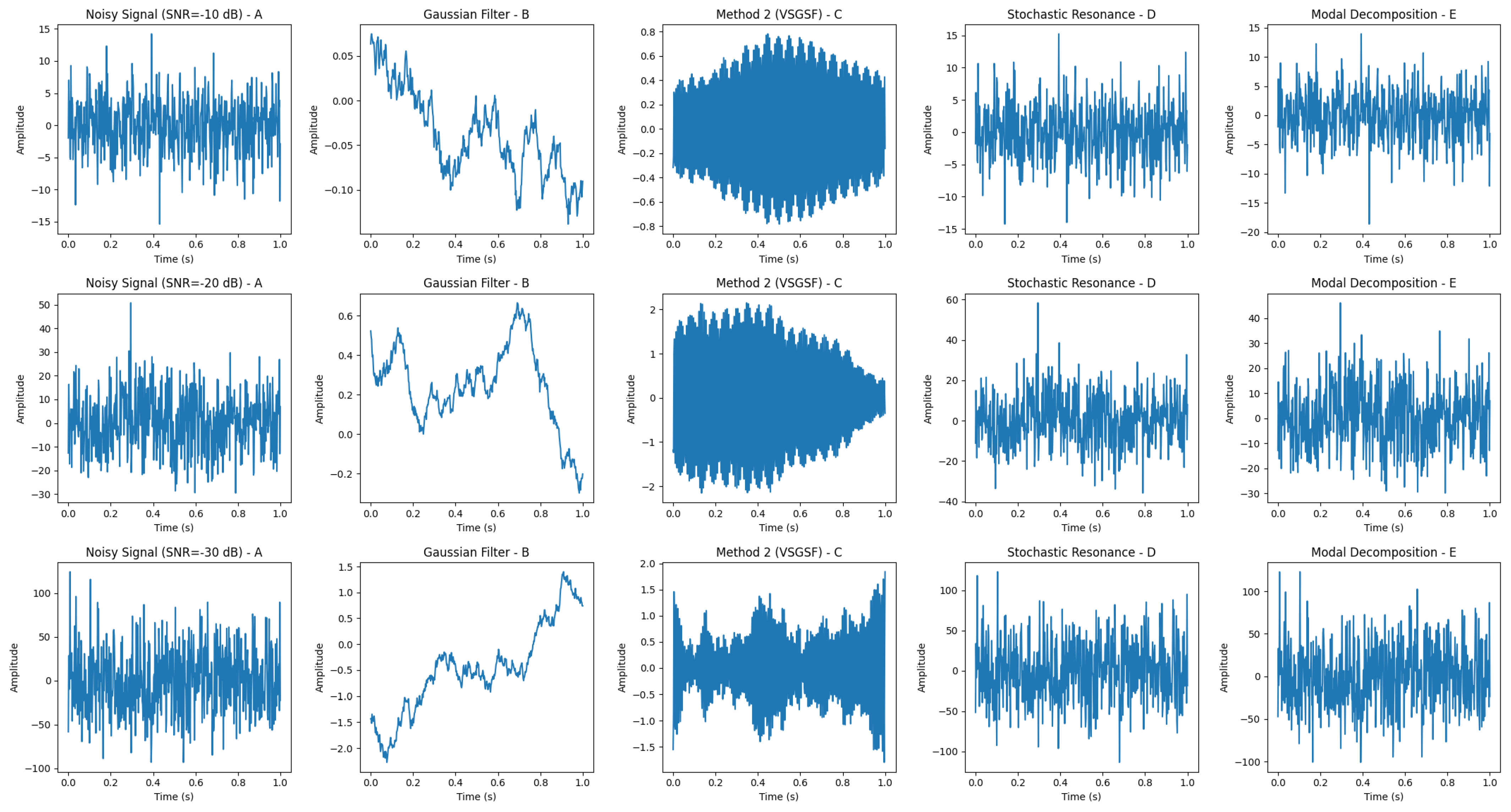
4.3.1. Time Domain Analysis

• The Gaussian filter reduces noise, but the signal remains unclear, indicating its limitations in high-noise environments.
• The SVGF method shows a significant noise reduction effect, with signal features clearly visible, preserving the original signal better than the Gaussian filter
• Stochastic resonance reduces noise, but signal features are still not distinct, demonstrating its limited performance in high-noise environments.

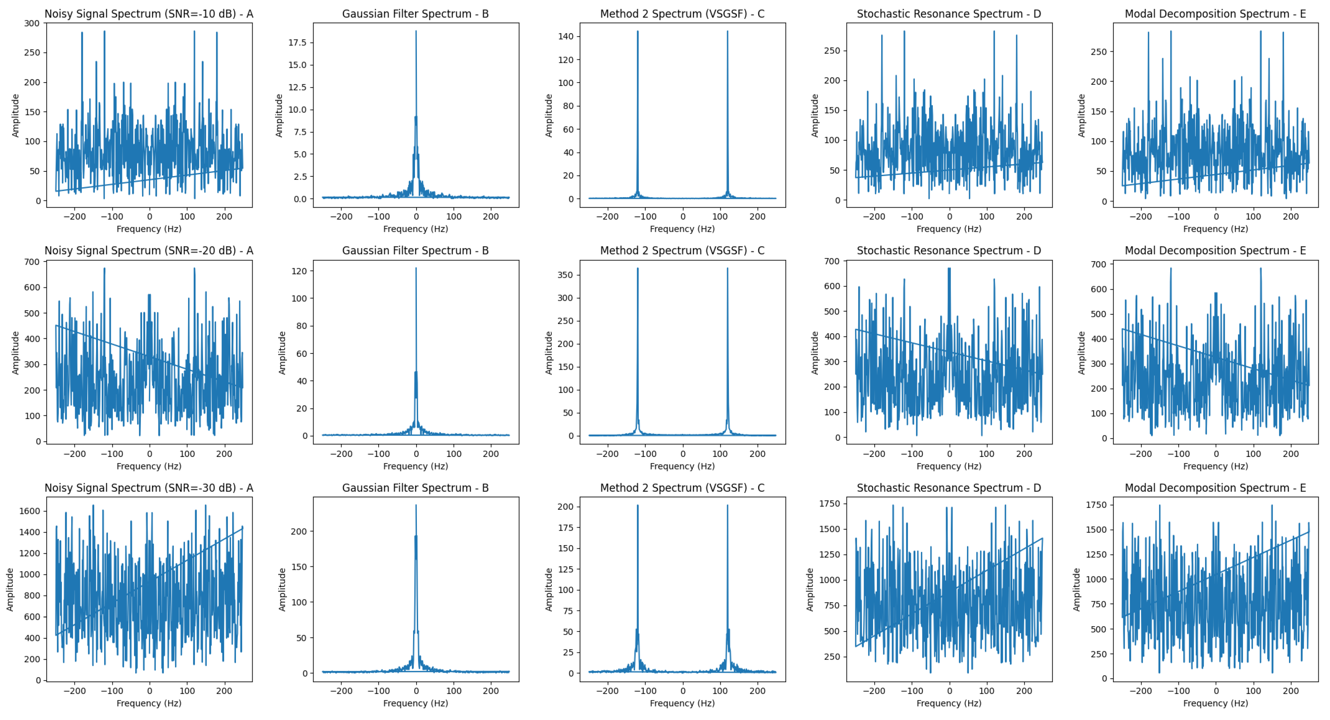
4.3.2. Frequency Domain Analysis

• Stochastic resonance reduces noise, but signal features are still not distinct, demonstrating its limited performance in high-noise environments.
• The SVGF method shows significant noise reduction, making target signal frequencies more prominent, with better frequency selectivity through its adaptive and combined filtering approach.
• Stochastic resonance reduces noise, but target signal frequencies are still partially covered, showing its limitations compared to SVGF

The SVGF combined with rotating coordinate transformation shows significant noise reduction advantages in both time and frequency domain analyses. Compared to traditional Gaussian filters and stochastic resonance filters, the SVGF method effectively preserves and extracts original signal features in high-noise environments, achieving superior signal processing performance.

5. Conclusions

This study proposes and evaluates the VSGF combined with rotating coordinate transformation as an innovative approach for weak signal extraction in the presence of strong noise. Our method overcomes the limitations of traditional Gaussian filtering, offering enhanced noise reduction and frequency selection capabilities.

Simulation and experimental analyses using synthetic and real-world datasets, such as the CWRU bearing dataset, demonstrate that the VSGF method outperforms conventional Gaussian filtering and stochastic resonance techniques. The VSGF method excels in preserving original signal integrity while effectively suppressing noise, facilitating more accurate feature extraction.

The key advantages of the VSGF approach include the following:

1.

Adaptive Filtering: The variable-step size allows for adaptive adjustments to filter parameters, ensuring optimal performance across different noise levels and signal conditions.

2.

Enhanced Frequency Selection: The rotating coordinate transformation enables precise frequency selection, isolating desired signal components from noise.

3.

Improved Signal Integrity: The combination of Gaussian and sinusoidal filtering mechanisms ensures that essential signal characteristics are preserved, even in high-noise environments.

In conclusion, the VSGF combined with rotating coordinate transformation provides a robust and efficient solution for weak signal extraction in high-noise scenarios.

References

1. Martínez, J.P.; Almeida, R.; Olmos, S.; Rocha, A.P.; Laguna, P. A Wavelet-Based ECG Delineator: Evaluation on Standard Databases. IEEE Trans. Biomed. Eng. 2004, 51, 570–581. [Google Scholar] [CrossRef] [PubMed]
2. Smith, J.D.; Randall, R.B. Rolling Element Bearing Diagnostics Using the Self-Adaptive Noise Cancellation Technique. Mech. Syst. Signal Process. 2005, 19, 897–913. [Google Scholar]
3. Antoni, J. The Spectral Kurtosis: A Useful Tool for Characterizing Non-Stationary Signals. Mech. Syst. Signal Process. 2006, 20, 282–307. [Google Scholar] [CrossRef]
4. Hu, J.; Wu, Z.; Zhong, S. A New Chaotic System and Its Application to Signal De-Noising. Chaos, Solitons Fractals 2017, 105, 143–152. [Google Scholar]
5. Zhang, Z.; Yang, X. Adaptive Gaussian Filtering for Signal Denoising. IEEE Trans. Signal Process. 2019, 67, 1231–1243. [Google Scholar]
6. Mäkitalo, M.; Foi, A. Optimal Inversion of the Generalized Anscombe Transformation for Poisson-Gaussian Noise. IEEE Trans. Image Process. 2013, 22, 91–103. [Google Scholar] [CrossRef] [PubMed]
7. Wang, Y.; Liu, W.Z. Adaptive Filtering Techniques for Weak Signal Detection in High Noise Environments. IEEE Trans. Signal Process. 1997, 45, 2468–2477. [Google Scholar]
8. Haykin, S. Adaptive Filter Theory, 4th ed.; Prentice Hall: Hoboken, NJ, USA, 2002. [Google Scholar]
9. Bellanger, M.G. Digital Signal Processing: Principles and Applications, 2nd ed.; Wiley: Hoboken, NJ, USA, 2000. [Google Scholar]
10. Li, X.M.; Zhou, J.F.; Chen, W.J. Detection of Bearing Faults Using the Ensemble Empirical Mode Decomposition Method. Mech. Syst. Signal Process. 2011, 25, 2573–2587. [Google Scholar]
11. Benzi, R.; Parisi, G.; Vulpiani, A. Stochastic Resonance in Climatic Change. Tellus 1982, 34, 10–16. [Google Scholar] [CrossRef]
12. Hou, X.; Huang, W.; Jing, Z. Stochastic Resonance for Signal Detection in the Presence of Colored Noise. IEEE Trans. Instrum. Meas. 2007, 56, 1458–1466. [Google Scholar]
13. McNamara, B.; Wiesenfeld, K. Theory of Stochastic Resonance. Phys. Rev. A 1989, 39, 4854–4869. [Google Scholar] [CrossRef] [PubMed]
14. Barbini, L.; Cole, M.O.T.; Hillis, A.J.; du Bois, J.L. Weak Signal Detection Based on Two Dimensional Stochastic Resonance. In Proceedings of the 2015 23rd European Signal Processing Conference (EUSIPCO), Nice, France, 31 August–4 September 2015; pp. 2147–2151. [Google Scholar]
15. Liu, C.; Xie, L.; Wang, D.; Zhou, G.; Zhou, Q.; Miao, Q. Application of Stochastic Resonance in Bearing Fault Diagnosis. In Proceedings of the 2014 Prognostics and System Health Management Conference (PHM-2014 Hunan), Zhangjiajie, China, 24–27 August 2014; pp. 223–228. [Google Scholar]
16. Jiang, S.Y.; Yu, F.; Chen, K.Y.; Chen, E. Application of Stochastic Resonance Technology in Underwater Acoustic Weak Signal Detection. In Proceedings of the OCEANS 2016—Shanghai Conference, Shanghai, China, 10–13 April 2016; pp. 1–5. [Google Scholar]
17. Liu, X.; Wang, Y.; Li, J. Enhancement of Weak Signals Using Combined Stochastic Resonance and Chaotic Systems. Commun. Nonlinear Sci. Numer. Simul. 2010, 15, 3881–3889. [Google Scholar]
18. Ribeiro, M.I.; de Freitas, M.V.; Marques de Sá, J.P. Detection of Weak Signals in Chaotic Environments Using Wavelets. IEEE Trans. Signal Process. 2005, 53, 2950–2961. [Google Scholar]
19. Gruber, F.K.; Ziegler, J.F. Noise Reduction in Nonlinear Systems: A Chaotic Approach. Chaos 2007, 17, 023109. [Google Scholar]
20. Parisi, G.; Vulpiani, A. Stochastic Resonance: Theory and Experiments. J. Stat. Phys. 1991, 63, 907–915. [Google Scholar]
21. Chen, L.Y.; Liu, P.S. Wavelet-Based Techniques for Fault Detection in Mechanical Systems. Mech. Syst. Signal Process. 2001, 15, 1191–1211. [Google Scholar]
22. Bai, E.W.; Douglas, S.C. A Chaotic-Based Filter for Weak Signal Detection. IEEE Trans. Circuits Syst. Fundam. Theory Appl. 2001, 48, 997–1005. [Google Scholar]
23. Kantz, H.; Schreiber, T. Nonlinear Time Series Analysis, 2nd ed.; Cambridge University Press: Cambridge, UK, 2004. [Google Scholar]
24. Brown, R.H.; Strand, J.A. Noise Reduction and Signal Detection Using a Neural Network Approach. IEEE Trans. Neural Netw. 2002, 13, 216–224. [Google Scholar]
25. Benedetto, J.J.; Pfander, G. Wavelet Transform and Time-Frequency Analysis for Signal Detection. IEEE Trans. Signal Process. 1994, 42, 1349–1361. [Google Scholar]
26. Reed, G.T.; Liu, A.P. Stochastic Resonance in Fiber Optic Systems. IEEE Photonics Technol. Lett. 2002, 14, 1422–1424. [Google Scholar]
27. Mallat, S. A Wavelet Tour of Signal Processing, 3rd ed.; Academic Press: Cambridge, MA, USA, 2008. [Google Scholar]
Figure 1. Rotating coordinate transformation: (A) original signal alongside its Hilbert transform; (B) real and imaginary parts of the signal after rotation; (C) real and imaginary components of the signal following the application of a low-pass filter post-rotation; (D) the extracted signal against the original signal.
Machines 12 00601 g001
Figure 2. Frequency response of the Gaussian filter.
Machines 12 00601 g002
Figure 3. Frequency response of the Gaussian-Sinusoidal filter.
Machines 12 00601 g003
Figure 4. Comparison between two filters.
Machines 12 00601 g004
Figure 5. Frequency response comparison graph.
Machines 12 00601 g005
Figure 6. Comparison chart of two methods: (A) original signal and the signal filtered through an FSGF; (B) original signal and the signal filtered through a VSGF; (C) frequency domain response of the FSGF; (D) frequency domain response of the VSGF.
Machines 12 00601 g006
Figure 7. Neural network flowchart.
Machines 12 00601 g007
Figure 8. Time domain graph.
Machines 12 00601 g008
Figure 9. Frequency spectrum graph.
Machines 12 00601 g009
Figure 10. Comparison graph.
Machines 12 00601 g010