Abstract
Computer-vision-based plant leaf segmentation technology is of great significance for plant classification, monitoring of plant growth, precision agriculture, and other scientific research. In this paper, the YOLOv8-seg model was used for the automated segmentation of individual leaves in images. In order to improve the segmentation performance, we further introduced a Ghost module and a Bidirectional Feature Pyramid Network (BiFPN) module into the standard Yolov8 model and proposed two modified versions. The Ghost module can generate several intrinsic feature maps with cheap transformation operations, and the BiFPN module can fuse multi-scale features to improve the segmentation performance of small leaves. The experiment results show that Yolov8 performs well in the leaf segmentation task, and the Ghost module and BiFPN module can further improve the performance. Our proposed approach achieves a 86.4% leaf segmentation score (best Dice) over all five test datasets of the Computer Vision Problems in Plant Phenotyping (CVPPP) Leaf Segmentation Challenge, outperforming other reported approaches.
1. Introduction
The segmentation of individual leaves of a plant is a prerequisite for measuring more complex phenotypic traits such as shape, color, area, mass, or texture, or for counting the number of leaves. For instance, biologists cultivate model plants like Arabidopsis (Arabidopsis thaliana) and tobacco (Nicotiana tabacum) in controlled environments, monitoring and documenting their phenotypes to investigate the performance of plants in general. Previously, such phenotypes were annotated manually by experts, but recently, image-based non-destructive approaches have gained attention among plant researchers in plant classification, monitoring of plant growth, precision agriculture, and other scientific research [1].
Leaf segmentation can be divided into two categories: one is isolated leaf segmentation and identification, and the other is live plant leaf segmentation. The second category can further be divided into two sub-categories, leaf semantic segmentation and leaf instance segmentation.
Isolated leaf segmentation and identification usually uses datasets with leaves that have been cut from plants and imaged individually. Leaf classification and disease identification are the most common tasks in this category. Françoise used a binary thresholding technique to segment the leaf and extract leaf texture to classify plants into families [2]. Shoaib used modified U-Net to segment the tomato leaf and then Inception Net to classify the segmented images by different levels of disease [3]. For this task, in most cases there is only one leaf in the image. Some leaf classification approaches can even be done without the segmentation stage. For example, Bin Wang used a parallel two-way convolutional neural network to classify the leaf category in Flavia [4], Swedish [5], and Leafsnap [6] datasets and achieved above 91% performance in all three datasets [7]. Various types of deep convolution networks were employed in leaf classification tasks such as lightweight CNN [8], Siamese network [9], and ResNet [10,11]. These works show that for isolated leaf segmentation and identification, if the images are taken carefully with only one leaf in the center and a clear background, researchers can achieve very good performance in their tasks even if they omit the segmentation or detection stage.
Live plant leaf segmentation is another category and has many differences from isolated leaf segmentation because live plant leaf segmentation is to segment the leaves of the plant in the image, while isolated leaf segmentation is to segment the leaves that have been cut from the plant and placed on a plain background. The typical difficulties of live plant leaf segmentation include: (1) The live plant usually has multiple leaves. (2) The leaves are shot from different angles, so they have different shapes, poses, and appearances. (3) The background may not be very clear. (4) It is hard to find clearly discernible boundaries among overlapping leaves. Thus, live plant leaf segmentation usually requires more complex algorithms and models to handle the complex background and lighting conditions in the image, as well as to handle the deformation and overlapping of leaves.
Live plant leaf segmentation involves two different tasks, leaf semantic segmentation and leaf instance segmentation. The difference between semantic segmentation and instance segmentation lies in the objects they segment. Semantic segmentation classifies each pixel into a category (such as leaves or background), while instance segmentation divides each object into a separate entity (such as a single leaf).
Leaf semantic segmentation is usually required by precision agriculture, agricultural robotics, and weed identification. Andres Milioto presented a CNN-based semantic segmentation approach for crop fields, separating sugar beet plants, weeds, and background based on RGB data in real-time [12]. Tanmay Anand proposed a deep learning framework, AgriSegNet, for automatic detection of farmland anomalies using multiscale attention semantic segmentation of UAV-acquired images [13]. Sovi Guillaume Sodjinou used U-Net and K-means subtractive algorithm to apply the semantic segmentation of crops and weeds [14].
Many studies leverage leaf instance segmentation, including growth monitoring and regulation, and counting [15,16]. In one study, Bhugra et al. proposed a framework that relies on a graph-based formulation to extract leaf shape knowledge for the task of leaf instance segmentation [17]. Numerous creative approaches employ varied types of mathematics, modeling and computer science approaches including 3D data augmentation [18], generative adversarial networks, and Mask R-CNN [19].
In this work, we put our focus on the problem of leaf instance segmentation and proposed two improved versions of the YOLOv8-seg model for automatic segmentation of individual leaves in images. To enhance the segmentation performance, we introduce a Ghost module and a BiFPN module to the standard YOLOv8 model. The Ghost module can generate multiple intrinsic feature maps through several inexpensive transformation operations, while the BiFPN module can fuse multi-scale features to improve the segmentation performance of small leaves. We also confirmed through ablation experiments that the BiFPN and Ghost module do help to improve the classification effect to a certain extent.
2. Materials and Methods
2.1. Datasets
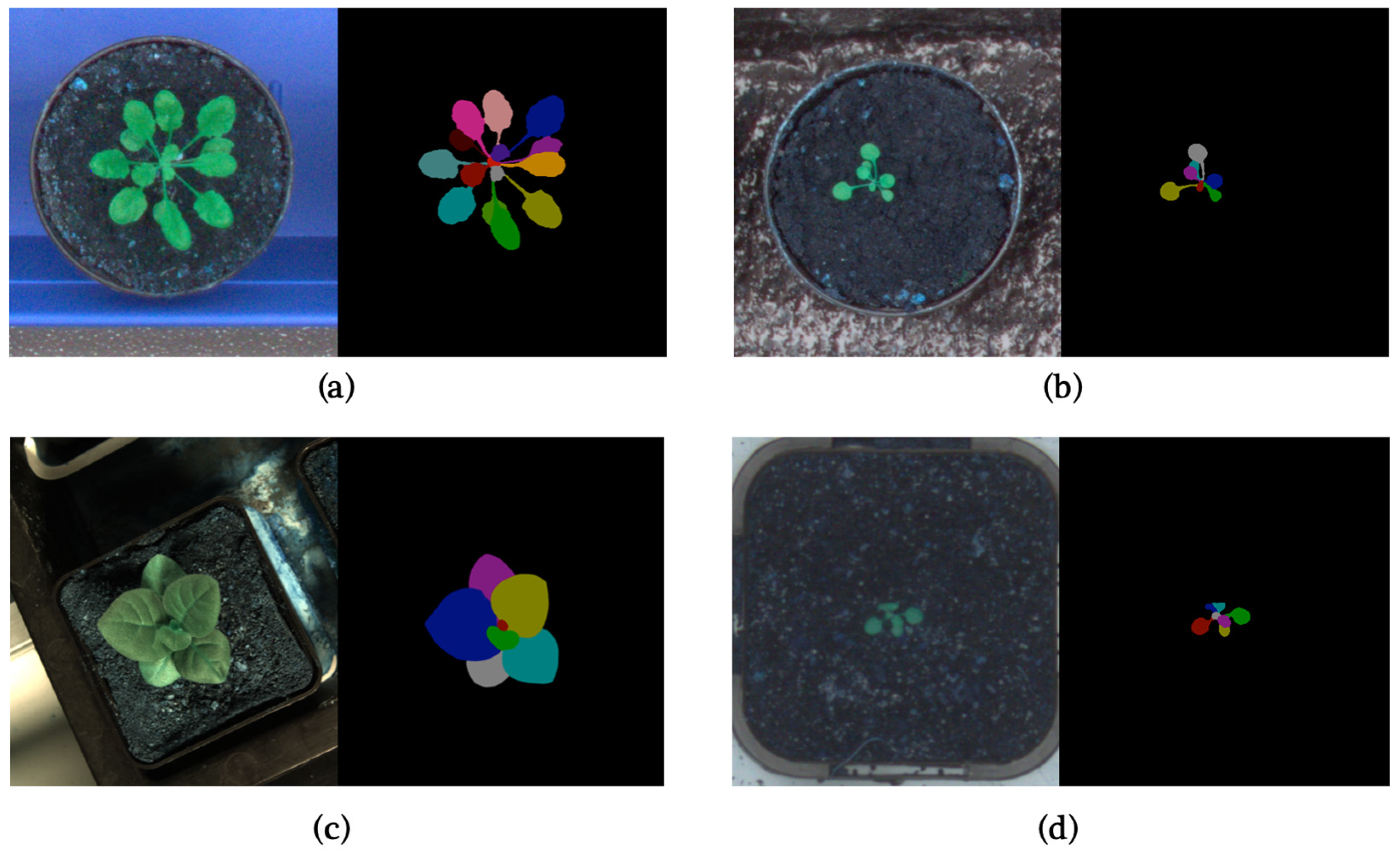
In this paper, to make the results as comparable as possible, we use the CVPPP LSC dataset [1,20,21] for training and validating our model. It is one of the most significant datasets in this field and has almost become a benchmark for these tasks. The CVPPP LSC dataset was presented in the Leaf Segmentation Challenge of Computer Vision Problems in Plant Phenotyping Workshop, which is also the origin of the name CVPPP LSC. The LSC 2014 training dataset includes three subsets (A1, A2, A3), with A1 and A2 consisting of 159 time-lapse images of Arabidopsis and A3 consisting of 27 images of tobacco. In LSC 2017, a new subset A4 was introduced, consisting of 624 images of Arabidopsis shared by Dr. Hannah Dee from Aberystwyth [21]. Figure 1 shows typical images from different datasets, and Table 1 is a brief summary of the LSC training dataset.
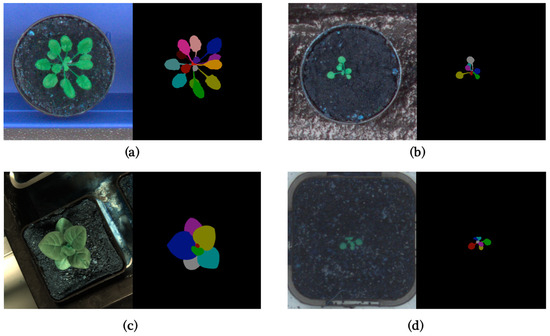
Figure 1.
(a) Typical image in A1; (b) Typical image in A2; (c) Typical image in A3; (d) Typical image in A4.

Table 1.
Summary of the LSC training dataset.
The LSC testing set can be divided into two groups. The first group is A1–A4, which corresponds to the training set of A1–A4 respectively. The second group is A5, which is basically a combination of the data of A1–A4. Table 2 is a brief summary of the LSC testing dataset. CVPPP did not release the ground truth of the testing set; to evaluate the performance of the testing set, the results need to be uploaded to the competition website (https://codalab.lisn.upsaclay.fr/competitions/8970, accessed on 1 January 2024) for online calculation, and the performance of the testing set needs to be uploaded and evaluated via the competition site.
Table 2.
Summary of the LSC testing dataset.
2.2. Framework
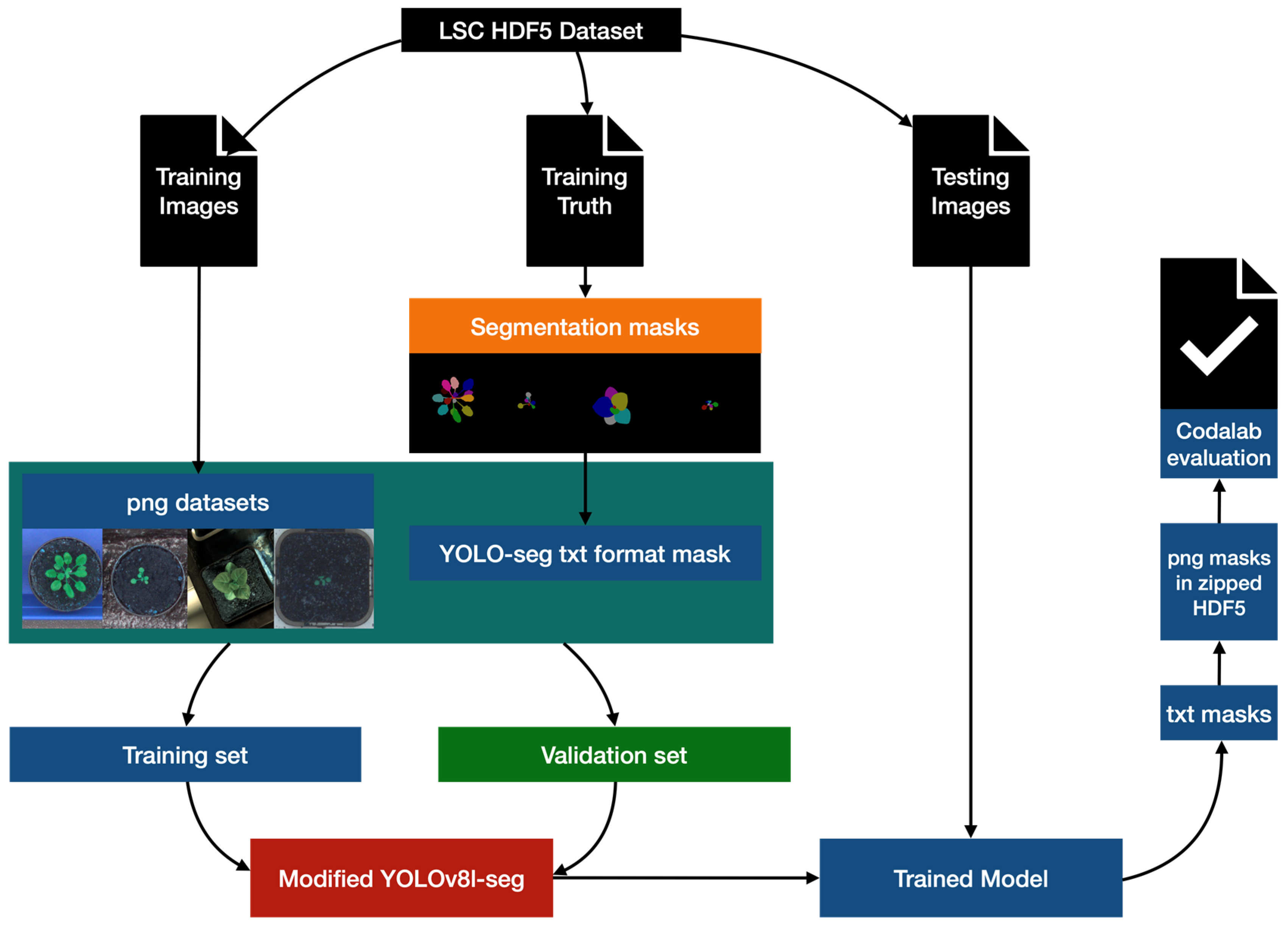
The working process of data processing, model training, and model validation is shown in Figure 2. It was not always the case that datasets were provided in a format which was compatible with YOLOv8. In the preprocessing, we employ the h5py and OpenCV to appropriately transform the dataset into png format with txt masks [22,23]. To prevent overfitting, we have created a training set that is 3/4 the size of the original training set and a validation set that is 1/4 the size by taking the fourth one after every three in the file list. Then we develop a modified YOLOv8-seg model and train the model with the split training and validation sets, and use it to segment the official test set. We incorporate the BiFPN module (Bidirectional Feature Pyramid Network) [24] and Ghost module [25] into the original YOLOv8-seg model to enhance the segmentation performance. The segmentation results were submitted to the competition website for performance evaluation.

Figure 2.
The working process of data processing, model training, and model validation.
2.3. Methods
In this work, the YOLOv8 model and two modified versions were used for leaf segmentation. YOLO introduced a new, simplified way to perform simultaneous object detection and classification in images [26,27]. The latest version of YOLO is Yolov8, released in January 2023 by Ultralytics [28], who also created the earlier version YOLOv5 [29]. YOLOv8 uses techniques similar to YOLOACT [30] to provide support for instance segmentation.
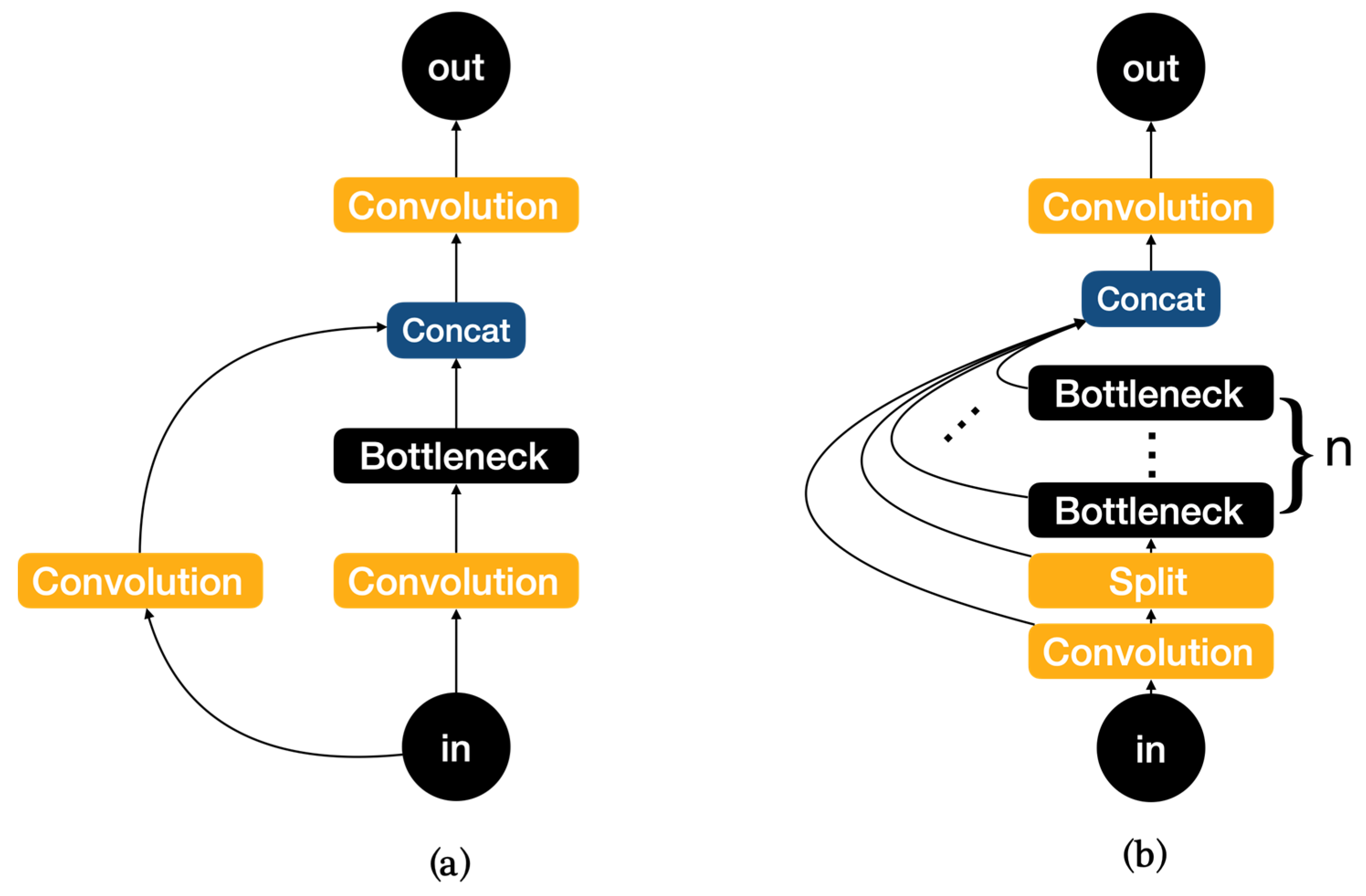
The network structure mainly consists of backbone, neck, and head, with YOLOv8 replacing the C3 module of YOLOv5 with the C2f module in the backbone as shown in Figure 3. It is easy to see that the C2f module has a richer gradient flow. The head section adopts a popular decoupled head structure which separates the classification and detection heads, and also is converted from anchor-based to anchor-free, reducing the number of box predictions and speeding up the non-maximum impression (NMS). In loss calculation, Task Aligned Assigner is used for positive sample allocation and Distribution Focal Loss is introduced. The data augmentation section incorporates the operation of closing Mosaic enhancement in the last 10 epochs of YOLOX [31], which can effectively improve accuracy.
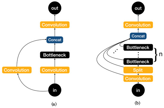
Figure 3.
(a)Architecture of C3. (b) Architecture of C2f.
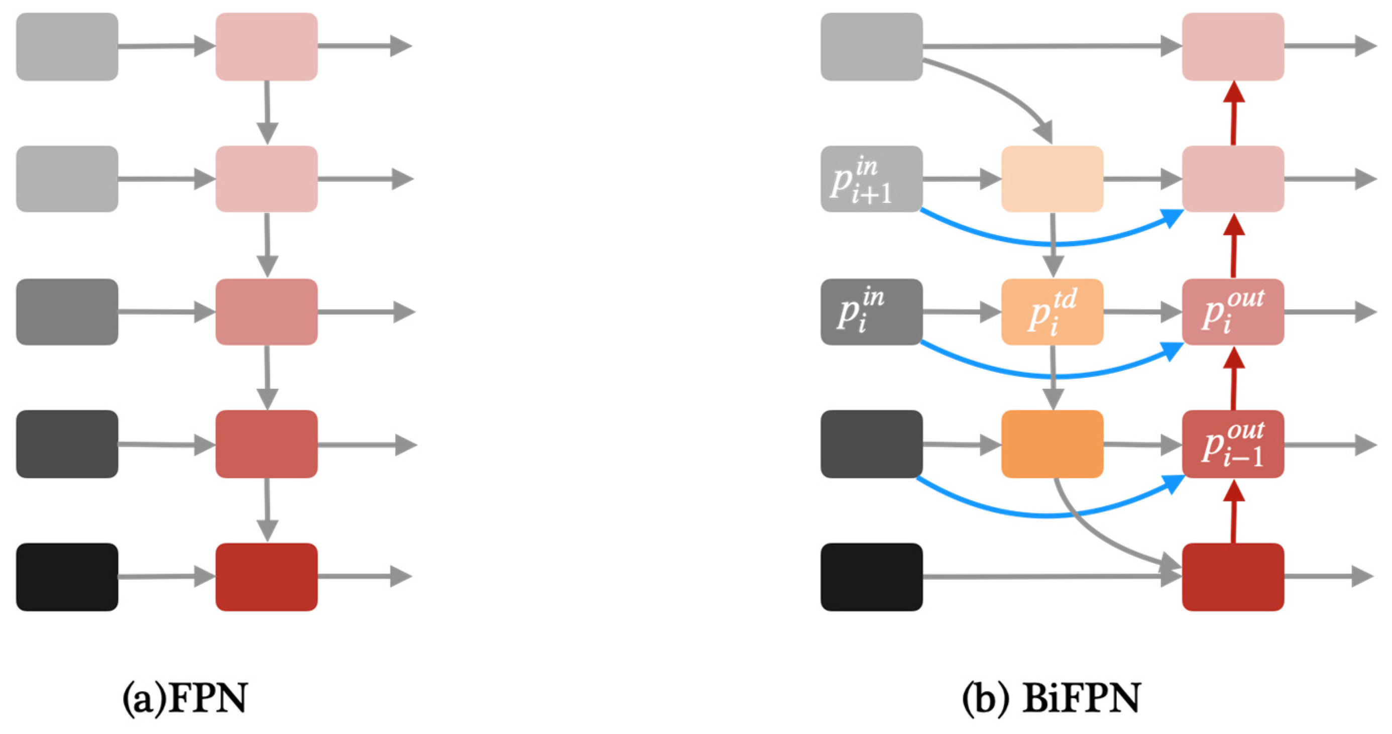
Apart from YOLOv8, we proposed two modified YOLOv8 models in this paper, one of which is YOLOv8-BiFPN. FPN (Feature Pyramid Network) is used to solve the problem of multi-scale in object detection, which can improve detection performance with small targets [32]. Compared with the traditional FPN network, BiFPN adds skip connections between the input and output features in the same layer [24]. Due to using the same scale, adding skip connections can better extract and transfer feature information. Figure 4 shows the architecture of FPN and BiFPN.

Figure 4.
(a)Architecture of FPN. (b) Architecture of BiFPN.
BiFPN uses weighted feature fusion to fuse input feature maps of different resolutions. The weights in BiFPN were calculated as follows:
where , represent the intermediate transition feature of the i-th layer on the top-down pathway and the last output feature of the i-th layer on the bottom-up pathway. , are the weight parameters of the input of the current layer and the input of the next layer. In Formula (2), , , respectively represent weight of the current layer input, the weight of the transition unit output in the current layer, and the weight of the previous layer output. ϵ is a hyperparameter to prevent the gradient from vanishing [24].
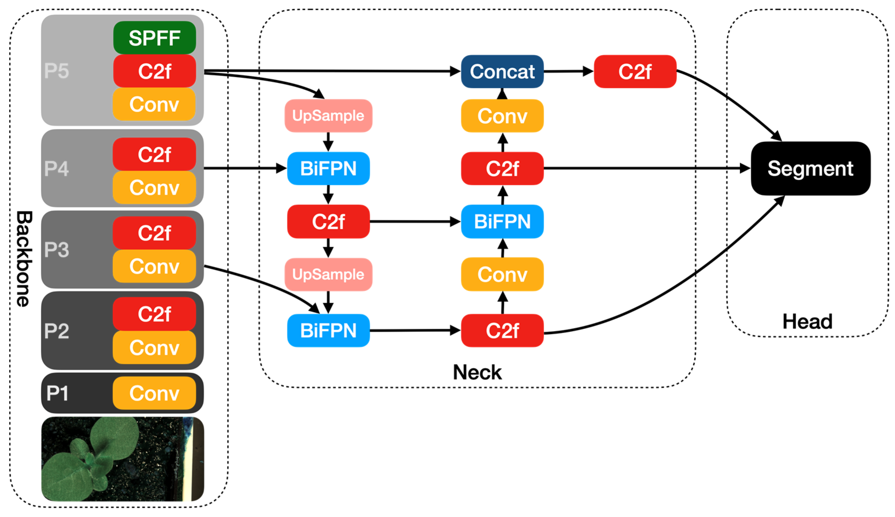
In this paper, we incorporate the BiFPN module into the neck of the YOLOv8 module and present the YOLOv8-BiFPN model. Figure 5 shows the architecture of the YOLOv8-BiFPN model.

Figure 5.
The YOLOv8-BiFPN network architecture diagram.
The other modified YOLOv8 model that we propose in this article is YOLOv8-Ghost. The Ghost module splits the original convolutional layer into two parts and utilizes fewer filters to generate several intrinsic feature maps. Then, a certain number of cheap transformation operations will be further applied for generating Ghost feature maps efficiently [25]. Figure 6 shows the principle of the Ghost module. The Ghost module includes two sets of feature maps: the intrinsic feature, which is composed of the convolution of the input, and another set which is composed of some cheap transformation results of the first set (in this work the cheap transformation refers to the 5 × 5 convolution). Thus, the Ghost module can reduce the computational effort and generate richer feature maps, which is helpful in enhancing the generalizing ability of the model. We incorporate the Ghost module into the backbone of the YOLOv8 model and present the YOLOv8-Ghost model. Figure 7 presents the YOLOv8-Ghost network architecture. It consists of backbone, neck, and head; the backbone is a Feature Pyramid Network [32] to deal with the multi-scale issue and the neck is a Path Aggregation Network [33] to boost the information flow. From Figure 7, one can find that the convolution block in P4 of the backbone was substituted with the Ghost module to boost the generalizing ability.
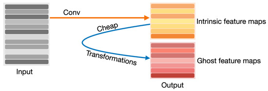
Figure 6.
Principle of Ghost module.
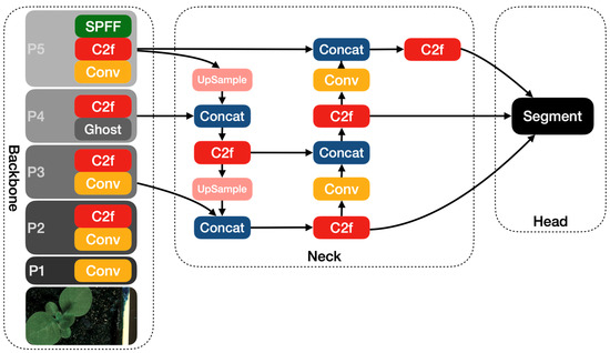
Figure 7.
The YOLOv8-Ghost network architecture diagram.
2.4. Data Augmentation
Data augmentation is a technique commonly used in machine learning to increase the size and diversity of a dataset. It involves applying various transformations to the existing data to create new, synthetic samples. In this paper, we apply some data augmentations supported by YOLOv8, including adjustment of the HSV color, translating the image horizontally and vertically by a fraction, scaling the image by a gain factor to simulate objects at different distances, flipping the image upside down and left to right with the specified probability, rotating the image randomly within the specified degree range, combining four training images into one to simulate different scene compositions, and randomly erasing a portion of the image during classification training. The specific parameters for data augmentation are shown in Table 3.
Table 3.
Data augmentation parameters.
2.5. Software and Hardware Environments
The experiments were conducted on a computer with Nvidia Tesla P100 GPU. The detailed information of software and hardware environments are listed in Table 4.
Table 4.
Summary of software and hardware environments.
3. Results
3.1. Evaluation Metrics
To evaluate the performance of multi-object segmentation, the five metrics used in the CVPPP Leaf Segmentation Challenge were adopted for result comparison [34], i.e., the Best Dice () [35,36], Symmetric Best Dice (), Foreground–Background Dice (), Difference in Count (), and Absolute Difference in Count ().
Dice is a metric in binary segmentation that measures the degree of overlap between the ground truth and the algorithmic result , as defined in Equation (3).
Best Dice is defined as:
Symmetric Best Dice is the symmetric average Dice among all leaves, which is defined as:
Foreground–Background Dice () is the Dice score of the foreground mask (i.e., masks of all leaves).
Difference in Count () is a metric used to evaluate how well an algorithm identifies the correct number of leaves present, and is defined as:
Absolute Difference in Count () is the absolute difference in object count.
3.2. Segmentation Results
The leaf instance segmentation on the CVPPP LSC dataset was performed by the YOLOv8-seg and the two modified versions, namely the YOLOv8-BiFPN and YOLOv8-Ghost. Taking into comprehensive consideration the data size, the GPU memory size, and the performance, we chose the l-scale in the scale selection of the three models. During the training stage, all of the training sets (A1, A2, A3, A4) were combined together to create a larger dataset; 3/4 was used for training, and 1/4 was used for validation. Since the original size of the dataset is close to 512 × 512, all of the images were resized to 512 × 512. The neural network was trained through 250 epochs with batch size 16. Figure 8 shows selected examples of test images from the four datasets. From each dataset we chose two examples: one to show the effectiveness of the methods and one to show limitations. We have four datasets, so eight pictures were selected and composed into the eight rows in Figure 8. The first column is the test leaf image, the second column is the segmentation result using YOLOv8, the third column is the segmentation result using YOLOv8-BiFPN, and the fourth column is the segmentation result using YOLOv8-Ghost. We show visually the segmentation outcomes for each method together and overlay the numbers of the evaluation measures on the images (Best Dice in the top left corner, Difference in Count in the top right, Symmetric Best Dice in the bottom left, and Foreground–Background Dice in the bottom right).
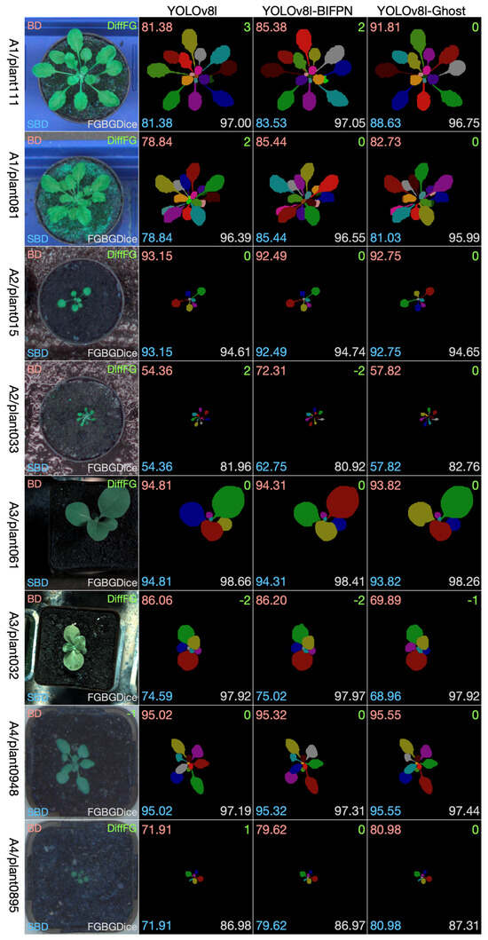
Figure 8.
Selected results on test images from each dataset.
For these eight test data examples, we see that all of the three methods perform well in the segmentation task. There is not a certain method that is absolutely better than the other two methods. It can be observed that YOLOv8-Ghost is more precise in the counting of the number of leaves, but in other indicators, the three methods have their own advantages and disadvantages.
The segmentation result for the whole test dataset is shown in Table 5. It can be seen that among the three methods, the performance of the two modified versions is slightly better than that of the original YOLOv8. The performance of YOLOv8-BiFPN is slightly better in and , while the performance of YOLOv8-Ghost is slightly better in , , , and than that of the other two methods.
Table 5.
Segmentation and counting results on the testing dataset.
We also compared our results with other reported works, as shown in Table 6. Because the results for test sets A5 and A6 were not reported in their papers, only the results for test sets A1, A2, and A3 were compared. From Table 6, one can see that the proposed YOLOv8-BiFPN and YOLOv8-Ghost outperform other approaches with respect to many indicators.
Table 6.
Segmentation and counting results compared with other published methods.
In order to compare with the algorithms of other contestants, we submitted the segmentation results of YOLOv8-Ghost to the competition’s leaderboard, as it has demonstrated stronger performance on Best Dice than YOLOv8-BiFPN, and the competition website mainly uses Best Dice to determine the ranking. Our algorithm’s average ranking on the leaderboard (https://codalab.lisn.upsaclay.fr/competitions/8970#results, accessed on 20 April 2024) is third place as of writing this manuscript (20 April 2024) (our name is “pw” on the leaderboard), and the specific rankings of different test sets by different metrics are shown in Table 7.
Table 7.
Results and rankings on the leaderboard (on 20 April 2024).
4. Discussion
In the experiment, we found that the YOLOv8-based [28] methods outperform other approaches in the leaf segmentation task. Moreover, we present two modified versions, i.e., the YOLOv8-BiFPN and YOLOv8-Ghost, which can further improve the performance.
We believe that the BiFPN module [24] can add skip connections between the input and output features in the same layer, which result in better extract and transfer feature information. The Ghost module [25] can reduce the computational effort and generate richer feature maps, which is helpful in enhancing the generalizing ability of the model. Readers may think that the combination of the BiFPN and Ghost modules might further improve the performance; in fact, we conducted the corresponding experiments, but unfortunately, the results were not ideal. Only a few indicators were improved, and most of the indicators were not as positively affected as using one kind of improvement alone. This may be because the BiFPN module tends to increase the complexity on the basis of YOLOv8, while the Ghost module tends to reduce the computational complexity. In the process of combination of the BiFPN and Ghost module, the two modules may mutually influence each other, and the result is not ideal.
It can be found that there is a large number of defocused blurs in the dataset. Some corrections can be made for these defocused blurs in the pre-processing in future work. In addition, although the focus of this article is the instance segmentation of the leaves of living plants, these plants were all planted in flower pots. The leaf segmentation of plants in the fields undoubtedly is more challenging, and it is also a direction worthy of further research.
5. Conclusions
In this paper, we presented and evaluated a framework for leaf instance segmentation. The YOLOv8 model was employed for the leaf instance segmentation task; moreover, we proposed two modified versions by incorporating the BiFPN module and Ghost module into the original YOLOv8 model to enhance the leaf segmentation performance. In the experiment, we found that the three methods outperform other approaches in the leaf segmentation task, and the proposed YOLOv8-BiFPN and YOLOv8-Ghost can further improve the performance. YOLOv8-BiFPN shows better performance in FGBGDice, which is used to separate the leaf from the background, and YOLOv8-Ghost shows better performance in BestDice and leaf counting metrics like DiffFG and AbsDiffFG.
Author Contributions
P.W., P.Z. and J.B. designed the experiments. P.W., H.D., J.G., S.J. and D.M. performed the experiments. P.W. and H.D. wrote the manuscript. P.W., P.Z. and H.D. revised and edited the manuscript. All authors have read and agreed to the published version of the manuscript.
Funding
This research was funded by Northeast Agricultural University, grant number 18QC63. This research was funded by Heilongjiang Province Mathematical Society, grant numbers HSJG202202003 and HSJG202202004.
Institutional Review Board Statement
Not applicable.
Informed Consent Statement
Not applicable.
Data Availability Statement
The data presented in this study are available in GitHub repository: https://github.com/rexlagrange/cvppp_leaf_seg, accessed on 1 June 2024. These data were derived from the following resources available in the public domain: https://codalab.lisn.upsaclay.fr/competitions/8970, accessed on 1 January 2024.
Conflicts of Interest
The authors declare no conflicts of interest.
References
- Scharr, H.; Minervini, M.; French, A.P.; Klukas, C.; Kramer, D.M.; Liu, X.; Luengo, I.; Pape, J.-M.; Polder, G.; Vukadinovic, D.; et al. Leaf segmentation in plant phenotyping: A collation study. Mach. Vis. Appl. 2016, 27, 585–606. [Google Scholar] [CrossRef]
- Tery, Z.F.; Goore, B.T.; Bagui, K.O.; Tiebre, M.S. Classification of Plants into Families Based on Leaf Texture. Int. J. Comput. Sci. Netw. Secur. 2021, 21, 205–211. [Google Scholar] [CrossRef]
- Shoaib, M.; Hussain, T.; Shah, B.; Ullah, I.; Shah, S.M.; Ali, F.; Park, S.H. Deep learning-based segmentation and classification of leaf images for detection of tomato plant disease. Front. Plant Sci. 2022, 13, 1031748. [Google Scholar] [CrossRef] [PubMed]
- Wu, S.G.; Bao, F.S.; Xu, E.Y.; Wang, Y.-X.; Chang, Y.-F.; Xiang, Q.-L. A leaf recognition algorithm for plant classification using probabilistic neural network. In Proceedings of the 2007 IEEE International Symposium on Signal Processing and Information Technology, Giza, Egypt, 5–18 December 2007; pp. 11–16. [Google Scholar] [CrossRef]
- Söderkvist, O. Computer Vision Classification of Leaves from Swedish Trees. Master’s Thesis, Linkoping University, Linköping, Sweden, 2001. Available online: https://www.cvl.isy.liu.se/en/research/datasets/swedish-leaf/ (accessed on 1 January 2024).
- Kumar, N.; Belhumeur, P.N.; Biswas, A.; Jacobs, D.W.; João, V.B. Leafsnap: A Computer Vision System for Automatic Plant Species Identification. In Computer Vision—ECCV 2012, Proceedings of the 12th European Conference on Computer Vision, Florence, Italy, October 7–13, 2012; Proceedings, Part I; Fitz-gibbon, A., Lazebnik, S., Perona, P., Sato, Y., Schmid, C., Eds.; Springer: Berlin/Heidelberg, Germany, 2012; Volume 7573, pp. 502–516. [Google Scholar]
- Wang, B.; Wang, D. Plant leaves classification: A few-shot learning method based on siamese network. IEEE Access 2019, 7, 151754–151763. [Google Scholar] [CrossRef]
- Hang, Y.; Meng, X.Y.; Wu, Q.F. Application of Improved Lightweight Network and Choquet Fuzzy Ensemble Technology for Soybean Disease Identification. IEEE Access 2024, 12, 25146–25163. [Google Scholar] [CrossRef]
- Pan, J.C.; Wang, T.Y.; Wu, Q.F. Ricenet: A two stage machine learning method for rice disease identification. Biosyst. Eng. 2023, 225, 25–40. [Google Scholar] [CrossRef]
- Chen, Y.P.; Wu, Q.F. Grape leaf disease identification with sparse data via generative adversarial networks and convolutional neural networks. Precis. Agric. 2023, 24, 235–253. [Google Scholar] [CrossRef]
- Chen, Y.P.; Pan, J.C.; Wu, Q.F. Apple leaf disease identification via improved cyclegan and convolutional neural network. Soft Comput. 2023, 27, 9773–9786. [Google Scholar] [CrossRef]
- Milioto, A.; Lottes, P.; Stachniss, C. Real-time Semantic Segmentation of Crop and Weed for Precision Agriculture Robots Leveraging Background Knowledge in CNNs. In Proceedings of the 2018 IEEE International Conference on Robotics and Automation (ICRA), Brisbane, Australia, 21–25 May 2018; pp. 2229–2235. [Google Scholar] [CrossRef]
- Anand, T.; Sinha, S.; Mandal, M.; Chamola, V.; Yu, F.R. Agrisegnet: Deep aerial semantic segmentation framework for iot-assisted precision agriculture. IEEE Sens. J. 2021, 21, 17581–17590. [Google Scholar] [CrossRef]
- Sodjinou, S.G.; Mohammadi, V.; Mahama, A.T.S.; Gouton, P. A deep semantic segmentation-based algorithm to segment crops and weeds in agronomic color images. Inf. Process. Agric. 2022, 9, 355–364. [Google Scholar] [CrossRef]
- Shadrin, D.G.; Kulikov, V.; Fedorov, M.V. Instance segmentation for assessment of plant growth dynamics in artificial soilless conditions. In Proceedings of the British Machine Vision Conference(BMVC), Newcastle, UK, 3–6 September 2018. [Google Scholar]
- Yin, X.; Liu, X.M.; Chen, J.; Kramer, D.M. Multi-leaf tracking from fluorescence plant videos. In Proceedings of the 2014 IEEE International Conference on Image Processing (ICIP), Paris, France, 27–30 October 2014; pp. 408–412. [Google Scholar] [CrossRef]
- Bhugra, S.; Garg, K.; Chaudhury, S.; Lall, B. A Hierarchical Framework for Leaf Instance Segmentation: Application to Plant Phenotyping. In Proceedings of the 2020 25th International Conference on Pattern Recognition (ICPR), Taichung, Taiwan, 18–21 July 2021. [Google Scholar]
- Ward, D.; Moghadam, P.; Hudson, N. Deep leaf segmentation using synthetic data. arXiv 2018, arXiv:1807.10931. [Google Scholar] [CrossRef]
- Zhu, Y.Z.; Aoun, M.; Krijn, M.; Vanschoren, J.; Campus, H.T. Data augmentation using conditional generative adversarial networks for leaf counting in arabidopsis plants. In Proceedings of the British Machine Vision Conference(BMVC), Newcastle, UK, 3–6 September 2018; p. 324. [Google Scholar]
- Minervini, M.; Fischbach, A.; Scharr, H.; Tsaftaris, S.A. Finely-grained annotated datasets for image-based plant phenotyping. Pattern Recognit. Lett. 2016, 81, 80–89. [Google Scholar] [CrossRef]
- Bell, J.; Dee, H.M. Aberystwyth Leaf Evaluation Dataset [Data Set]. Zenodo 2016. [Google Scholar] [CrossRef]
- Collette, A. Python and HDF5; O’Reilly: Springfield, MI, USA, 2013. [Google Scholar]
- Bradski, G. The OpenCV Library. Dr. Dobb’s J. Softw. Tools 2000, 120, 122–125. [Google Scholar]
- Tan, M.X.; Pang, R.M.; Le, Q.V. EfficientDet: Scalable and efficient object detection. In Proceedings of the 2020 IEEE/CVF Conference on Computer Vision and Pattern Recognition (CVPR), Seattle, WA, USA, 13–19 June 2020; pp. 10778–10787. [Google Scholar] [CrossRef]
- Han, K.; Wang, Y.; Tian, Q.; Guo, J.Y.; Xu, C.J.; Xu, C. Ghostnet: More features from cheap operations. In Proceedings of the 2020 IEEE/CVF Conference on Computer Vision and Pattern Recognition (CVPR), Seattle, WA, USA, 13–19 June 2020; pp. 1577–1586. [Google Scholar] [CrossRef]
- Terven, J.; Córdova-Esparza, D.-M.; Romero-González, J.-A. A Comprehensive Review of YOLO Architectures in Computer Vision: From YOLOv1 to YOLOv8 and YOLO-NAS. Mach. Learn. Knowl. Extr. 2023, 5, 1680–1716. [Google Scholar] [CrossRef]
- Redmon, J.; Divvala, S.; Girshick, R.; Farhadi, A. You Only Look Once: Unified, Real-Time Object Detection. In Proceedings of the IEEE Conference on Computer Vision and Pattern Recognition (CVPR), Las Vegas, NV, USA, 26 June–1 July 2016; pp. 779–788. [Google Scholar]
- Jocher, G.; Chaurasia, A.; Qiu, J. YOLO by Ultralytics. Available online: https://github.com/ultralytics/ultralytics (accessed on 1 January 2024).
- Jocher, G. YOLOv5 by Ultralytics. Available online: https://github.com/ultralytics/yolov5 (accessed on 1 January 2024).
- Bolya, D.; Zhou, C.; Xiao, F.; Lee, Y.J. Yolact: Real-time instance segmentation. In Proceedings of the IEEE/CVF International Conference on Computer Vision (ICCV), Seoul, Republic of Korea, 27 October–2 November 2019; pp. 9156–9165. [Google Scholar] [CrossRef]
- Ge, Z.; Liu, S.T.; Wang, F.; Li, Z.M.; Sun, J. Yolox: Exceeding yolo series in 2021. arXiv 2021, arXiv:2107.08430. [Google Scholar]
- Lin, T.-Y.; Dollár, P.; Girshick, R.; He, K.; Hariharan, B.; Belongie, S. Feature pyramid networks for object detection. In Proceedings of the IEEE Conference on Computer Vision And Pattern Recognition (CVPR), Honolulu, HI, USA, 21–26 July 2017; pp. 936–944. [Google Scholar] [CrossRef]
- Liu, S.; Qi, L.; Qin, H.; Shi, J.; Jia, J. Path Aggregation Network for Instance Segmentation. In Proceedings of the 2018, IEEE/CVF Conference on Computer Vision and Pattern Recognition (CVPR), Salt Lake City, UT, USA, 18–23 June 2018. [Google Scholar]
- Leaf Segmentation Challenge Evaluation Criteria. Available online: https://codalab.lisn.upsaclay.fr/competitions/8970#learn_the_details-evaluation (accessed on 1 January 2024).
- Sørensen, T. A method of establishing groups of equal amplitude in plant sociology based on similarity of species and its application to analyses of the vegetation on Danish commons. K. Dan. Vidensk. Selsk. 1948, 5, 1–34. [Google Scholar]
- Dice, L.R. Measures of the Amount of Ecologic Association Between Species. Ecology 1945, 26, 297–302. [Google Scholar] [CrossRef]
- Pape, J.M.; Klukas, C. 3-D histogram-based segmentation and leaf detection for rosette plants. In Computer Vision-ECCV 2014 Workshops: Zurich, Switzerland, September 6–7 and 12 2014; Proceedings, Part III; Agapito, L., Bronstein, M., Rother, C., Eds.; Springer: Cham, Switzerland, 2015; pp. 61–74. [Google Scholar]


Disclaimer/Publisher’s Note: The statements, opinions and data contained in all publications are solely those of the individual author(s) and contributor(s) and not of MDPI and/or the editor(s). MDPI and/or the editor(s) disclaim responsibility for any injury to people or property resulting from any ideas, methods, instructions or products referred to in the content. |
© 2024 by the authors. Licensee MDPI, Basel, Switzerland. This article is an open access article distributed under the terms and conditions of the Creative Commons Attribution (CC BY) license (https://creativecommons.org/licenses/by/4.0/).